A less‐biased analysis of metalloproteins reveals novel zinc coordination geometries

ABSTRACT

Zinc metalloproteins are involved in many biological processes and play crucial biochemical roles across all domains of life. Local structure around the zinc ion, especially the coordination geometry (CG), is dictated by the protein sequence and is often directly related to the function of the protein. Current methodologies in characterizing zinc metalloproteins' CG consider only previously reported CG models based mainly on nonbiological chemical context. Exceptions to these canonical CG models are either misclassified or discarded as “outliers.” Thus, we developed a less‐biased method that directly handles potential exceptions without pre‐assuming any CG model. Our study shows that numerous exceptions could actually be further classified and that new CG models are needed to characterize them. Also, these new CG models are cross‐validated by strong correlation between independent structural and functional annotation distance metrics, which is partially lost if these new CGs models are ignored. Furthermore, these new CG models exhibit functional propensities distinct from the canonical CG models. Proteins 2015; 83:1470–1487. © 2015 The Authors. Proteins: Structure, Function, and Bioinformatics Published by Wiley Periodicals, Inc.

INTRODUCTION

Since the first report of zinc's necessity for carbonic anhydrase activity in 1939,1 zinc has never failed to surprise with its versatility. Zinc ions have many different roles in proteins, including structural, where zinc holds protein folds together, as in various zinc fingers2, 3, 4; enzymatic, where zinc directly or indirectly facilitates many enzymatic reactions thanks to its Lewis acid properties5, 6; and regulatory, where zinc serves as a second messenger or signaling ion and regulates other proteins' functions.7, 8 Moreover, zinc‐utilizing enzymes span all major Enzyme Commission (EC) groups: oxidoreductases, transferases, hydrolases, lyases, isomerases, and ligases. Cellular zinc homeostasis is also crucial to life.9, 10, 11 Because zinc has essential roles across all domains of life, the number of studies published on zinc metalloproteins keeps increasing significantly, especially those using modern characterization technologies such as inductively coupled plasma mass spectrometry,12 and immobilized‐metal affinity chromatography.13

On average, approximately 10% of whole proteomes are predicted to bind at least one zinc ion.14, 15 It is anticipated that more zinc metalloproteins may exist than are currently known, with functions in sensing, transporting, and buffering of zinc ions.16 Thus, thousands of zinc metalloproteins exist in any given eukaryotic proteome, requiring bioinformatics tools and methods to gain any kind of global analysis and perspective of these zinc metalloproteins.17, 18 Traditional bioinformatics analyses of protein sequence have uncovered the ubiquity of zinc metalloproteins and many of its functional roles.14, 15 However, structural bioinformatics can provide even stronger connections between zinc metalloprotein sequence and function. Among resources for structural information, the worldwide Protein Databank (wwPDB)19 serves as the central repository of atom‐resolved biological macromolecular structures. Structural databases dedicated to metalloproteins, such as MDB,20 Mespeus,21 and MetalPDB,22 also exist in order to assess metal sites in biological macromolecules.

Zinc generally binds to proteins via coordination with electronegative atoms in the protein, such as nitrogen, oxygen, and sulfur. One of the most important structural aspects of zinc binding is its coordination geometry (CG) or the spatial arrangement of coordinating atoms around the zinc ion. In this context, the coordinating atoms are known as ligand atoms or ligands; however, the amino acid residues that contain these atoms are often referred to as “ligands” as well. A metal's CG, defined by the set of proper ligands and their spatial orientation to the metal, often has functional implications.14, 23

Zinc is also a transition metal, and binds to proteins in its +2 state, which enables a stable full 3d¹⁰ and empty 4s² and 4p⁶ orbitals. This electron configuration allows zinc to stably bind four, five, and six ligands.24 As a result, zinc ions often adopt one of three major canonical CGs (cCG): tetrahedral (Tet), trigonal bipyramidal (Tbp), and octahedral (Oct), as shown in Figure 1, where the magenta balls represent zinc, and the white balls represent ligands. Because of biological variation and missing substrates, 10 minor CGs (Fig. 1) have been reported as well.18 Studies have shown that different CGs exhibit very distinct ligand compositions and functional propensities.14, 23 Thus, exploration of zinc metalloprotein structure–function relationships requires structure‐based analyses that include adequate CG representations. Classifying ligand‐type as a property of zinc coordination and not CG per se, the two most important properties that define a CG are ligand–zinc–ligand angle (angle) and zinc–ligand bond length (bond length). Also, the CGs can be classified into three‐, four‐, five‐, and six‐ligand CG based on the number of ligands coordinating the zinc ion. For a given number of ligands, there is usually only one major CG. The ideal angles of the three canonical zinc CGs are shown in Table 1.

Figure 1.

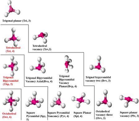
Three major (in red) and 10 minor canonical CGs of zinc metalloproteins. Magenta balls represent zinc ion, and white balls represent coordination ligands. The abbreviations and number of ligands are in parenthesis. From the lower left to the upper right, the CGs are separated by the lines with six, five, four, and three ligands, respectively.

Table 1.

Expected Angles of the Three Major Canonical CGs

Name	Total number of angles	Ideal angles and the corresponding counts
Tetrahedral (Tet)	6	109.5°—6
Trigonal bipyramidal (Tbp)	10	90°—6, 120°—3, 180°—1
Octahedral (Oct)	15	90°—12, 180°—3

CGs provide a bridge between the sequence space and functional space of metalloproteins, and therefore, knowledge about them is potentially valuable. The challenge is how to characterize a zinc's CG given its x, y, and z coordinates, which are available from structural databases such as wwPDB. The prevailing methodology is to first obtain all possible CG models of a metal from the literature, and then score a given metal site for how well it matches known CG models. The model with the highest “score” will be classified as the metal's CG. Alberts et al.25 were among the first to classify the CGs of zinc metalloproteins. They compared 111 zinc sites with ideal geometries manually, and only identified three major and one minor CG. Patel et al.26 used the deviation from the ideal CGs to classify zinc's structure. They examined 228 structures and classified them into four CGs. Liu et al.27 developed a method to identify three‐ligand and four‐ligand major CG of zinc by calculating a potential zinc center from the ligand coordinates and measuring its distance from the real zinc center. Andreini et al.18, 22 determined given PDB entries' metal CGs by first superimposing the structure to ideal CG templates, and then calculating the root‐mean‐square‐deviation value for each template.

However, in all of these studies, only known major and minor CG models are considered. Thus, if a previously unreported CG existed, specific instances of it would either be misclassified into an expected model or considered as outliers and not classified at all. In our initial analysis of CGs using only known models, we observed abnormally high variance in the angles characterizing classified groups of CG (Table 2). As we explored the factors that would cause such high variance in CG angles, we detected the existence of significant numbers of abnormally compressed angles when plotting the minimum angles of all zinc sites (Fig. 2). Normally, a minimum expected angle in any previously reported zinc CGs is 90°. However, these minimum angles center around 32° and 53°, each with a normal‐like distribution, and have not yet been investigated in any previous studies. Thus, if forcibly classified into one of the known CGs, these instances with a compressed angle will cause the high variance observed in Table 2. These initial results prompted us to develop a less‐biased method for classifying zinc CGs. Using this less‐biased analysis, we discovered previously uncharacterized zinc CGs. As far as we know, no previous study has tried to explain the high variability after classification in terms of possibly unknown CGs. Most studies simply remove “outliers” to have “acceptable” variance in their results. We have tried to directly handle and understand the reasons for high variability in zinc CG. Our efforts also include analyses of the functional annotation of these new structural classifications, which indicate distinct functional relationships for these previously uncharacterized CGs.

Table 2.

Ligand–Zinc–Ligand Angles Statistics when Forcibly Classified into Canonical CG Models [Color table can be viewed in the online issue, which is available at wileyonlinelibrary.com.]

Model	Count	Ideal angle (°)	Mean angle (°)	Standard deviation	Coefficients of variation
Tetrahedral (Tet)	10,077	109.5	109.1	8.66	0.079
Tetrahedral vacancy (Tev)	493	109.5	105.2	10.9	0.104
Trigonal bipyramidal (Tbp)	597	90	93.60	13.2	0.141
		120	116.2	13.8	0.119
		180	146.9	45.7	0.311
Trigonal bipyramidal vacancy axial (Bva)	884	90	92.56	13.9	0.150
		120	115.7	19.5	0.169
Trigonal bipyramidal vacancy planar (Bvp)	1,597	90	90.27	16.8	0.186
		120	120.8	10.7	0.089
		180	140.1	37.6	0.268
Octahedral (Oct)	325	90	89.96	6.66	0.074
		180	169.4	9.02	0.053
Square planar (Spl)	18	90	89.80	6.30	0.070
		180	168.9	5.68	0.034
Square pyramidal (Spy)	632	90a	91.84	7.23	0.079
		90p	90.97	11.0	0.121
		180	164.4	19.4	0.118
Square pyramidal vacancy (Pyv)	1,178	90a	95.02	7.86	0.083
		90p	92.71	10.1	0.109
		180	157.0	24.2	0.154
Trigonal planar (Tpl)	51	120	117.1	12.1	0.103
Overall	15,852	–	–	10.4

Figure 2.

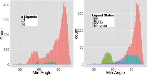
Histogram of minimum angles with respect to: (A) the number of ligands in the zinc fc‐shells and (B) ligand type for four‐ligand zinc fc‐shells. aa represents standard amino acid, nonaa represents nonstandard amino acid or any substrates from the protein, and bi represents bidentation.

METHODS

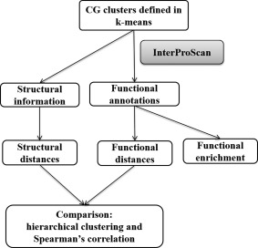
Figure 3 is an analysis flow diagram showing an overview of the analyses performed and the methods used in this work. In the end, this integrated set of analyses creates a “less‐biased” overall analysis of zinc CGs of noncluster zinc metalloproteins in the wwPDB. All analyses were completed by in‐house code written in the Perl programming language, unless noted otherwise.

Figure 3.

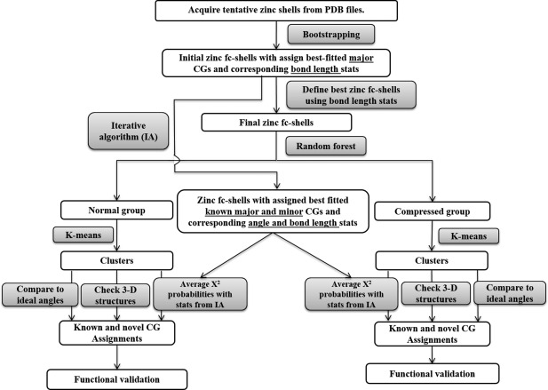
Workflow of the less‐biased analysis for novel CG detection.

Defining zinc first coordination shells

As shown in Tables 2 and 3, the angle statistics vary widely based on CG, whereas bond length statistics are rather CG agnostic and very stable (monomodal with coefficients of variation less than 0.139). Thus, we developed a less‐biased method to define zinc first coordination (fc) shells, that is, only the directly coordinating ligands, where coordinating ligands are defined primarily from bond length statistics.

Table 3.

Zinc–Ligand Bond Length Statistics when Forcibly Classified into Canonical CG Models [Color table can be viewed in the online issue, which is available at wileyonlinelibrary.com.]

Zn–X	Count	Mean bond distance (Å)	Standard deviation	Coefficients of variation
Zn‐S	26,770	2.34	0.16	0.068
Zn‐O	25,417	2.25	0.31	0.138
Zn‐N	23,582	2.14	0.18	0.084
Zn‐Cl	354	2.38	0.33	0.139
Zn‐P	182	2.97	0.12	0.040

Acquire zinc metalloproteins from PDB and create list of potential zinc ligands

We acquired structural data from the wwPDB on March 13, 2013. Our initial data filtering tools identified all PDB entries with at least one zinc atom in the HETATM record and removed entries with fewer than 20 amino acids in the SEQRES record. Next, zinc clusters were identified and removed, using two zinc atoms within 3 Å as the filter. For each remaining zinc site, we generated a list of potential zinc ligands based on non‐C/H atoms within 1.3–3.2 Å of the zinc atom.

Acquire zinc–ligand bond length statistics of major CGs (empirical bootstrapping)

For each list of potential zinc ligands, our CG evaluation tools computed the ligand–zinc–ligand angles and compared them with the ideal angles of the three major CGs, Tet, Tbp, and Oct as shown in Figure 1. Next, our tools evaluated all possible permutations of four, five, and six ligands with respect to their correspondence to each major CG. For example, if the list contained at least four potential ligands, all nonequivalent permutations of these four ligands were mapped to the ideal tetrahedral four ligands, and the corresponding angles compared with the ideal. For a potential zinc fc‐shell, our tools calculated the angle variance of a possible ligand permutation p to its corresponding CG model s (Tet, Tbp, or Oct):

$${\sigma }_p^2= \frac{1}{A}\sum _{i=1}^A{(a_i- e_{s,i})}^2, p=\mathrm{1,2},3,\dots ,\# \mathrm{p}\mathrm{o}\mathrm{s}\mathrm{s}\mathrm{i}\mathrm{b}\mathrm{l}\mathrm{e} \mathrm{p}\mathrm{e}\mathrm{r}\mathrm{m}\mathrm{u}\mathrm{t}\mathrm{a}\mathrm{t}\mathrm{i}\mathrm{o}\mathrm{n}\mathrm{s}$$ (1)

where a_i is the ith observed ligand–zinc–ligand angle, A is the total number of angles (6 for Tet, 10 for Tbp, and 15 for Oct), and e_{s , i} is the ith ideal (expected) angle of the corresponding CG model s (see Table 1 for ideal angles of different CGs). For each potential zinc fc‐shell, our tools calculated one variance for each permutation p. The permutation with the smallest variance was then identified as the initial zinc fc‐shell. The corresponding model s was assigned the given zinc as an initial best‐fitted major CG.

From all initial zinc fc‐shells identified as CG s, our tools calculated the angle statistics (mean and variance),

$${\widehat{\mu }}_{s,i}=\frac{1}{M}\sum _{j=1}^M{a}_{ij}; {\widehat{\sigma }}_{s,i}^2= \frac{1}{M-1}\sum _{j=1}^M{\left(a_{ij}- {\widehat{\mu }}_{s,i}\right)}^2 \mathrm{f}\mathrm{o}\mathrm{r} \mathrm{C}\mathrm{G} \mathrm{m}\mathrm{o}\mathrm{d}\mathrm{e}\mathrm{l} s$$ (2)

where a_ij is the observed angle i for fc‐shell j. From the identified binding ligands of all initial fc‐shells, our tools calculated element‐specific bond length statistics (mean and variance),

$${\widehat{\mu }}_t= \frac{1}{N}\sum _{j=1}^N{b}_{tj}; {\widehat{\sigma }}_t^2= \frac{1}{N-1}\sum _{j=1}^N{\left(b_{tj}-{\widehat{\mu }}_t\right)}^2 \mathrm{f}\mathrm{o}\mathrm{r} \mathrm{e}\mathrm{l}\mathrm{e}\mathrm{m}\mathrm{e}\mathrm{n}\mathrm{t} t$$ (3)

where b_tj is the jth Zn‐t bond length derived from all initial fc‐shells, and t is the given ligand element (e.g., O, N, S, …).

Define best zinc fc‐shells using bond length statistics

We then reexamined all lists of potential zinc ligands to define the final fc‐shells. All nonequivalent combinations of potential ligands were considered. We define the term χ ² probability (χ ² P‐values) as 1 minus the cumulative distribution function of a χ ² distribution. Our tools used this χ ² probability, P_q(B), as a goodness of fit measure for comparing each potential zinc fc‐shell q for any given list, where P_q(B) = 1 − P( ${\chi }^2\left(B\right) \le {\chi }_{q,\mathrm{o}\mathrm{b}\mathrm{s}}^2)$ and B is the degrees of freedom, which is the same as the number of ligands in combination q. The χ ² statistic was calculated using:

$${\chi }_{q,\mathrm{o}\mathrm{b}\mathrm{s}}^2= \sum _{j=1}^B{\left(\frac{b_{tj}- {\widehat{\mu }}_t}{{\widehat{\sigma }}_t}\right)}^2 \mathrm{f}\mathrm{o}\mathrm{r} \mathrm{p}\mathrm{o}\mathrm{t}\mathrm{e}\mathrm{n}\mathrm{t}\mathrm{i}\mathrm{a}\mathrm{l} \mathrm{c}\mathrm{o}\mathrm{m}\mathrm{b}\mathrm{i}\mathrm{n}\mathrm{a}\mathrm{t}\mathrm{i}\mathrm{o}\mathrm{n} q$$ (4)

where b_tj is the jth observed bond length with the ligand being element t, ${\widehat{\mu }}_t$, and ${\widehat{\sigma }}_t$ are the corresponding means and standard deviations of element t as calculated in bootstrapping. The ligand combination q with the highest χ ² probability P_q(B) was defined as the less‐biased best zinc fc‐shell for later clustering analyses. Although this approach identified four‐, five‐, and six‐ligand fc‐shells, we mainly explored four‐ligand zinc fc‐shells in this study, which represented the vast majority (95.7%) of the final fc‐shells identified.

Iterative algorithm for mixture canonical CG models

With the aim of both identifying the best fitting known CG based on angles and bond lengths as well as refining the parameters (means, variances of angles, and bond lengths) associated with each CG, we performed the following iterative algorithm (IA). This algorithm is in the spirit of an Expectation–Maximization algorithm. A workflow of this IA process is illustrated in Figure 4.

Figure 4.

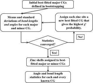
Flowchart for iterative algorithm (IA) of mixture canonical CG models.

The bootstrapping step served as the initialization step for the iteration process. It provided the initial guess of the unknown parameters ( ${\widehat{\mu }}_s, {\widehat{\sigma }}_s^2, {\widehat{\mu }}_t, \mathrm{a}\mathrm{n}\mathrm{d} {\widehat{\sigma }}_t^2)$. Mixture canonical models are the major and minor CGs in Figure 1. Our IA algorithm employed a χ ² probability, P_p(k), to determine the best fitting CG at each iteration, based on the following χ ² statistic:

$${\chi }_{p\mathrm{*}s}^2={\left(Y-{\widehat{\mu }}_{s+t}\right)}^T{C}_s^{-1}\left(Y-{\widehat{\mu }}_{s+t}\right) \mathrm{f}\mathrm{o}\mathrm{r} \mathrm{p}\mathrm{e}\mathrm{r}\mathrm{m}\mathrm{u}\mathrm{t}\mathrm{a}\mathrm{t}\mathrm{i}\mathrm{o}\mathrm{n} p \mathrm{a}\mathrm{n}\mathrm{d} \mathrm{C}\mathrm{G} \mathrm{m}\mathrm{o}\mathrm{d}\mathrm{e}\mathrm{l} s$$ (5)

where, Y is the observed angle, and bond length vector of a given zinc site, ${\widehat{\mu }}_{s+t}$ ( ${\widehat{\mu }}_s \mathrm{a}\mathrm{n}\mathrm{d} {\widehat{\mu }}_t)$is the mean vector of corresponding angles and bond lengths generated from the initialization or previous iteration, and C_s is the covariance matrix of CG model s. The corresponding χ ² probability was computed as P_p*s(k) = 1 − P( ${\chi }^2\left(k\right)\le {\chi }_{p*s}^2)$, where the degrees of freedom k is the same as the rank of the covariance matrix.

For each zinc, our IA tool defined the fc‐shell and assigned the best‐fitting CG s based on highest χ ² probability. Then, the IA tool updated the means and variances of both angles and bond lengths for each CG based on estimates from those zinc fc‐shells classified into that CG at the given iteration and using Eqs. (2) and (3).

To prevent the actual CG models' angle means drifting markedly from the ideal ones over iterations, we used the means of major CG, ${\widehat{\mu }}_{s, \mathrm{m}\mathrm{a}\mathrm{j}\mathrm{o}\mathrm{r}}$, in the χ ² calculation for all associated minor CGs. And to prevent any of the CG models to become statistically greedy and attract a large number of “outliers,” a pooled angle variance

$${\widehat{\sigma }}_{\mathrm{p}\mathrm{o}}^2=\frac{{\sum }_{i=1}^s{n}_i\mathrm{*}{\widehat{\sigma }}_i^2}{{\sum }_{i=1}^s{n}_i}$$ (6)

was used for all CG models' individual angle variance, where s is the total number of CG models, ${\widehat{\sigma }}_i^2$ is the angle variance of model i, and n_i is the corresponding number of instances of model i. The covariance matrix C_s for each CG model s was updated each iteration as well. The angle part of the C_s, was updated using ${\widehat{\sigma }}_{\mathrm{p}\mathrm{o}}^2$ and a simulated correlation matrix Σ_s, representing the spatial restriction of the ideal CG model s. The bond length part of the matrix was updated using ${\widehat{\sigma }}_t^2$ on the diagonal and 0 everywhere else, because bond lengths are independent from each other and from all angle variables. The angle correlation matrix (Σ_s) was estimated via simulation at the outset using an R script and simply reused in the iteration process. Our IA tool repeated the iterative process until statistics converged, providing each zinc fc‐shell with a converging CG classification and final angle and bond length statistics for later steps of the overall analysis.

As the starting point for the simulation of Σ_s, our R simulation script located the zinc atom at (0,0,0), and placed the ligands in corresponding positions based on bond lengths ${\widehat{\mu }}_t$ from the bootstrapping step and ideal angles ${\mu }_s$ for each CG s. A spherical normal distribution was assumed for each ligand with (0, ${\widehat{\sigma }}_t^2$) on each of the x, y, and z dimensions, where variance ${\widehat{\sigma }}_t^2$ was acquired from the bootstrapping step as well. The simulation generated 1000 random and independent Euclidian points for each ligand. The simulation R script then calculated correlations between angles from the simulated data and arranged these correlations in a matrix with regard to the angles' relations to each other, with respect to shared atom(s). The correlation matrices of major CGs are shown in Supporting Information Tables S1–S3, and minor CGs are shown in Supporting Information Tables S8–S12.

Separating zinc fc‐shells into normal, compressed, and super‐compressed angle groups using randomForest

As shown in Figure 2(A), there exist a large number of abnormally compressed minimum angles. We denote these angles significantly below 90° as compressed angles. Zinc sites with a compressed angle should be treated separately to prevent interference between normal and compressed zinc site clustering. A further analysis of the minimum angles is presented in Figure 2(B), showing the ligand propensities of the minimum angle with respect to bidentation (i.e., two atoms are from the same amino acid residue) and regular amino acid type (i.e., whether the ligand is one of the 20 standard amino acids). Bidentation status and ligand type are clearly illustrated as key factors for distinguishing zinc CGs with a normal minimum angle (normal group), a 53° compressed minimum angle (compressed group), or a 32° compressed minimum angle (super‐compressed group).

The randomForest package in R28, 29 (randomForest 4.6–7 in R version 3.0.2) was used to separate the defined final zinc fc‐shells into normal, compressed, and super‐compressed groups. Features for the randomForest analysis included angles, bidentation status, and ligands. Here is an example feature vector used, with elements of the vector separated by semicolons: 149.3; 85.8; 90.5; 103.6; 121.4; 86.7; 000100; CYS.SG.S; CYS.SG.S; CYS.SG.S; and HIS.ND1.N. For four‐ligand zinc CGs, the first six elements are angles, which are ordered in “largest‐sorted‐middle‐opposite” order: first is the largest angle of the six ligand–zinc–ligand angles; followed by the middle four angles, which share one of the two ligands composing the largest angle, sorted from smallest to largest; and last is the angle sharing no ligand with the largest angle. Ideal angles in this ordering of the four‐ligand CGs are shown in Table 4. This ordering makes the largest angle, and the opposite angle the discriminating angles. The next element is a string with the six 0/1 digits corresponding to the bidentation status of the six angles, where 0 means no bidentation and 1 means bidentation of that angle. Ligands take the last four elements and are represented as residue.atom.element. The first two ligands comprise the largest angle, ordered alphabetically. The second two ligands are ordered alphabetically as well. We sorted angles and ligands in this way so that they are comparable through all zinc fc‐shells without introducing any artificial scrambling.

Table 4.

The largest‐sortedMiddle‐opposite Ordering of Ideal Angles for Four‐Ligand Major and Minor CGs

	Largest (AOB)	Sorted middle four (AOC, AOD, BOC, and BOD)				Opposite (COD)
Tetrahedral (Tet)	109.5	109.5	109.5	109.5	109.5	109.5
Trigonal bipyramidal vacancy axial (Bva)	120	120	120	90	90	90
Trigonal bipyramidal vacancy planar (Bvp)	180	90	90	90	90	120
Square pyramidal vacancy (Pyv)	180	90	90	90	90	90
Square planar (Spl)	180	90	90	90	90	180

The ligand notation is as shown in Supporting Information Figure S5.

The smallest angle was used to identify sites as super‐compressed (<38°), compressed (38°–58°), or normal (>68°) groups for training. The default settings of randomForest were used to build the classifier that was then be applied to the overlapping part of the data, where the smallest angle is between 58° and 68°, as well as the training data itself.

Clustering zinc fc‐shells using k‐means and assigning known and novel CGs to each cluster

Determine optimal cluster number k

k‐means is one of the most popular clustering methods and is good at clustering numeric data. As with all clustering methods, determining the numbers of clusters (k) is crucial for achieving a successful and meaningful clustering result. We approached this problem by testing the stability of the final cluster centers while varying k. The k‐means function from the stats package in R was used with default settings, except that iter.max was set to 30. By default, the package uses the Hartigan–Wong algorithm.30 For each value of k from k = 1 to k = 30, we ran 500 repetitions of k‐means clustering with different cluster initializations. For each value of k, we calculated the average of the sum of absolute differences of all pairwise best matching cluster centers:

$$D_k= \frac{1}{\left(\genfrac{}{}{0pt}{}{R}{2}\right)}\sum _{q=p+1}^R\sum _{p=1}^{R-1}\sum _{j=1}^K\sum _{i=1}^A|\mathrm{c}{\mathrm{a}}_{pj,i}-{\mathrm{c}\mathrm{a}}_{qj,i}|$$ (7)

where i is the angle position, j is the matching cluster numbers between two repetitions, A is the total number of angles (A = 6 for four‐ligand CGs), K is the number of clusters as the k in k‐means, p and q are the repetition numbers, R is the number of repetitions (500), and ca_{pj , i} is the cluster center angle at position i and clustered as cluster j in repetition p. The sum of absolute difference measures the distance of the cluster centers from each other between the R repetitions. We took the max(D_k) − D_k as the final measure so that a larger value is preferred.

We also measured the average Jaccard index of all the pairwise best matching cluster centers:

$$J_k= \frac{1}{\left(\genfrac{}{}{0pt}{}{R}{2}\right)}\sum _{q=p+1}^R\sum _{p=1}^{R-1}\sum _{j=1}^K{J(S}_{jp}, S_{jq})$$ (8)

where S_jp is the set of zinc fc‐shells clustered as cluster j in repetition p, and

$${J(S}_{jp}, S_{jq}) = \frac{|S_{jp} \cap S_{jq}|}{|S_{jp} \cup S_{jq}|}$$ (9)

The average Jaccard index measures how well the same set of zinc sites are clustered into the same cluster between repetitions. It can take a value between 0 and 1, with a smaller value indicating better performance.

Assign each cluster by known and novel CG using different methods

After the optimal number of clusters was determined for the normal and compressed groups separately, we re‐ran k‐means with the optimal k's to obtain the final cluster results. We assigned a CG to each cluster by (1) comparing the cluster centers with ideal angles of each CG models; (2) finding the representative zinc fc‐shell that is the closest to the cluster center and checking its 3D structure; and (3) calculating the average χ ² probability for the zinc fc‐shells in each cluster for each canonical CG model using Eq. (5) and statistics acquired from the IA process. For zinc sites with a compressed angle, we left out the compressed angle in calculating the χ ² probabilities to minimize the effect of the angle in comparing with canonical CGs. The χ ² probabilities were used as a mathematical characterization of each cluster to each canonical CG. Assignments of clusters were based on cluster centers, 3D structures, and χ ² probabilities together.

Functional analysis

Determine nonredundant set of zinc sites

As the best fc‐shell was defined in terms of ligands derived from ATOM records, these ligands were first mapped to the corresponding SEQRES sequence by aligning ATOM record‐based sequences to SEQRES sequences. Then for each zinc site, we defined the binding domain as a five‐residue extension of the minimum sequence range that includes all ligands identified in the best fc‐shell. For example, if the ligand residues positions are 11, 24, 45, and 123 on a protein sequence, the binding domain will be defined as residues 6–128 of the sequence. For ligands that are scattered over multiple chains, we extracted the sequence section from each chain and consider them together. We then removed all duplicate domain–ligand combinations, keeping either the best resolution or most recently deposited entry for each redundant group. Out of the nonredundant set, we kept those with a resolution better than (i.e., less than) 3 Å.

Acquire functional annotations from InterProScan

We ran InterProScan 5.7.48.031 using the current versions of TIGRFAM, ProDom, SMART, HAMAP, PrositePatterns, SuperFamily, PRINTS, Panther, Gene3d, PIRSF, PfamA, PrositeProfiles, and Coils hidden Markov models on the nonredundant sequences previously determined. We retained only those results with an InterProScan (IPR) annotation mapping and overlapping at least one ligand.

Derive and evaluate consistency of CG‐basedstructure and sequence‐based function annotation relationships between k‐means clusters

We first calculated both CG‐based structural and sequence‐based functional distance matrices between pairwise k‐means clusters and then compared these two matrices with respect to two different measures of consistency: hierarchical clustering and Spearman's correlation. To construct the CG‐based structural distance matrix, we calculated a root‐mean‐square‐deviation‐like distance matrix between each cluster based on angles:

$$M_{\mathrm{s}\mathrm{t}\mathrm{r}\mathrm{u}\mathrm{c}\mathrm{t}}=\left(\begin{array}{ccc}{m}_{11}& \cdots & m_{k1}\\ ⋮& \ddots & ⋮\\ m_{1k}& \cdots & m_{kk}\end{array}\right), \mathrm{w}\mathrm{i}\mathrm{t}\mathrm{h} m_{xy }= \sum _{q=1}^{s\left(y\right)}\sum _{p=1}^{s\left(x\right)}\sqrt{\frac{1}{A}\sum _{i=1}^A{(a_{xp,i}-a_{yq,i})}^2}$$ (10)

where, k is the clustering number k in k‐means, A is the number of angles (A = 6 for four‐ligand CGs), and s(x) and s(y) are the size of clusters x and y, a_{xp , i} is the ith (1≤i≤A) angle of fc‐shell p in cluster x (1≤p≤s(x)).

To construct the sequence‐based function annotation distance matrix, we first calculated the proportional representation of functional annotation from each cluster:

$${\mathrm{p}\mathrm{r}\mathrm{o}\mathrm{p}}_{tn}=\frac{\mathrm{n}\mathrm{u}\mathrm{m}\mathrm{b}\mathrm{e}\mathrm{r}\hspace{0.17em}\mathrm{o}\mathrm{f}\hspace{0.17em}\mathrm{e}\mathrm{n}\mathrm{t}\mathrm{r}\mathrm{i}\mathrm{e}\mathrm{s}\hspace{0.17em}\mathrm{i}\mathrm{n}\hspace{0.17em}\mathrm{c}\mathrm{l}\mathrm{u}\mathrm{s}\mathrm{t}\mathrm{e}\mathrm{r}\hspace{0.17em}n\hspace{0.17em}\mathrm{a}\mathrm{n}\mathrm{n}\mathrm{o}\mathrm{t}\mathrm{a}\mathrm{t}\mathrm{e}\mathrm{d}\hspace{0.17em}\mathrm{a}\mathrm{s}\hspace{0.17em}\mathrm{t}\mathrm{e}\mathrm{r}\mathrm{m}\hspace{0.17em}t}{\mathrm{s}\mathrm{i}\mathrm{z}\mathrm{e} \mathrm{o}\mathrm{f} \mathrm{c}\mathrm{l}\mathrm{u}\mathrm{s}\mathrm{t}\mathrm{e}\mathrm{r}\hspace{0.17em}n}$$ (11)

prop_tn is normalized across all clusters so that ∑_n prop_tn = 1. We then constructed a k*k (k being the clustering number k in k‐means) matrix for each annotation t:

$$M_t= \left(\begin{array}{ccc}{m}_{11}& \cdots & m_{k1}\\ ⋮& \ddots & ⋮\\ m_{1k}& \cdots & m_{kk}\end{array}\right), \mathrm{w}\mathrm{h}\mathrm{e}\mathrm{r}\mathrm{e} m_{\mathrm{x}y }=\min {\left({\mathrm{p}\mathrm{r}\mathrm{o}\mathrm{p}}_{tx }, {\mathrm{p}\mathrm{r}\mathrm{o}\mathrm{p}}_{ty}\right)}^2$$ (12)

Next, the intercluster values across all annotations t are summed to create the matrix M _sim and then normalized by the max value in M _sim to create M _{sim_norm}, representing functional similarity between clusters. Finally, we took 1 – M _{sim_norm} as the distance matrix M _func. In other words, we represented functional annotations across cluster members as a rational vector space of proportional functional annotations, which we then transformed into a pseudo‐continuous metric space represented by the resulting distance matrix M _func. This works much better than a covariance or correlation matrix, because the large number of zero proportions are ignored and not interpreted in terms of functional similarity or dissimilarity.

In our R script, we calculated Spearman's correlations of the between‐cluster structural and functional distances (m ₁₁ … m _kk) and computed rho's and p‐values computed for k = 3 to 30 as biological validation in selecting the optimal k. Ward's hierarchical agglomerative clustering was constructed using the standard hierarchical clustering function in the R32, 33 stats package for structural and functional distance matrices separately. We then compared the two distance matrices using Spearman's correlation and visual inspection of their hierarchical dendrograms (i.e. last step in Fig. 5).

Figure 5.

Workflow for functional validation.

Determine functional enrichment of normal and compressed groups

Using the normal and compressed classification to designate a “group of interest” compared with all of the zinc sites with an annotation, we used a hypergeometric test to determine whether any of the InterProScan annotations or EC number annotations based on the mapping of InterProScan annotations to KEGG pathways34 were enriched in either group. For EC numbers, any zinc site that returned no EC number was assigned 0.

RESULTS

Low variability in bond lengths versus high variability in bond angles and the existence of compressed angles

With the PDB downloaded on March 13, 2013, there are 7878 PDB entries detected that have at least one zinc ion in the protein. From these, we identified a total of 17,135 four‐ligand, 602 five‐ligand, and 169 six‐ligand noncluster zinc fc‐shells. In our initial analysis of zinc metalloproteins assuming 10 models, we observed abnormally high ligand–zinc–ligand angle variance and very low zinc–ligand bond length variance in classified canonical CGs at the same time (Tables 2 and 3, respectively). The bond length statistics is consistent with several other studies.25, 35, 36 However, in the angle statistics, most of the high variances appeared in specific CGs, most notably Tbp and its minor CGs. From these high variances it seemed that there are outlier CGs that do not belong to any known canonical CGs. Also, a histogram of the smallest angle from each zinc site revealed a significant number of sites with compressed (<58°) or super‐compressed (<38°) angles [Fig. 2(A)]. The peak at 109° is the contribution from Tet, and the shoulder peak at 90° is from Tbp, Oct, and their associated minor CGs. However, none of the known CG models can account for the histogram peaks at 32° and 53°. The likelihood that these sites are artificial is low given that (i) there is a nontrivial number of zinc sites in this range, (ii) the histograms around these peaks appear normally distributed, and (iii) they occur in zinc fc‐shells with 4, 5, and 6 ligands.

In an attempt to characterize the possible source of the compressed and super‐compressed minimum angles, we characterized the two ligands comprising the smallest angle by bidentation status and inclusion/exclusion of the 20 standard amino acids [Fig. 2(B)]. Bidentation occurs when two ligating atoms are from the same amino acid residue (e.g., the two oxygen atoms of one carboxylate from glutamate). Our analysis showed that 83.0% of the compressed angles could be explained by coordination from bidentate ligands [as shown in Fig. 2(B)] and that these bidentation patterns affect overall ligand propensities (Supporting Information Table S13). Figure 6 pictorially shows the common bidentation patterns and their frequencies observed in the wwPDB. Some of the bidentation patterns have been observed, such as ligation by carbonyl oxygens,37 or theorized to occur from simulation, such as bidentation by cysteine thiol and backbone carbonyl oxygen25, 38, 39, 40; however, their frequency had not been previously analyzed in the wwPDB in a systematic way. Furthermore, 88.0% of the super‐compressed angles involve bidentation by nonstandard amino acids.

Figure 6.

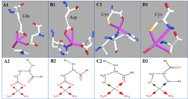
Four most prevalent zinc bidentation of standard amino acids in the wwPDB, with real structures on the top panel and schematic structures on the bottom. Panel A: Glutamate bidentates the zinc ion via two side chain oxygens. Count: 935; percentage: 33.7%. Example shown: PDB ID, 2E4T. Panel B: Aspartate bidentates the zinc ion via two side chain oxygens. Count: 935; percentage: 28.7%. PDB ID: 1RTQ. Panel C: Cysteine bidentates the zinc ion via one side chain sulfur and one back bone oxygen. Count: 153; percentage: 5.5%. PDB ID: 4FGL. Panel D: Cysteine bidentates the zinc ion via one side chain sulfur and one back bone nitrogen. Count: 57; percentage: 2.0%. PDB ID: 4A48.

Classifying a zinc fc‐shell with a compressed/super‐compressed angle into any of the previously canonical CG models will either create an outlier or add significant variance to subsequent analyses. Thus, we chose to separate compressed and super‐compressed angle containing zinc sites from normal zinc sites.

Separation of zinc fc‐shells into normal, compressed, and super‐compressed sets using randomForest

As mentioned earlier, Figure 2 shows the presence of compressed and super‐compressed angles between zinc fc‐shell ligands. Because of the overlapping distribution of the normal and compressed angles and the ligand and bidentation propensities of the ligands comprising these angles, we developed a randomForest classifier to deconvolute this overlap. Then, we used randomForest to classify zinc sites as normal, compressed, and super‐compressed groups based on three key factors: angles, bidentation status, and ligand residue type. The training data consisted of 16,375 sites (14,210 normal, 2087 compressed, and 78 super‐compressed) initially classified from the smallest angle. The total number is smaller than that previously mentioned (17,135) because we only used the nonoverlapping zinc sites as the training data. The out‐of‐bag error rate for the training data was 0.00 for the normal and compressed groups and 0.06 for the super‐compressed group. Importance measures showed that the most important feature is Angle 2 (with a score of 1836), followed by bidentation status (score 859), and Angle 6 (score 279). The reason that Angle 2 is the most important feature is because it is most likely to be the smallest angle because of the “largest‐sortedMiddle‐opposite” ordering of angles used. Angle 1 is always the largest angle and is, therefore, nearly impossible to be the smallest (i.e., special case where all angles are exactly equal). Angle 6 is the angle that is opposite to Angle 1 (e.g., has no ligand atoms in common with Angle 1), increasing its likelihood that it is the smallest angle. The bidentation status of ligands in the site showed its importance as expected from the histogram in Figure 3.

Sorting the six angles by largest‐sortedMiddle‐opposite makes them comparable across all geometries without introducing artificial scrambling. This was necessary for robustness in many of the analyses. As shown in Table 4 of ideal angles in this ordering, Angle 1 and Angle 6 in combination are highly distinct for different CGs. The middle four angles should be very close to each other except in the case of bva. Similar ordering for five‐ and six‐ligand CGs is shown in Supporting Information Tables S4 and S5.

After the removal of redundant sites, 6199 four‐ligand zinc fc‐shells were left for subsequent analyses. Applying the randomForest classifier to all of the zinc fc‐shells resulted in 4845, 1303, and 51 normal, compressed, and super‐compressed fc‐shells, respectively.

k‐Means clustering

In an initial failed attempt to cluster zinc fc‐shells using randomForest (results not shown), the ligand type and bond length showed very little influence in determining meaningful CGs, whereas the ligand–zinc–ligand bond angles and bidentation status were more important. Therefore, we applied k‐means clustering to the angles only to generate clusters of zinc sites. Note that clustering was done on the normal and compressed zinc sites separately, as otherwise the clustering was unstable (Supporting Information Fig. S3 and Supporting Information Tables S6 and S7).

Two measures were used in assessing cluster stability: the sum of absolute differences and the Jaccard index. The sum of absolute differences measures the differences between cluster centers over multiple clustering iterations. The Jaccard index evaluates the agreement of the set of actual zinc fc‐shells that are classified into the same cluster over multiple clustering iterations. Two measures were used to biologically validate the optimal k: Spearman's rho and P‐value between structural distances and functional distances of all cluster pairs. To make comparisons between all four values visually easier, we graphed the negative log of the P‐value and the max sum of absolute differences minus the sum of absolute differences with the Jaccard index and Spearman's rho. We expect the “true” k to have a local, simultaneous maximum for each of these four measures. Figure 7 shows how these four measures vary with respect to k for the normal group. k = 10 appears to be the consistent local maximization of all four measures. Figure 8 shows how these same measures vary with respect to k for the compressed group. In this case, k = 8 appears as the local maximization of all four measures.

Figure 7.

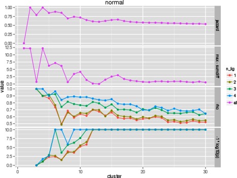
Comparison of k in k‐means clustering of the normal group with respect to four metrics.

Figure 8.

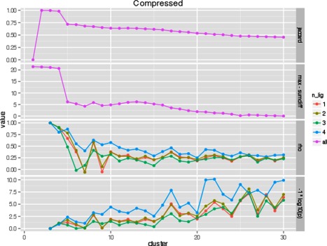
Comparison of k in k‐means clustering of the compressed group with respect to four metrics.

The angle statistics, average χ ² probabilities, and 3D structures of cluster representatives for the normal group are shown in Tables 5 and 7 and Supporting Information Figure S1, respectively. All of the standard deviations of the angles are much tighter in Table 5 than when we preselected the 10 canonical CG models for classification (Table 2). By comparing the angle means of each cluster to ideal angles in Table 4, Angle 1 of Clusters 4, 8, and 9 seems equivalent to 180°, because of folded normal distribution effect. Their Angle 6 is equivalent to 90°, 120°, and 180°, respectively. By taking into account their χ ² probabilities, which is a mathematical characterization of a cluster with respect to specific canonical CGs, and the 3D structure of the centroid zinc site, which is the visualization of the cluster, Clusters 4, 8, and 9 are assigned as Pyv, Bvp, and Spl. Similarly, Cluster 1 is assigned as Pyv, but distorted. Cluster 3 is assigned as Bva. Clusters 2, 5, 6, 7, and 10 are all subclasses of Tet. In fact, all of the canonical CGs find corresponding cluster(s) in Table 7 simply by using their maximal cluster average χ ² probabilities for assignment.

Table 5.

Mean and Standard Deviation of Angles for Each Cluster, Normal Group k = 10

Cluster	Size	Angle 1	Angle 2	Angle 3	Angle 4	Angle 5	Angle 6
1	331	150.0 ± 5.6	85.8 ± 7.0	93.8 ± 5.4	100.8 ± 4.4	109.2 ± 5.3	98.9 ± 7.1
2	741	123.4 ± 4.2	93.8 ± 4.9	101.8 ± 3.7	108.4 ± 3.9	115.2 ± 3.8	112.4 ± 4.6
3	213	135.5 ± 8.1	80.4 ± 7.1	91.1 ± 7.8	107.8 ± 8.2	122.3 ± 6.4	86.3 ± 9.6
4	381	167.4 ± 6.6	81.6 ± 6.0	87.4 ± 5.0	92.6 ± 4.5	99.0 ± 6.3	90.8 ± 8.6
5	205	138.8 ± 6.7	84.6 ± 7.6	92.8 ± 7.1	102.5 ± 6.2	113.8 ± 8.1	120.5 ± 8.2
6	1050	116.0 ± 2.9	103 ± 3.1	106.3 ± 2.1	108.9 ± 1.9	111.8 ± 2.1	110.5 ± 3.2
7	853	119.4 ± 3.0	100.8 ± 3.8	107.0 ± 2.9	111.2 ± 2.6	114.8 ± 2.5	101.3 ± 4.3
8	383	168.0 ± 6.7	80.4 ± 5.7	87.7 ± 4.1	93.2 ± 3.8	100.0 ± 5.6	116.9 ± 8.5
9	165	166.8 ± 8.1	79.6 ± 5.6	87.1 ± 3.5	92.3 ± 3.2	99.7 ± 6.2	155.3 ± 11.0
10	523	131.1 ± 4.9	94.9 ± 5.4	102.3 ± 3.9	108.5 ± 4.2	115.7 ± 4.8	96.7 ± 6.3

Table 7.

Average χ ² Probabilities of the Zinc Sites in Each CG for the Normal Group with k = 10. [Color table can be viewed in the online issue, which is available at wileyonlinelibrary.com.]

Cluster	Tet	Bva	Bvp	Pyv	Spl	Assignment
1	0.028	0.090	0.193	0.265	0.125	Pyv distorted
2	0.543	0.042	0.015	0.006	0.000	Tet
3	0.033	0.197	0.193	0.125	0.017	Bva
4	0.004	0.044	0.399	0.683	0.445	Pyv
5	0.096	0.071	0.047	0.013	0.002	Tet distorted
6	0.931	0.011	0.004	0.002	0.000	Tet
7	0.769	0.064	0.017	0.007	0.000	Tet
8	0.071	0.373	0.685	0.424	0.097	Bvp
9	0.009	0.063	0.461	0.585	0.564	Spl
10	0.218	0.149	0.082	0.070	0.009	Tet

The highest CG probability for each cluster is in red.

Tables 6 and 8 and Supporting Information Figure S2 are the angle statistics, average χ ² probabilities, and 3D structures of cluster representatives for the compressed group. Both mean angles and χ ² probabilities were assessed without considering the compressed angles, so that these novel structures could be related to canonical CGs with minimum effect from the compressed angles. Even by leaving out the compressed angle in calculating χ ² probabilities, most of the average χ ² probabilities are much lower than the normal group, which confirmed that they should not be directly classified into any of the canonical CGs. In contrast to the normal group, canonical CG assignment cannot simply use the maximal cluster average χ ² probabilities. In fact, such a simplistic assignment approach would have misassigned canonical CGs for five of the eight compressed clusters. There is also no highest probability on Tet, because Tet is the most geometrically symmetric structure, and having a compressed angle seems to disrupt this balance. By using all three pieces of information, most of the clusters can be viewed as distorted forms of the canonical CGs with one of the angles compressed. As for Cluster 5, it does not resemble any of the canonical CGs at all, except maybe a highly distorted Pyv, where it has three ligands on the same plane very close to each other, and the fourth ligand–zinc bond perpendicular to that plane.

Table 6.

Mean and Standard Deviation of Angles for Each Cluster, Compressed Group k = 8

Cluster	Size	Angle 1	Angle 2	Angle 3	Angle 4	Angle 5	Angle 6
1	186	128.2 ± 8.2	53.7 ± 6.1	92.1 ± 8.7	105.6 ± 6.1	115.0 ± 6.1	90.8 ± 9.4
2	141	155.9 ± 8.6	57.9 ± 6.4	86.6 ± 7.5	98.8 ± 6.4	112.0 ± 9.6	134.0 ± 10.3
3	275	153.0 ± 7.0	55.2 ± 5.4	88.2 ± 5.8	98.3 ± 5.2	105.7 ± 6.0	103.2 ± 9.2
4	84	128.5 ± 9.9	80.5 ± 7.6	92.3 ± 8.2	105.4 ± 9.5	116.4 ± 8.5	51.5 ± 4.8
5	126	130.8 ± 9.9	53.3 ± 6.3	75.2 ± 6.3	85.9 ± 6.7	100.7 ± 9.3	91.2 ± 11.9
6	91	157.1 ± 10.6	54.8 ± 7.2	77.0 ± 8.2	105.1 ± 12	129.1 ± 11.1	92.4 ± 14.5
7	53	159.8 ± 9.6	79.1 ± 9.0	86.7 ± 6.8	93.8 ± 6.8	103.1 ± 10.3	55.0 ± 6.3
8	209	139.6 ± 8.2	52.7 ± 5.6	83.4 ± 7.7	96.8 ± 7.0	111.1 ± 9.1	118.8 ± 6.7

Table 8.

Average χ ² Probabilities of the Zinc Sites in Each CG for the Compressed Group with k = 8 [Color table can be viewed in the online issue, which is available at wileyonlinelibrary.com.]

Cluster	Tet	Bva	Bvp	Pyv	Spl	Assignmenta
1	0.160	0.289	0.150	0.072	0.012	Bva with compressed 90
2	0.092	0.229	0.206	0.149	0.064	Spl with compressed 90
3	0.102	0.287	0.226	0.263	0.092	Distorted Pyv with compressed 90
4	0.074	0.159	0.090	0.062	0.015	Tet with compressed 109
5	0.031	0.146	0.154	0.184	0.060	New!
6	0.042	0.073	0.061	0.056	0.027	Pyv with compressed 90
7	0.022	0.313	0.313	0.362	0.330	Pyv with compressed opposite 90
8	0.112	0.133	0.197	0.050	0.005	Distorted Bvp with compressed 90

The highest CG probability for each cluster is in red, leaving out compressed angles in the probability calculation.

^aAssignments are based on average angles (Table 6) and χ ² probabilities with visual corroboration from the centroid zinc site (Supporting Information Fig. S2).

Now, if we use k‐means on both normal and compressed group together instead of separately, stability tests show that k = 10 and k = 14 are the potential optimal clustering numbers (Supporting Information Fig. S3). However, the Spearman's rho starts from a negative number as shown in Supporting Information Figure S3, indicating a much weaker structure–function relationship through clusters if we were to combine everything together. Also, angle statistics (Supporting Information Tables S6 and S7) show that all standard deviations, especially those with a compressed angle (Clusters 4, 5, 9, and 10 in Supporting Information Table S6, and Clusters 2, 3, 5, 9, and 12 in Table 7), are higher than when handling them separately. As shown in Supporting Information Table S6, the canonical CGs Spv and Bvp are very likely to be mixed together in Cluster 8 when using k = 10. Its discriminating position, Angle 6, is roughly the average of 90° (Spv) and 120° (Bvp), and the standard deviation is much higher compared with the other five angles. When using k = 14 as shown in Supporting Information Table S7, Spv and Bvp can be separated into Clusters 7 and 13, respectively. But the discriminating Angle 6 of both clusters have their means further from their ideal angles and the associated standard deviations are relatively high compared with when handling them separately (Table 5, Clusters 4 and 8). Restated, more zinc sites are misclassified and inappropriately associated if we cluster all zinc sites together rather than clustering zinc sites with all normal angles or with at least one compressed angle separately.

Functional analysis

To assess how the CG structures might influence the functional characteristics of zinc sites, the distances between clusters were calculated from both the ligand–zinc–ligand bond angles and InterProScan annotations that overlap a zinc–ligand (see Methods section). These distances were compared using Spearman's correlation (rho) and P‐value of the correlation.

The correlation ranged from 0.6 to 0.9 depending on the number of ligands required in the overlap between zinc binding sites and annotation sites identified by InterProScan. This high level of correlation implies that there is a definite link between the CG and the functional properties of a given zinc size. This is expected based on the sequence–structure–function tenet of structural biology; however, it is still beautiful to see.

Figure 9 shows the comparison of the dendrograms constructed from structural (Panel A) and functional (Panel B) distances for the normal group. Both structural and functional information created a hierarchical dendrogram cluster comprising normal k‐means Clusters 2 (nk2), nk5, nk6, nk7, and nk10 together, which are all Tet subclasses. Structurally, Bva (nk3) is the next closest k‐means cluster to the Tet super‐cluster, whereas functionally, Bva is closer to the core Tet super‐cluster than distorted Tet (nk5), which shows a relationship with another distorted CG cluster (nk1). As for k‐means clusters nk1, nk4, nk8, and nk9, distorted Pyv (nk1) and Pyv (nk4) are the first to cluster together in the structural dendrogram, closely followed by Bpv (nk8) and then Spl (nk9). Similarly, in functional dendrogram, Pyv (nk4) and Bpv (nk8) are grouped together and then with Pyv (nk1). Figure 10 shows the same comparison for compressed group. Compressed k‐means Cluster 4 (ck4) and ck7 are in a subgroup in both structural and functional dendrogram, and so are ck1 with ck5, and ck2 with ck8. These observations definitely indicate that there are certain structure–function propensities lying in these clusters that need to be further investigated. Also, the 3D structure of ck1 looks like an inverted Tet or Bva, and ck5 is a completely new CG that does not resemble any known CGs. They both are worth further investigation as well.

Figure 9.

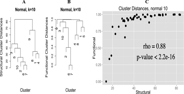
Hierarchical dendrogram (left) and Spearman's correlation (right) of structural and functional distances for k = 10 in the normal group.

Figure 10.

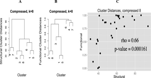
Hierarchical dendrogram (left) and Spearman's correlation (right) of structural and functional distances for k = 8 in the compressed group.

In addition to comparing the structural and functional distances directly, functional annotation enrichment was done for both the normal and compressed zinc sites. We used hypergeometric enrichment to compare the EC annotation and IPR annotations that overlap a zinc site in the normal and compressed groups relative to all of the annotated zinc sites.

We trimmed the EC numbers to the second digit as annotations for enrichment calculations. The EC numbers are enriched in either the compressed or normal group, but not both (Supporting Information Table S14). The most enriched enzyme classes in the normal group are 4.2 (carbon oxygen lyases), followed by 2.1 (transferases transferring one‐carbon groups), 3.4 (peptidases), and 4.4 (carbon sulfur lyases). Comparatively, in the compressed group, the most enriched enzyme classes are 1.7 (oxidoreductases acting on other nitrogenous compounds as donors), 0 (no EC number), 3.2 (glycosylases), 1.16 (oxidoreductases oxidizing metal ions), and 2.4 (glycosyltransferases).

Similarly, a number of InterPro annotations are enriched in either the normal or compressed group, but not both (Supporting Information Table S15). In fact, many of the InterPro annotations in the normal zinc sites are not present at all in the compressed sites, but all sites are only in the normal group, including the most highly enriched annotations such as C2H2 zinc fingers (IPR015880 and IPR007087) and glycoside hydrolase (IPR027291, IPR015341, and IPR028995). Many of the other highly enriched annotations in normal have only a few sites in the compressed group, including carbonic anhydrase (IPR018338, IPR023561, and IPR018443) and PHD‐type zinc fingers (IPR013083, IPR019787, and IPR019786).

The compressed‐specific annotations included pollen allergen (IPR001778 and IPR002914), as well as protein of unknown function (IPR010281). Other highly enriched annotations include immunoglobulin domains (IPR013783, IPR007110, and IPR013106), ferritin (IPR009078 and IPR012347), super‐antigens (IPR016091 and IPR013307), and staphylococcal/streptococcal toxins (IPR006126, IPR006173, and IPR006177).

These results imply that although there are many functions that can be performed by both normal and compressed CGs, there are some that seem to be specific to one type or the other.

DISCUSSION

Previous works have attempted to characterize zinc binding in metalloproteins by considering only canonical zinc CGs that have been previously observed and explained by coordination chemistry. However, when these expectations of canonical CGs are applied to zinc ions bound by proteins, many zinc sites are classified as outliers or are misclassified with respect to CG (see Table 2, and Andreini et al.22). Our analysis of ligand–zinc–ligand bond angles, where the best fc‐shell is determined from only previously characterized zinc–ligand bond lengths, and then the ligand–zinc–ligand angles examined, showed the presence of angles below 58° (compressed) and 38° (super‐compressed). As these angles are incompatible with any previously characterized canonical CG, they implied the existence of unknown CGs. Many, but not all of the compressed and super‐compressed angles seem to contain bidentate ligands (wherein two of the ligands to the zinc atom are from the same amino acid residue or molecule) or non‐amino acid ligands. This points to the need for less‐biased methods for determining zinc CGs in proteins.

What is especially interesting is that it is not possible to organize all of the CGs using only the angle information. Clustering all of the zinc sites using only the sorted angles does not lead to stable clusters (Supporting Information Fig. S3 and Supporting Information Tables S6 and S7). This aspect of the CG detection methodology (in combination with using known bond length's mean and standard deviations) leads to our method being less biased than previous methods; however, there is still a bias. The sites must still be classified as either normal or compressed prior to clustering on the angles. But this classification is based on direct observations of the angle distributions in the dataset and not on prior belief of what is in the dataset.

Following the clustering of the normal and compressed zinc sites, assignment to canonical CGs was made based on agreement with their expected angles. The normal sites fit canonical CGs very well, as is expected. An attempt was made to relate the compressed CGs to canonical CGs using a combination of criteria including χ ² probability calculations after removing the compressed angle to remove that as a source of bias. The assignment to canonical CGs in this case is still a bit of a misnomer, as most of these severely compressed versions of canonical CGs have not been described in the literature. From this perspective, they can be viewed as novel CGs. However, we took the conservative approach of simply describing them as large distortions of the canonical CGs. We have also labeled the compressed CG (Cluster 5 of the compressed group) that appears completely distinct from all of the other canonical CGs as truly “novel.”

To allay suspicions that these compressed angles are the result of experimental artifacts, such as whether or not it is just due to the uncertainty of the X‐ray experiment, we calculated the average of the b‐factors of the ligands composing the compressed angle versus normal angles. As shown in Supporting Information Figure S4, there is no significant difference between their composing ligands. There is literature suggesting that some of the compressed angles are a result of a phenomenon called a carboxylate shift,41 which is a thermodynamic mechanism enzymes employ to sustain the CG when binding and leaving a substrate. However, no one has systematically examined this phenomenon in terms of metal's CG in the wwPDB. Also, a simple mechanism could not cover all instances, such as the bidentation caused by ligation of cysteine's backbone and side‐chain together.

The compressed and novel CGs beg the question: why have they not been previously reported? One answer is that until recently there has not existed enough example structures for them to be reliably observed even with our less‐biased characterization methods. Figure 11 shows how the number of compressed zinc sites has increased proportionately with the growth of the wwPDB. It is only within the past 10 years that enough compressed sites existed in the wwPDB for a rigorous study to observe and detect them. More importantly, however, is the fact that even with a relatively large fraction of compressed sites, an analysis that considers only the canonical CGs from previously identified zinc coordinations and bonding structures will remove compressed sites from the analysis as outliers. This is exemplified by the work of Andreini et al., MetalPDB,22 where the summary of zinc metal showed that the outlier category had the largest number of instances. Figure 11 shows that there should have been more than enough compressed sites to be detectable; however, there were no compressed sites reported by Andreini et al. There was a number of outliers noted in their work. Some of the outliers reported by Andreini et al. were likely zinc sites with compressed CGs, but because their analysis considered only “normal” zinc CGs, the compressed CGs were overlooked and not reported. This directly underscores the need for less‐biased analyses of metal CGs in proteins so that these previously described CGs are not overlooked or merely classed as outliers and completely removed from an analysis.

Figure 11.

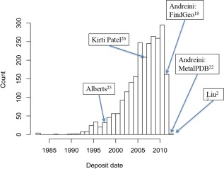
Analysis of the deposition history of the March 2013 wwPDB zinc metalloprotein entries with compressed angles. Publication date of the key references are indicated on the graph.

These compressed sites also show enriched functionality relative to all of the sites, suggesting that there are particular functions or enzyme classes that are preferentially compressed. The correspondence between CG cluster distances from angles and cluster distances from functional annotation further emphasize the functional importance of the compressed and novel CGs. However, it should also be emphasized that it is difficult from this work to assign functionality to particular normal or compressed clusters, as multiple clusters seem to share functionality. We see two possible explanations: (a) presence of false positives in associating function with the zinc sites and (b) potential existence of zinc metalloproteins with multiple zinc‐coordinating CG conformations, but where the X‐ray crystal structure freezes out just one conformation. Improvements in functional annotation methods will be required to address these short‐comings, including: (i) the development of better annotating hidden Markov models to better relate zinc binding site detected from protein sequence to specific protein functions and (ii) the development of better methods that relate overlapping protein regions with respect to protein functions. Dealing with the second explanation may only be addressed by NMR studies42 and/or newer combined quantum mechanical, molecular mechanical, molecular dynamics simulations.43

CONCLUSIONS

We have developed a less‐biased approach for the classification of zinc binding sites with respect to CG that allows for the detection of novel CGs. From one perspective, we have detected eight novel CGs that contain compressed angles and cannot easily be classified into one of the canonical CGs. From another perspective, seven of these eight novel CGs can be viewed as highly distorted versions of the canonical CGs; however, this perspective may be considered as simply trying to push a square peg into a round hole. From either perspective, one of the compressed CGs appears to be truly novel and distinct from all canonical CGs by every probabilistic, angle comparison, and visual inspection criteria we could use. As the wwPDB continues to grow, additional distorted or novel CGs may become detectable; however, we will only be able to detect these previously undetected CGs by using an unsupervised clustering approach such as the one described in this article rather than applying a supervised classification method based on “known” CGs, which has been the method of choice up to this point in time. In other words, we will be able to detect these previously undetected CGs only if we stop assuming that we already know what a dataset contains before analyzing it.

Supporting information

Supporting Information

REFERENCES

- 1. Keilin D, Mann T. Carbonic anhydrase. Nature 1939;144:442–443. [Google Scholar]
- 2. Tan D, Zhou M, Kiledjian M, Tong L. The ROQ domain of Roquin recognizes mRNA constitutive‐decay element and double‐stranded RNA. Nat Struct Mol Biol 2014;21:679–685. [DOI] [PMC free article] [PubMed] [Google Scholar]
- 3. Miller J, McLachlan AD, Klug A. Repetitive zinc‐binding domains in the protein transcription factor IIIA from Xenopus oocytes. EMBO J 1985;4:1609–1614. [DOI] [PMC free article] [PubMed] [Google Scholar]
- 4. Elrod‐Erickson M, Benson TE, Pabo CO. High‐resolution structures of variant Zif268‐DNA complexes: implications for understanding zinc finger‐DNA recognition. Structure 1998;6:451–464. [DOI] [PubMed] [Google Scholar]
- 5. Carrigan CN, Poulter CD. Zinc is an essential cofactor for type I isopentenyl diphosphate:dimethylallyl diphosphate isomerase. J Am Chem Soc 2003;125:9008–9009. [DOI] [PubMed] [Google Scholar]
- 6. Rowlett RS. Structure catalytic mechanism of beta‐carbonic anhydrases. Subcell Biochem 2014;75:53–76. [DOI] [PubMed] [Google Scholar]
- 7. Bellomo E, Massarotti A, Hogstrand C, Maret W. Zinc ions modulate protein tyrosine phosphatase 1B activity. Metallomics 2014;6:1229–1239. [DOI] [PubMed] [Google Scholar]
- 8. Jiang LJ, Vasak M, Vallee BL, Maret W. Zinc transfer potentials of the alpha‐ and beta‐clusters of metallothionein are affected by domain interactions in the whole molecule. Proc Natl Acad Sci USA 2000;97:2503–2508. [DOI] [PMC free article] [PubMed] [Google Scholar]
- 9. Takeda A. Zinc homeostasis and functions of zinc in the brain. Biometals 2001;14:343–351. [DOI] [PubMed] [Google Scholar]
- 10. Rink L, Haase H. Zinc homeostasis and immunity. Trends Immunol 2007;28:1–4. [DOI] [PubMed] [Google Scholar]
- 11. Fukada T, Yamasaki S, Nishida K, Murakami M, Hirano T. Zinc homeostasis and signaling in health and diseases: zinc signaling. J Biol Inorg Chem 2011;16:1123–1134. [DOI] [PMC free article] [PubMed] [Google Scholar]
- 12. Milne A, Landing W, Bizimis M, Morton P. Determination of Mn, Fe, Co, Ni, Cu, Zn, Cd and Pb in seawater using high resolution magnetic sector inductively coupled mass spectrometry (HR‐ICP‐MS). Anal Chim Acta 2010;665:200–207. [DOI] [PubMed] [Google Scholar]
- 13. Wang C, Li B, Ao J. Separation and identification of zinc‐chelating peptides from sesame protein hydrolysate using IMAC‐Zn(2)(+) and LC‐MS/MS. Food Chem 2012;134:1231–1238. [DOI] [PubMed] [Google Scholar]
- 14. Andreini C, Bertini I, Rosato A. Metalloproteomes: a bioinformatic approach. Acc Chem Res 2009;42:1471–1479. [DOI] [PubMed] [Google Scholar]
- 15. Andreini C, Bertini I, Rosato A. A hint to search for metalloproteins in gene banks. Bioinformatics 2004;20:1373–1380. [DOI] [PubMed] [Google Scholar]
- 16. Maret W. Zinc biochemistry: from a single zinc enzyme to a key element of life. Adv Nutr 2013;4:82–91. [DOI] [PMC free article] [PubMed] [Google Scholar]
- 17. Andreini C, Bertini I, Cavallaro G, Holliday GL, Thornton JM. Metal‐MACiE: a database of metals involved in biological catalysis. Bioinformatics 2009;25:2088–2089. [DOI] [PubMed] [Google Scholar]
- 18. Andreini C, Cavallaro G, Lorenzini S. FindGeo: a tool for determining metal coordination geometry. Bioinformatics 2012;28:1658–1660. [DOI] [PubMed] [Google Scholar]
- 19. Berman H, Henrick K, Nakamura H. Announcing the worldwide Protein Data Bank. Nat Struct Biol 2003;10:980. [DOI] [PubMed] [Google Scholar]
- 20. Castagnetto JM, Hennessy SW, Roberts VA, Getzoff ED, Tainer JA, Pique ME. MDB: the Metalloprotein Database and Browser at The Scripps Research Institute. Nucleic Acids Res 2002;30:379–382. [DOI] [PMC free article] [PubMed] [Google Scholar]
- 21. Harding MM, Hsin KY. Mespeus–a database of metal interactions with proteins. Methods Mol Biol 2014;1091:333–342. [DOI] [PubMed] [Google Scholar]
- 22. Andreini C, Cavallaro G, Lorenzini S, Rosato A. MetalPDB: a database of metal sites in biological macromolecular structures. Nucleic Acids Res 2013;41(Database issue):D312–D319. [DOI] [PMC free article] [PubMed] [Google Scholar]
- 23. Andreini C, Bertini I. A bioinformatics view of zinc enzymes. J Inorg Biochem 2012;111:150–156. [DOI] [PubMed] [Google Scholar]
- 24. Zastrow ML, Pecoraro VL. Designing hydrolytic zinc metalloenzymes. Biochemistry 2014;53:957–978. [DOI] [PMC free article] [PubMed] [Google Scholar]
- 25. Alberts IL, Nadassy K, Wodak SJ. Analysis of zinc binding sites in protein crystal structures. Protein Sci 1998;7:1700–1716. [DOI] [PMC free article] [PubMed] [Google Scholar]
- 26. Patel K, Kumar A, Durani S. Analysis of the structural consensus of the zinc coordination centers of metalloprotein structures. Biochim Biophys Acta 2007;1774:1247–1253. [DOI] [PubMed] [Google Scholar]
- 27. Liu Z, Wang Y, Zhou C, Xue Y, Zhao W, Liu H. Computationally characterizing and comprehensive analysis of zinc‐binding sites in proteins. Biochim Biophys Acta 2014;1844:171–180. [DOI] [PubMed] [Google Scholar]
- 28. Breiman L. Random forests . Mach Learn 2001;45:5–32. [Google Scholar]
- 29. Breiman L. Manual–setting up, using, and understanding random forests V4. 0. 2003. Available at: https://www.stat.berkeley.edu/~breiman/Using_random_forests_v4.0.pdf
- 30. Hartigan JA, Wong MA. Algorithm AS 136: a k‐means clustering algorithm. Appl Stat 1979; 28:100–108. [Google Scholar]
- 31. Jones P, Binns D, Chang H‐Y, Fraser M, Li W, McAnulla C, McWilliam H, Maslen J, Mitchell A, Nuka G. InterProScan 5: genome‐scale protein function classification. Bioinformatics 2014;30:1236–1240. [DOI] [PMC free article] [PubMed] [Google Scholar]
- 32. Murtagh F, Legendre P. Ward's hierarchical agglomerative clustering method: which algorithms implement Ward's criterion? J Classif 2014;31:274–295. [Google Scholar]
- 33. Murtagh F. Multidimensional clustering algorithms. Compstat lectures, Vol. 4. Vienna: Physika Verlag; 1985. [Google Scholar]
- 34. Kanehisa M, Goto S, Sato Y, Furumichi M, Tanabe M. KEGG for integration and interpretation of large‐scale molecular data sets. Nucleic Acids Res 2012;40 :D109–D114. [DOI] [PMC free article] [PubMed] [Google Scholar]
- 35. Harding MM. Small revisions to predicted distances around metal sites in proteins. Acta Crystallogr D Biol Crystallogr 2006;62:678–682. [DOI] [PubMed] [Google Scholar]
- 36. Tamames B, Sousa SF, Tamames J, Fernandes PA, Ramos MJ. Analysis of zinc‐ligand bond lengths in metalloproteins: trends and patterns. Proteins 2007;69:466–475. [DOI] [PubMed] [Google Scholar]
- 37. Harding MM, Nowicki MW, Walkinshaw MD. Metals in protein structures: a review of their principal features. Crystallogr Rev 2010;16:247–302. [Google Scholar]
- 38. Onoa B, Moreno V. Nickel (II) and copper (II)–l‐cysteine, l‐methionine, l‐tryptophan‐nucleotide ternary complexes. Transit Metal Chem 1998;23:485–490. [Google Scholar]
- 39. Roe RR, Pang Y‐P. Zinc's exclusive tetrahedral coordination governed by its electronic structure. J Mol Model 1999;5:134–140. [Google Scholar]
- 40. McCall KA, Huang C, Fierke CA. Function and mechanism of zinc metalloenzymes. J Nutr 2000;130:1437S–1446S. [DOI] [PubMed] [Google Scholar]
- 41. Sousa SF, Fernandes PA, Ramos MJ. The carboxylate shift in zinc enzymes: a computational study. J Am Chem Soc 2007;129:1378–1385. [DOI] [PubMed] [Google Scholar]
- 42. Huang YJ, Montelione GT. Structural biology: proteins flex to function. Nature 2005;438:36–37. [DOI] [PubMed] [Google Scholar]
- 43. Hofer TS, Randolf BR, Rode BM. Molecular dynamics simulation methods including quantum effects In: Canuto S, editor. Solvation effects on molecules and biomolecules. Challenges and advances in computational chemistry and physics. The Netherlands: Springer; 2008. pp 247–278. [Google Scholar]
Associated Data
This section collects any data citations, data availability statements, or supplementary materials included in this article.
Supplementary Materials