

Abstract
Motivation: DNA sequencing of multiple samples from the same tumor provides data to analyze the process of clonal evolution in the population of cells that give rise to a tumor.
Results: We formalize the problem of reconstructing the clonal evolution of a tumor using single-nucleotide mutations as the variant allele frequency (VAF) factorization problem. We derive a combinatorial characterization of the solutions to this problem and show that the problem is NP-complete. We derive an integer linear programming solution to the VAF factorization problem in the case of error-free data and extend this solution to real data with a probabilistic model for errors. The resulting AncesTree algorithm is better able to identify ancestral relationships between individual mutations than existing approaches, particularly in ultra-deep sequencing data when high read counts for mutations yield high confidence VAFs.
Availability and implementation: An implementation of AncesTree is available at: http://compbio.cs.brown.edu/software.
Contact: braphael@brown.edu
Supplementary information: Supplementary data are available at Bioinformatics online.
1 Introduction
Cancer is a disease resulting from somatic mutations that accumulate during an individual’s lifetime and lead to uncontrolled growth of a collection of cells into a tumor. The clonal theory of cancer (Nowell, 1976) predicts that all cells within a tumor have descended from a single founder cell and that subsequent clonal expansions occur from additional advantageous mutations. As a result, the cells within a tumor may differ in their complement of somatic mutations, with each cell being a descendant of a clone from a clonal expansion (Fig. 1A). High-coverage sequencing of tumor genomes allows one to study this intra-tumor heterogeneity by measuring the frequencies of mutations within a tumor (Ding et al., 2012; Nik-Zainal et al., 2012; Shah et al., 2012). Characterization of intra-tumor heterogeneity and inference of the clonal evolutionary history of somatic mutations within a tumor provide useful insight in the tumor’s development and may help inform treatment.
Fig. 1.

Model for clonal evolution and inference. (A) An example of the evolution of a tumor containing seven distinct clones. Passenger mutations (white) occurring before the first clonal expansion will be indistinguishable from mutations driving the growth of the founding clone (light blue). Each subsequent mutation (green, purple, dark blue, orange, red and tan) creates a new clone. (B) Three sequenced tumor samples. Some clones may no longer exist at the time of sequencing (orange). Samples 1 and 2 each contain a single clone (purple and blue respectively), whereas Sample 3 is a mixture of three clones (light blue, red and tan). (C) The frequency matrix F observed for the three sequenced samples indicated in part B. (D) The usage matrix U and clonal matrix B that generate F. Even though some clones existing at the current time may not be contained within a sequenced sample (green), their existence in the evolutionary history of the tumor may be recovered. (E) Tree of the inferred tumor clones. Solid black edges are the clonal tree T corresponding to the clonal matrix B. Gray dashed edges indicate internal vertices used in the mixing of some sample. The number next to each clone in each sample indicates the fraction of cells in the sample from that clone. (F) The ancestry graph for the observed data. The bold arcs indicate the spanning arborescence corresponding to T
Somatic mutations are typically measured in human solid tumors only at a single time point, when the patient undergoes surgery. Therefore, clonal evolution is not directly observed and one is faced with the problem of inferring the ancestral relationships between cells in a tumor from measurements at one time point. This is the problem of phylogenetic tree reconstruction, a well-studied problem. The direct application of phylogenetic methods requires that we measure mutations in individual cancer cells that correspond to the leaves (species) of the phylogenetic tree. However, because of technical limitations and financial considerations, single-cell sequencing of tumors remains uncommon (Navin, 2014; Wang et al., 2014) with nearly all cancer sequencing studies—including studies such as TCGA and ICGC—sequencing a small number of samples from a bulk tumor, each containing potentially millions of cells. Thus, the data one obtains represent the mutations in a mixture of cells with potentially distinct evolutionary histories.
Given sequencing data from a single sample, a number of methods have been developed to determine the set of clones and their frequencies in a tumor. Some methods analyze changes in the variant allele frequencies (VAFs) of single-nucleotide mutations; i.e. the fraction of tumor cells that contain each mutation (Miller et al., 2014; Roth et al., 2014). Other approaches analyze differences in read depth due to copy number aberrations (Oesper et al., 2013, 2014). More detailed inference of clonal evolution from a single sample requires additional assumptions about the evolutionary process, such as parsimony (Hajirasouliha et al., 2014; Strino et al., 2013).
Recently, several studies have sequenced multiple samples from the same tumor. These studies measure somatic mutations in multiple spatially distinct regions from the same tumor at a single time point (Gerlinger et al., 2012, 2014; Newburger et al., 2013; Zhang et al., 2014) or measure a tumor at multiple time points (Schuh et al., 2012). Multi-sample data allow for the direct observation of branched evolution when mutations are present in only a subset of the sequenced samples. Although standard phylogenetic techniques have been used to construct trees that relate these samples, such trees do not directly show the relationships between mutations, as each sequenced sample may itself be a heterogeneous mixture of cells (Fig. 1B).
Several methods have recently been introduced to infer tumor composition and evolution from VAFs of somatic mutations in multi-sample sequencing data. Clomial (Zare et al., 2014) infers the set of clones present in the tumor and their frequencies in each sample but does not describe the evolutionary relationships between the clones. Three recent approaches infer a tree describing the evolutionary history of a tumor. PhyloSub uses a Bayesian approach to sample trees using a tree-structured process (Jiao et al., 2014). CITUP (Malikic et al., 2015) enumerates all rooted trees and for each one solves a quadratic program. LICHeE, which recently appeared on the arXiv preprint server (Popic et al., 2014), uses a graph construction similar to one we describe below but does not provide a rigorous mathematical justification for it. All these approaches are data driven and focus on the construction and optimization of models that minimize the error between the observed and inferred mutation frequencies. However, they do not address the combinatorial structure of the problem. Stated more directly: given error-free VAF data, under what conditions is it possible to reconstruct the clonal evolution of a tumor?
We formalize the problem of reconstructing the clonal evolution of a tumor as the VAF factorization problem (VAFFP). The input to this problem are the VAFs for individual somatic mutations from one or more samples. The problem is to determine the composition of each sample, including the number and proportion of clones in each, and a tree that describes the ancestral relationships between all clones under the infinite sites (perfect phylogeny) assumption.
We prove necessary and sufficient conditions for the VAFFP to have a solution in the case of error-free data. Using these conditions, we provide a combinatorial characterization of the space of all solutions. We show that the VAFFP is NP-complete and give an integer linear programming formulation. We extend the characterization and formulation to noisy data and use a graph clustering approach to cluster mutations by their putative ancestral relationships. We show that our resulting AncesTree algorithm is better able to identify ancestral relationships between individual mutations than existing approaches on simulated data. On real data, we highlight the advantages of our probabilistic model by comparing whole-exome and deep sequencing data from the same tumor, identifying successive clonal expansions and diverse mixing of clones within sequenced samples.
2 Methods
2.1 Model for clonal evolution and inference
In this section, we describe a model for the accumulation of single-nucleotide somatic mutations in a tumor and the generation of sequencing data from the tumor. This leads us to the definition of the VAFFP at the conclusion of the section.
Following the clonal theory of cancer, we assume that all cancer cells in a tumor are descendants of a single founding clone; i.e. the tumor is monoclonal. In this work, we model only somatic single-nucleotide mutations and assume that these are unaffected by copy number aberrations or rearrangements in the cancer genome. We will use mutation to refer specifically to these events. We assume, as in previous work (Hajirasouliha et al., 2014; Jiao et al., 2014; Malikic et al., 2015), that mutations satisfy the infinite sites assumption, which states that a mutation occurs at a single genomic position, or locus, at most once during the clonal evolution of the tumor. We encode the state of a specific locus in a clone as a binary value—where 1 indicates a somatic mutation at that position and 0 indicates no mutation. Thus, each clone corresponds to a binary vector in , where n is the total number of loci affected by mutations.
Under these assumptions, the ancestral relationships between clones are described by a phylogenetic tree where (i) vertices represent different tumor clones that have existed during the tumor’s evolution and (ii) edges represent the direct ancestral relationships between clones and are labeled with the mutation(s) that distinguishes the child from its parent (Fig. 1A). In practice, we will group individual mutations into sets that satisfy the second condition and consider these as individual mutations. Thus, we describe the mutational process that produced a tumor by an n-clonal tree T, which we define as follows.
Definition 1 —
A rooted tree T on n vertices is an n-clonal tree for a mutation set provided each edge is labeled with exactly one mutation from and no mutation appears more than once in T. Let be the set of all n-clonal trees.
We denote the root vertex of an n-clonal tree by vr where is the mutation that does not label any edge in T. We denote the remaining vertices by vj where is the mutation on the last edge of the path from vr to vj. Note that the set of mutations present in a clone vj is the set of mutations of all vertices on the path from vr to vj. The root vertex vr contains only mutation r and thus represents the founding clone.
Alternatively, we may describe the n-clonal tree T by an n × n binary matrix B. We label the vertices of T by binary row vectors indicating the mutations present in each vertex (clone). Each vertex vj corresponds to a binary row vector with 1’s at the position and positions indicated by the edge labels of the unique path from vr to vj and 0’s at the remaining positions. Let B be the n × n binary matrix whose row is . As the mutations adhere to the infinite sites assumption, it follows that B is a perfect phylogeny matrix (Gusfield, 1991). That is, for a column j of B, let I(j) be the positions of the 1 entries. Then for any pair of columns j and k of B either I(j) and I(k) are disjoint, or one contains the other.
Not every n × n perfect phylogeny matrix corresponds to a n-clonal tree T. For example, a perfect phylogeny matrix may have a row and/or column of all 0’s or have duplicated rows and/or columns. We define a subset of n × n perfect phylogeny matrices, which we call n-clonal matrices that are in 1-1 correspondence with n-clonal trees T.
Definition 2 —
A matrix is an n-clonal matrix provided:
There exists exactly one such that .
For each there exists exactly one such that and .
bjj = 1 for all .
Let be the set of all n-clonal matrices.
The second condition above ensures that every n-clonal matrix is a perfect phylogeny matrix. We have the following lemmas, which we prove in the Supplementary Appendix.
Lemma 1 —
There is a one-to-one correspondence between and .
Lemma 2 —
Any has rank n.
Figure 1D and E show a clonal matrix together with its corresponding clonal tree.
2.1.1 Measurement of clonal trees
We do not directly observe the clonal tree T relating the clones in a tumor. Moreover, unless we perform single-cell sequencing, we do not directly measure the presence/absence of mutations in individual clones. Rather, each sequenced sample is a mixture of cancer cells (clones) and normal cells. We obtain VAFs or the fraction of reads covering a position that indicate the variant/mutation at each of the mutation sites in each of the samples. The VAF for a mutation is proportional to the cellular prevalence or fraction of cells in the sample that contain the mutation. Suppose we sequence m samples from a tumor with n mutations sites. Our observations are then described by an m × n frequency matrix , where fpi indicates the observed VAF in sample p for the mutation (Fig. 1C).
The observed mutation frequencies (entries of F) are related to the tree T by the proportions of normal cells and tumor clones that define the mixture in each sample. We define an m × n usage matrix , where upi indicates the fraction of cells in sample p that come from clone vi, as follows.
Definition 3 —
An m × n matrix is a usage matrix provided and . Let be the set of all m × n usage matrices U.
Since each sequenced sample is a mixture of clones from T with proportions defined in the usage matrix U, the observed frequency matrix satisfies
| (1) |
The coefficient arises because, by the infinite sites assumption, all mutations are heterozygous, and thus each .
Assuming no errors in F, our goal is to find U and B satisfying (1). We define this problem as follows (Fig. 1D).
Variant Allele Frequency Factorization Problem —
Given an m × n frequency matrix F, find a usage matrix and a clonal matrix such that .
Without loss of generality, we assume that the rows and columns of any frequency matrix F are distinct, as duplicated rows or columns can be collapsed.
The VAFFP formalizes and generalizes several problems that have previously been considered in the literature. In the case of m = 1 sample, Strino et al. (2013) and Hajirasouliha et al. (2014) address the problem of minimizing the number of non-zero entries in U, with Strino et al. (2013) breaking ties in favor of solutions whose clonal trees have minimum depth. Hajirasouliha and Raphael (2014) introduce the Perfect Phylogeny Mixture Problem, which can be described as a variant of the VAFFP where F is binary (a mutation is either observed or not) and additional constraints are placed on the usage matrix U. In the case of m > 1 sample, PhyloSub (Jiao et al., 2014) and CITUP (Malikic et al., 2015) minimize the distance between the observed and inferred F while adhering to the VAFFP. Below we provide further details of the relationships between the various approaches.
2.2 Solving the VAFFP
In this section, we derive a characterization of the solutions of the VAFFP (Theorem 1 below) as constrained spanning arborescences of a directed acyclic graph (DAG) called the ancestry graph (Definition 4 below). From this characterization, we prove that the VAFFP is NP-complete (Theorem 2 below) and give an exact algorithm for solving the problem.
2.2.1 A necessary condition and the ancestry graph
We say that B (or T) generates F if and only if there exists a matrix such that . To obtain a characterization of all solutions of the VAFFP, we first define several properties that relate the observed values of F to any clonal tree T that generates F.
We start by observing that any T induces a partial ordering on the vertices. That is, for if and only if vertex vj is an ancestor of vertex vk. Conversely, we say that j and k are incomparable if and only if neither vj nor vk is an ancestor to the other. Because B is a perfect phylogeny matrix, there is a partial order on the columns of B (Gusfield, 1997). That is, for , we have if and only if . Similarly, j and k are incomparable if and only if and . From Lemma 1, it follows that if and only if for all . Therefore, we will use to denote either one. We now prove the following condition.
Ancestry Condition —
If T generates F and then for all samples .
Proof —
Since and are equivalent, then . Moreover, because every entry in U is non-negative, we have the following for all samples :
The contrapositive of the Ancestry Condition for two distinct samples yields the following corollary which is equivalent to the ‘crossing rule’ stated in Jiao et al. (2014).
Corollary 1 —
If T generates F and there exist samples and mutations such that fpj > fpk and fqj < fqk then j and k are incomparable.
We summarize all possible ancestral relationships between mutations in F in a graph (Fig. 1F).
Definition 4 —
Given an m × n frequency matrix F, the ancestry graph is the directed graph with vertices and arcs .
The following observation which will be useful in the following section.
Observation 1 —
If all columns of a frequency matrix F are distinct then the ancestry graph G is a DAG.
A spanning arborescence of the ancestry graph G is a subgraph with , such that there exists a unique path from the root vertex vr to every vertex .
Lemma 3 —
If T generates F then T is a spanning arborescence of G.
Proof —
Let T be a tree that generates F. Suppose for the sake of contradiction that T is not a spanning arborescence of G. Thus, there exists an edge (vj, vk) in T with such that . By definition of A there must exist such that fpj < fpk and fqj > fqk. By Corollary 1, j and k are incomparable—a contradiction. Hence, T must be a spanning arborescence of G.
If an ancestry graph does not have a spanning arborescence then there exists no tree T that generates F. Checking whether G has a spanning, arborescence can be done in time since by definition A contains all transitive arcs. Figure 2A shows an example of a frequency matrix whose ancestry graph has no spanning arborescence. Furthermore, not all spanning arborescences T of G generate F. Figure 2B shows such an example, where the matrix U obtained from T and F has negative entries and thus is not a usage matrix. Hence, the existence of a spanning arborescence in G is a necessary but not a sufficient condition for a solution to the VAFFP.
Fig. 2.

Spanning arborescences of the ancestry graph. (A) F cannot be factorized as its ancestry graph does not admit a spanning arborescence. (B) Red arcs indicate a spanning arborescence T of the ancestry graph of F with corresponding matrix B. B does not generate F as the matrix
2.2.2 The sum condition and sufficiency
In the previous section, we saw that the ancestry condition is not sufficient to produce a solution to the VAFFP. Sufficiency will be obtained through a second condition, which we refer to as the sum condition. This condition was stated as the ‘sum rule’ in Jiao et al. (2014), also appears in Strino et al. (2013) and Malikic et al. (2015), and a special case was called the ‘children sum to parents’ condition in Hajirasouliha et al. (2014). Given a clonal tree T, let denote the children of a vertex vj in T.
Sum Condition —
If T generates F then for all samples and mutations ,
(2)
See the Supplementary Appendix for the proof of the sum condition.
For a clonal tree T, sample p and mutation j, we define the deficit . Thus, the Sum Condition states that if T generates F, then the deficit dpj is non-negative for all samples p and mutations j. It turns out that the deficits for all samples and mutations determine the matrix U. In particular, we have the following lemma.
Lemma 4 —
Given an m × n frequency matrix F and an n-clonal matrix B, the m × n matrix defined as
(3) is the unique matrix such that .
Proof —
Lemma 2 tells us that there is a unique such that . It suffices to show that for any sample p and mutation j. Let T be the corresponding clonal tree of B and . Since bkj = 1 for all , we have
Note that I(j) is the set of indices of all vertices in the subtree rooted at vj in T including vj itself. Since T is a tree, for any with , we have . Thus, in the last line of the above derivation, we subtract fpl exactly once for all vertices that are in the subtree rooted at vj. The set of such vertices is . Hence,
Note that by Lemma 2, any is full rank and therefore invertible. Therefore, for any frequency matrix F, there is a unique such that , namely . Thus, the above lemma gives an explicit formula for the entries of . For the single sample case, a similar formula was derived by Strino et al. (2013). However, instead of using this formula to infer the usage vector, the authors use back substitution. Jiao et al. (2014) and Malikic et al. (2015) also describe a recursive formula relating the frequencies and usages. Moreover, dpj = 0 is equivalent to the ‘children sum to parents’ condition in Hajirasouliha et al. (2014) and the ‘non-populated clone’ condition in Strino et al. (2013). In this case upj = 0, which implies that the clone vj is not present (or mixed) in sample p.
The matrix U defined by Equation (3) has non-negative entries whose rows sum to at most 1 and thus is a valid usage matrix precisely when the deficits are non-negative. This in turn happens when F satisfies the sum condition [Equation (2)]. Combining these results, we obtain the following lemma.
Lemma 5 —
If an m × n frequency matrix satisfies Equation (2) for the tree T corresponding to , then B generates F.
Proof —
We need only to show that U created according to Equation (3) is an element of . Thus, we need to show that for all p, j and for all p. The condition that follows directly from our assumption that for all p and j, as defined in Equation (2). By definition, column r of B consists of only 1-entries. Moreover, every entry and thus . Hence, .
Using this lemma, we obtain the following characterization of those spanning arborescences of the ancestry graph G that generate F.
Theorem 1 —
T generates if and only if T is a spanning arborescence of G such that Equation (2) holds for all fpj.
Proof —
The forward direction follows from Lemma 3 and the sum condition [Equation (2)]. For the reverse direction, we know that T spans all vertices of G and therefore is a valid clonal tree with corresponding clonal matrix B. Lemma 5 tells us that B, and hence also T, generate F.
Thus, there is a 1-1 correspondence between spanning arborescences in G that satisfy the sum condition and solutions to the VAFFP. Note that this characterization allows us to focus on finding B (equivalently T) without considering U in solving the VAFFP. In contrast, Jiao et al. (2014) and Malikic et al. (2015) try to identify the usage matrix and clonal tree simultaneously. Moreover, Malikic et al. (2015) do not exploit the 1-1 correspondence between clonal trees and clonal matrices and instead optimize over both. Although a spanning arborescence can be found efficiently, deciding whether G admits a spanning arborescence satisfying the sum condition is NP-complete.
Theorem 2 —
VAFFP is NP-complete.
Proof —
By reduction from Not-All-Equal-3SAT (see Supplementary Appendix).
In summary, the following procedure gives a solution to the VAFFP for a frequency matrix F: (i) Build the ancestry graph G for F. (ii) Find a spanning arborescence T of G that satisfies the sum condition. (iii) Compute U according to Equation (3).
2.2.3 An integer linear programming solution
We formulate an integer linear program (ILP) to find the largest arborescence in an ancestry graph G that adheres to the sum condition. If this is a spanning arborescence, then we have found a solution to the VAFFP. First, we introduce an artificial root vertex vr that has an outgoing arc to every other vertex in V. Let denote this extended arc set. For , we define to be the set of vertices connected to v by an outgoing arc. Similarly, we define to be the set of vertices connected to v by an incoming arc. Let variables be binary variables indicating the presence/absence of arcs in a solution.
| (4) |
| (5) |
| (6) |
| (7) |
| (8) |
| (9) |
Constraint (5) enforces that the arborescence T has only one root vertex. Constraint (6) states that for every outgoing arc (vk, vl) in T, there is an incoming arc (vj, vk) in T. The arborescence constraint (7) enforces that every vertex vk has at most one incoming arc (vj, vk) in T. Constraint (8) is the sum condition [Equation (2)]. Thus, these constraints encode that any arborescence satisfying the sum condition is a feasible solution and vice versa. The objective function (4) maximizes the number of edges in the arborescence. Note that because G is a DAG (Observation 1), our formulation of the ILP does not have to consider cycles. Lastly, note that this ILP only allows us to determine whether a solution to the VAFFP exists but provides no way to discriminate between multiple solutions—something we consider in the following section.
2.3 VAFFP with errors
Thus far, we have assumed that the observed frequency matrix F is error-free. That is, there exists some and such that . However, this may not be the case for real sequencing data where the entries of F are obtained from integer read counts and thus are approximations of the true frequencies. We address this uncertainty in the frequencies by relaxing both the ancestry condition and the sum condition.
2.3.1 Approximate ancestry graph
We use a probabilistic model for the observed read counts. Let Xpj be a random variable describing the VAF for a sample p and mutation j. For any pair of mutations j, k and sample p, let denote the posterior probability that . The sample p with the smallest such probability represents the weakest evidence that mutation j preceded mutation k in the evolutionary history of the tumor. Thus, we define the posterior probability as . If this probability is close to 1 then mutation j is likely to be ancestral to mutation k.
We build the approximate ancestry graph in two steps: (i) cluster mutations whose posterior probabilities indicate that they likely occurred together. The groups of mutations form the set of vertices V. (ii) Retain high-confidence ancestral relationships among the clusters of mutations. The retained relationships form the set of arcs A.
Specifically, in the first step, we want to cluster mutations whose posterior probability distributions are similar across all samples. If mutations j and k have identical posterior probability distributions across all samples, then . Thus, given a parameter , we define the directed graph whose vertices are the mutations and whose arcs are given by . The arcs in AH correspond to ancestry relationships where the posterior probability that and is within α of 0.5. We group such mutations into clusters by computing strongly connected components in H. Thus, the parameter α controls how much we cluster, with α = 0 having very little clustering and clustering all mutations together. Then, in the second step, we determine ancestry between clusters/components by including an arc between two components only if there exist mutations k and l in the corresponding clusters such that for some specified parameter . Formally, let be the set of strongly connected components in H. We define the approximate ancestry graph whose vertices and whose arcs . We note there is no theoretical guarantee that the resulting graph G is a DAG because cycles may exist containing one or more arcs with a posterior probability of at least . However, as increasing β reduces the number of arcs in G, we find in practice that setting β sufficiently large generally produces a DAG.
We compute the distribution of Xpj for a sample p and mutation j as the posterior probability of the VAF given the observed read counts. The observed VAF , where and are the number of reads from sample p that cover mutation j and that contain the variant and reference alleles, respectively. The distribution of Xpj is the posterior distribution of the binomial proportion when one observes ‘successes’ on trials. Assuming a flat prior on the proportion, we have . In other words, we use a generative model for VAFs with and . For , we use the method described in Cook (2005) to compute . Finally, as the vertices in the approximate ancestry graph G correspond to strongly connected components that typically include more than one mutation, we compute the frequency matrix for the approximate ancestry graph G by combining read counts for all mutations in the same component. That is, for a vertex and sample , we define and . We set .
We emphasize that our approach clusters mutations according to the uncertainty in their ancestry as determined by the uncertainty in the frequency of individual mutations. We compute the latter from the overlap between the posterior distributions of the binomial parameters. This is very different from existing approaches such as CITUP (Malikic et al., 2015) and SciClone (Miller et al., 2014) that cluster mutations according to VAFs alone. Moreover, in some methods, the uncertainty in the VAF of each mutation is considered to be fixed, rather than a function of the observed read counts. Our approach allows us to distinguish mutations whose observed VAFs may be similar, but which are likely contained within distinct clones, according to their relationships to other mutations in different samples.
2.3.2 An MILP for arborescence with errors
Our construction of the approximate ancestry graph relaxes the ancestral relationships in the case of errors in VAFs. However, errors in the observed VAFs may also result in violations of the sum condition. Thus, we formulate a mixed ILP (MILP) that finds the largest arborescence on the approximate ancestry graph while allowing for the inferred frequencies to differ slightly from the observed frequency values. We create a confidence interval as the equal-tailed posterior probability interval of the Beta distribution with parameters where γ is a fixed parameter. This interval will provide lower and upper bounds on the inferred frequency values in the MILP.
It is possible that G may not contain any spanning arborescence that satisfies the sum condition since G only consists of high confidence arcs. Therefore, we choose to return a partial solution to the VAFFP by returning the largest arborescence T in G that adheres to the sum condition. This arborescence represents a subset of mutations for which we can confidently infer the ancestral relationships. We note that this is a departure from other methods such as CITUP (Malikic et al., 2015) and PhyloSub (Jiao et al., 2014) that require that all mutations be placed on a single tree. There may be multiple such maximal trees T in G. Rather than considering all such trees, we return the clonal tree T (corresponding to a clonal matrix B) and associated usage matrix U that minimize the average deviation between entries in the inferred frequency matrix and the observed frequency matrix . As we have clustered mutations, we need to define a map σ which relates individual mutations to their respective cluster. That is, when mutation j occurs in cluster k.
The MILP is as follows.
| (10) |
| (11) |
| (12) |
We model the absolute value in and the product in (8) using standard linearization techniques (Wolsey, 1998). We call the resulting algorithm AncesTree.
3 Results
We implemented AncesTree in C++ using CPLEX v12.6. We analyze 90 simulated datasets and 22 real tumor datasets. The real data consist of chronic lymphocytic leukemia (CLL) (Schuh et al., 2012), lung adenocarcinoma (Zhang et al., 2014) and renal cell carcinoma tumors (Gerlinger et al., 2014). The lung and renal tumors have undergone multi-section sequencing, whereas the CLL tumors were sequenced over multiple time points. For 14 of the 22 tumors, we have both whole-genome/whole-exome sequencing data and targeted deep resequencing data of either the same or a subset of mutations for all sections of the tumor (Supplementary Table A1). For all analyses, we set and . See the Supplementary Appendix for results as α and β are varied.
3.1 Comparison of AncesTree to PhyloSub and CITUP
We compare AncesTree to two other recent algorithms that infer trees from multi-sample sequencing data: PhyloSub (Jiao et al., 2014) and CITUP (Malikic et al., 2015). We were unable to compare to LICHeE (Popic et al., 2014) as the software only provides a graphical user interface with no way to easily export results.
We created 90 synthetic tumor datasets. Each dataset contains 100 mutations grouped into 10 clones that accumulated following the infinite sites assumption. For each dataset, we simulated between four and six samples sequenced at a coverage of 50X, 100X or 1000X. Further details of the simulated data are contained in the Supplementary Appendix. We ran AncesTree, PhyloSub and CITUP on each dataset and compared the results using five measures: (i) the fraction of ancestral relationships between pairs of mutations that were correctly identified (Fig. 3A); (ii) the fraction of clustered relationships between pairs of mutations that were correctly identified (Fig. 3B); (iii) the fraction of incomparable relationships (i.e. neither ancestral nor clustered) between pairs of mutations that were correctly identified (Supplementary Fig. A2); (iv) the average error between the simulated and inferred frequency matrix F (Fig. 3C) and (v) the error between the simulated usage matrix and the inferred usage U using the same metric as Malikic et al. (2015) (Fig. 3D). We note that we compute these measures only on the set of mutations that are included in the output of all methods, which equates to the set of mutations output by AncesTree (median of 69 of the 100 total mutations) since CITUP and PhyloSub include all mutations. We find that AncesTree has higher accuracy in determining ancestral, clustered and incomparable relationships with median accuracy more than 0.05, 0.03 and 0.08, respectively, higher than the median accuracy of the other methods. Further, we find that AncesTree achieves a median error on F and U that is 0.01 and 0.03 lower than the median error of the other methods. See Supplementary Appendix for further details on all five metrics.
Fig. 3.

Violin plots comparing AncesTree, PhyloSub and CITUP on simulated data. (A) Accuracy of each method in predicting when mutations are ancestral to each other or (B) clustered in the same population. (C) Error in the inferred VAF fpj and (D) usage values upj. Median values are indicated below each algorithm
We also compare the output of AncesTree, CITUP and PhyloSub on the sequencing data from 22 tumor samples and find that AncesTree produces results that are more consistent with the input data in terms of our probabilistic model (see Supplementary Appendix).
3.2 Whole-exome versus deep sequencing
A key difference between AncesTree and other approaches is that we use a graph clustering approach to group mutations by their putative ancestral relationships across all samples, rather than clustering VAFs directly. We demonstrate the advantages of this approach on a lung tumor [patient 330 in Zhang et al. (2014)] that had multiple samples sequenced using both whole-exome and targeted deep sequencing (higher coverage) data. One would expect that deep sequencing data should provide a more accurate measurements of the VAF for each mutation due to the higher read counts. However, in aggregate, there is very little difference between the VAF histograms for whole-exome versus deep sequencing (Fig. 4A). Thus, methods that first cluster mutations according to their VAF without considering the variance in the VAFs of individual mutations from the observed read counts, including CITUP (Malikic et al., 2015) and LICHeE (Popic et al., 2014), will not recognize differences in clustering between the low and high coverage data.
Fig. 4.

Comparison of whole-exome (top) and deep sequencing data (bottom) for lung patient 330. (A) Histogram of observed VAFs for all mutations for both datatypes does not reveal a significant difference between lower (201X) coverage (top) and higher (674X) coverage (bottom) sequencing data. (B) A heat map showing the posterior probability for all pairs of mutations i and j. The asymmetry in the matrix reveals high confidence ancestral relationships, which become much clearer with higher coverage. (C) The posterior distribution of the VAF for three mutations given the observed read counts. In higher coverage data, the distributions become much tighter, revealing that the red mutation is ancestral to the blue and green mutations
Examining the posterior probabilities of ancestral relationships between individual mutations (Fig. 4B) reveals a striking difference between the low and high coverage datasets. The higher coverage targeted sequencing data have a much clearer distinction in ancestral relationships with many more pairs of mutations having posterior probability , the probability that mutation i precedes mutation j, close to 1 or 0, indicating high confidence in the ancestral relationships. The approach used by AncesTree exploits this higher confidence in individual ancestral relationships, both in grouping mutations and in determining the tree. For example, Figure 4C shows the posterior probabilities of the VAF for three mutations. With lower coverage whole-exome sequencing, the distributions overlap, and there is no clear ancestral or grouping relationship between the mutations. With deep sequencing data, the variance of VAF for each mutation is smaller and relationships between the mutations become apparent. The red mutation has a strong probability to be ancestral to both the blue and green mutations as red green] and red blue] . In contrast, the blue and green mutations overlap significantly suggesting that these mutations should be clustered together. We find blue green] and green blue] , both of which are within the interval that we use for clustering. Thus, these mutations will be found in the same strongly connected component when building the approximate ancestry graph.
3.3 Uncovering high-confidence ancestral relationships
Figure 5A shows the clonal tree inferred by AncesTree for CLL patient 077 previously analyzed with both PhyloSub and CITUP. The structure of our clonal tree closely resembles the trees reported by the other algorithms (Fig. 5C); in particular, both trees have two branching lineages containing mutations in the same genes. Furthermore, AncesTree returns purity estimates within 0.04 and 0.05, respectively, of those reported by PhyloSub and CITUP across all five tumor samples. However, there are also important differences between the trees. PhyloSub and CITUP group together multiple pairs of mutations that AncesTree separates into successive clones. For instance, PhyloSub and CITUP cluster MAP2K1, HMCN1 and NOD1 into a single clone, whereas the tree produced by AncesTree shows these mutations as the result of three successive clonal expansions. The extremely high read counts (>450 K) for these three mutations across all five samples give high confidence in the posterior probability of the ancestral relationships: the minimum posterior probabilities over all samples are 0.86 and 1 for the two edges. Similarly, PLA2G16 EXOC6B as is reported in AncesTree’s clonal tree (Fig. 5B).
Fig. 5.
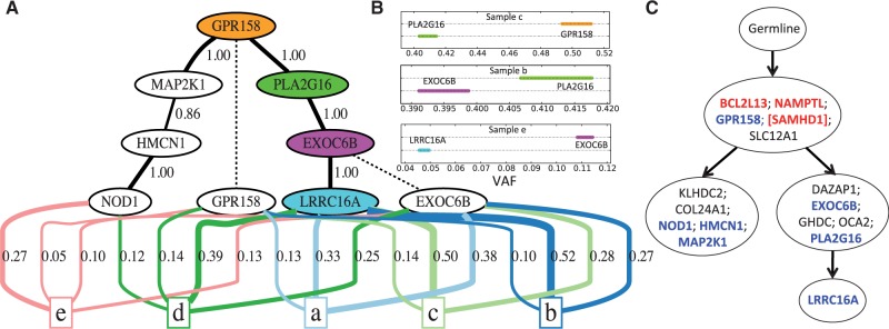
Analysis of CLL patient 077 shows AncesTree’s ability to infer successive clonal expansions. (A) The clonal tree output by AncesTree is indicated by the black solid edges whose weights correspond to the posterior probability of the ancestral relationship. Dashed edges are used to indicate ancestral clones which exist at the time of sequencing. The blocks labeled ‘a’ through ‘e’ each represent a sequenced sample, with colored edges indicating the inferred composition of clones and their fraction in each sample (only edges with usage at least 0.05 are shown). (B) The confidence intervals of VAF for the sample with the weakest ancestral evidence for each of the edges connecting gene GPR158 to LRRC16A. (C) The tree reported by PhyloSub, which is identical to the tree reported by CITUP except for the addition of SAMHD1. Mutations indicated in blue are those present in part A. Mutations indicated in red likely occur in regions affected by copy number aberrations
In addition to the differences in ancestry, the clonal tree output by AncesTree contains only a subset of the mutations, whereas the tree output by PhyloSub contains all mutations. We find that three of the missing mutations (in genes BCL2L13, NAMPTL and SAMHD1) have VAFs that are significantly higher than 0.5. Indeed the confidence interval used by our ILP implementation is strictly larger than 0.5. It is likely that these mutations occur in regions affected by copy number aberrations, thus violating the assumptions of our model. We examined the approximate ancestry graph for this sample (Supplementary Fig. A7) to determine why other mutations were missing from the tree output by AncesTree. We find that mutations in SLC12A1 and GPR158 only have incoming arcs from the three genes listed above whose VAFs exceed 0.5. Thus, there is no subtree of the ancestry graph that contains both SLC12A1 and GPR158. The other missing mutations (KLHDC2, COL24A1, DAZAP1, GHDC and OCA2) are all descendants of SLC12A in the ancestry graph. Of these missing mutations, all except for GHDC are also descendants of GPR158, but each violates the sum condition if added to the tree output by AncesTree.
3.4 Heterogeneity within samples
As AncesTree directly computes the usage matrix U, we obtain estimates of the amount of mixing, or intra-tumor heterogeneity, of clones within each analyzed sample. Specifically, for a given sample, the number of clones that are inferred to be mixed in a sample is the number of non-zero entries in the corresponding row of U. For each tumor, we compute its mixing proportion to be the fraction of entries in U that are non-zero (see Supplementary Table A1). Using the deep sequencing data, we find that the CLL tumors have on average a mixing proportion of 1.0. This is much higher than the renal and lung tumors which have on average mixing proportions of 0.22 and 0.5, respectively. The higher mixing proportions for CLL are consistent with it being a liquid tumor, where mixing between clones is likely to be more common than in solid tumors.
We further analyzed one renal tumor, EV006, for which we obtained a relatively low mixing proportion of 0.21 (Fig. 6). Samples R6 and R7 from this tumor were found to be the mixture of two and three distinct clones, respectively, that do not appear in other samples. This shows that AncesTree can infer the composition of individual samples containing clones distinct from all other samples. The remaining samples in this tumor all include a clone that appears in at least one other sample. Notably, the two lymph node samples, LN1a and LN1b, are inferred to be mixtures of the same two clones. The only difference between these two samples appears to be that LN1b contains a higher admixture with normal cells (0.45) than LN1a (< 0.01), and indeed the two lymph node samples are grouped together in the original analysis of this tumor by Gerlinger et al. (2014).
Fig. 6.

Analysis of renal patient EV006 reveals distinctive sample composition. The clonal tree output by AncesTree. Some sequenced sections (R6, R7) are mixtures of clones appearing only in those sections. In contrast, other sequenced sections (LN1a, LN1b and R3) are mixtures of clones that each appear in more than one section. In particular, both lymph node samples (LN1a and LN1b) are mixtures of the same two clones but in different proportions
4 Discussion
Reconstructing the evolutionary history of a tumor given VAFs measured in multiple sequenced samples for a single tumor is a challenging task. In this work, we formalize this problem as the VAFFP. We derive a combinatorial characterization of the solutions to this problem and prove the problem is NP-complete. We present the AncesTree algorithm for solving an approximate version of the problem which allows errors and demonstrate the advantages of AncesTree relative to existing approaches.
There are a number of avenues for further investigation. First, we have ignored the effect of copy number aberrations on VAFs, meaning that AncesTree may not currently be applicable to some datasets. Second, AncesTree only outputs the single largest rooted subtree of the approximate ancestry graph that satisfies the sum condition. The algorithm may be applied iteratively by removing the clonal tree found at each step from the ancestry graph and re-running, thus returning a forest. However, it is unclear how the trees in this forest relate to each other or if there is an approach for joining them. Third, the theoretical results may be strengthened. For example, as the number m of samples is much smaller than the number n of mutations, it would be interesting to see if the problem is fixed-parameter tractable. Finally, our use of the binomial distribution to model read counts may underestimate the variance; e.g. due to factors such as PCR artifacts. More realistic models of read counts may improve the performance of AncesTree.
Finally, we note that the kidney and lung datasets analyzed here contain multiple sections of a solid tumor obtained at a single time point, whereas the CLL datasets contain samples obtained at different times. Future work will include handling multi-section samples and multi-time-point samples separately to account for time related dependencies.
Funding
This work was supported by a National Science Foundation (NSF) CAREER Award CCF-1053753 and NIH RO1HG005690. B.J.R. was also supported by a Career Award at the Scientific Interface from the Burroughs Wellcome Fund, an Alfred P Sloan Research Fellowship.
Conflict of Interest: none declared.
Supplementary Material
References
- Cook J. (2005) Exact calculation of beta inequalities. Technical report . UT MD Anderson Cancer Center Department of Biostatistics. [Google Scholar]
- Ding L., et al. (2012) Clonal evolution in relapsed acute myeloid leukaemia revealed by whole-genome sequencing. Nature , 481, 506–510. [DOI] [PMC free article] [PubMed] [Google Scholar]
- Gerlinger M., et al. (2012) Intratumor heterogeneity and branched evolution revealed by multiregion sequencing. N. Engl. J. Med. , 366, 883–892. [DOI] [PMC free article] [PubMed] [Google Scholar]
- Gerlinger M., et al. (2014) Genomic architecture and evolution of clear cell renal cell carcinomas defined by multiregion sequencing. Nat. Genet. , 46, 225–233. [DOI] [PMC free article] [PubMed] [Google Scholar]
- Gusfield D. (1991) Efficient algorithms for inferring evolutionary trees. Networks , 21, 19–28. [Google Scholar]
- Gusfield D. (1997) Algorithms on Strings, Trees, and Sequences—Computer Science and Computational Biology . Cambridge University Press, Cambridge, UK. [Google Scholar]
- Hajirasouliha I., Raphael B.J. (2014) Reconstructing mutational history in multiply sampled tumors using perfect phylogeny mixtures. In: Brown D., Morgenstern B. (eds), Algorithms in Bioinformatics—14th International Workshop, WABI 2014, Springer, pp. 354–367. [Google Scholar]
- Hajirasouliha I., et al. (2014) A combinatorial approach for analyzing intra-tumor heterogeneity from high-throughput sequencing data. Bioinformatics , 30, i78–i86. [DOI] [PMC free article] [PubMed] [Google Scholar]
- Jiao W., et al. (2014) Inferring clonal evolution of tumors from single nucleotide somatic mutations. BMC Bioinformatics , 15, 35. [DOI] [PMC free article] [PubMed] [Google Scholar]
- Malikic S., et al. (2015) Clonality inference in multiple tumor samples using phylogeny. Bioinformatics , 31, 1349–1356. [DOI] [PubMed] [Google Scholar]
- Miller C.A., et al. (2014) Sciclone: inferring clonal architecture and tracking the spatial and temporal patterns of tumor evolution. PLoS Comput. Biol. , 10, e1003665. [DOI] [PMC free article] [PubMed] [Google Scholar]
- Navin N.E. (2014) Cancer genomics: one cell at a time. Genome Biol. , 15, 452. [DOI] [PMC free article] [PubMed] [Google Scholar]
- Newburger D.E., et al. (2013) Genome evolution during progression to breast cancer. Genome Res. , 23, 1097–1108. [DOI] [PMC free article] [PubMed] [Google Scholar]
- Nik-Zainal S., et al. (2012) The life history of 21 breast cancers. Cell , 149,994–1007. [DOI] [PMC free article] [PubMed] [Google Scholar]
- Nowell P.C. (1976) The clonal evolution of tumor cell populations. Science , 194, 23–28. [DOI] [PubMed] [Google Scholar]
- Oesper L., et al. (2013) Theta: inferring intra-tumor heterogeneity from high-throughput DNA sequencing data. Genome Biol. , 14, R80. [DOI] [PMC free article] [PubMed] [Google Scholar]
- Oesper L., et al. (2014) Quantifying tumor heterogeneity in whole-genome and whole-exome sequencing data. Bioinformatics , 30, 3532–3540. [DOI] [PMC free article] [PubMed] [Google Scholar]
- Popic V., et al. (2014) Fast and scalable inference of multi-sample cancer lineages. CoRR, abs/1412.8574. [DOI] [PMC free article] [PubMed] [Google Scholar]
- Roth A., et al. (2014) Pyclone: statistical inference of clonal population structure in cancer. Nat. Methods , 11, 396–398. [DOI] [PMC free article] [PubMed] [Google Scholar]
- Schuh A., et al. (2012) Monitoring chronic lymphocytic leukemia progression by whole genome sequencing reveals heterogeneous clonal evolution patterns. Blood , 120, 4191–4196. [DOI] [PubMed] [Google Scholar]
- Shah S.P., et al. (2012) The clonal and mutational evolution spectrum of primary triple-negative breast cancers. Nature , 486, 395–399. [DOI] [PMC free article] [PubMed] [Google Scholar]
- Strino F., et al. (2013) Trap: a tree approach for fingerprinting subclonal tumor composition. Nucleic Acids Res. , 41, e165. [DOI] [PMC free article] [PubMed] [Google Scholar]
- Wang Y., et al. (2014) Clonal evolution in breast cancer revealed by single nucleus genome sequencing. Nature , 512, 155–160. [DOI] [PMC free article] [PubMed] [Google Scholar]
- Wolsey L. (1998) Integer Programming . Wiley-Interscience series in discrete mathematics and optimization. Wiley, New York. [Google Scholar]
- Zare H., et al. (2014) Inferring clonal composition from multiple sections of a breast cancer. PLoS Comput. Biol. , 10, e1003703. [DOI] [PMC free article] [PubMed] [Google Scholar]
- Zhang J., et al. (2014) Intratumor heterogeneity in localized lung adenocarcinomas delineated by multiregion sequencing. Science , 346, 256–259. [DOI] [PMC free article] [PubMed] [Google Scholar]
Associated Data
This section collects any data citations, data availability statements, or supplementary materials included in this article.