Misassembly detection using paired-end sequence reads and optical mapping data

Abstract

Motivation: A crucial problem in genome assembly is the discovery and correction of misassembly errors in draft genomes. We develop a method called misSEQuel that enhances the quality of draft genomes by identifying misassembly errors and their breakpoints using paired-end sequence reads and optical mapping data. Our method also fulfills the critical need for open source computational methods for analyzing optical mapping data. We apply our method to various assemblies of the loblolly pine, Francisella tularensis, rice and budgerigar genomes. We generated and used stimulated optical mapping data for loblolly pine and F.tularensis and used real optical mapping data for rice and budgerigar.

Results: Our results demonstrate that we detect more than 54% of extensively misassembled contigs and more than 60% of locally misassembled contigs in assemblies of F.tularensis and between 31% and 100% of extensively misassembled contigs and between 57% and 73% of locally misassembled contigs in assemblies of loblolly pine. Using the real optical mapping data, we correctly identified 75% of extensively misassembled contigs and 100% of locally misassembled contigs in rice, and 77% of extensively misassembled contigs and 80% of locally misassembled contigs in budgerigar.

Availability and implementation: misSEQuel can be used as a post-processing step in combination with any genome assembler and is freely available at http://www.cs.colostate.edu/seq/.

Contact: muggli@cs.colostate.edu

Supplementary information: Supplementary data are available at Bioinformatics online.

1 Introduction

Comparing genetic variation between and within a species is a fundamental activity in biological research. For example, there is currently a major effort to sequence entire genomes of agriculturally important plant species to identify parts of the genome variable in a given breeding program and, ultimately, create superior plant varieties. Robust genome assembly methods are imperative to these large sequencing initiatives and other scientific projects (Haussler et al. 2008; Ossowski et al. 2008; Robinson et al. 2011; Turnbaugh et al. 2007) because scientific analyses frequently use those genomes to determine genetic variation and associated biological traits.

At present, the majority of assembly programs are based on the Eulerian assembly paradigm (Idury and Waterman 1995; Pevzner et al. 2001), where a de Bruijn graph is constructed with a vertex v for every $(k-1)$-mer present in a set of reads and an edge $(v,v\prime )$ for every observed k-mer in the reads with $(k-1)$-mer prefix v and $(k-1)$-mer suffix $v\prime$. A contig corresponds to a non-branching path through this graph. We refer the reader to Compeau et al. (2011) for a more thorough explanation of de Bruijn graphs and their use in assembly. SPAdes (Bankevich et al. 2012), IDBA (Peng et al. 2012), Euler-SR (Chaisson and Pevzner 2008), Velvet (Zerbino and Birney 2008), SOAPdenovo (Li et al. 2010), ABySS (Simpson et al. 2009) and ALLPATHS (Butler et al. 2008) all use this paradigm and follow the same general outline: extract k-mers from the reads, construct a de Bruijn graph from the set k-mers, simplify the graph and construct contigs.

One crucial problem that persists in Eulerian assembly (and genome assembly, in general) is the discovery and correction of misassembly errors in draft genomes. We define a misassembly error as an assembled region that contains a significantly large insertion, deletion, inversion, or rearrangement that is the result of decisions made by the assembly program. Identification of misassembly errors is important because true biological variations manifest in similar ways, and thus, these errors can be easily misconstrued as true genetic variation (Salzberg 2005). This can mislead a range of genomic analyses. We note that the exact definition of a misassembly error can vary and adopt the standard definition used by QUAST (Gurevich et al. 2013) and other tools. See Section 3.1 for this exact definition. Once the existence and location of a misassembly are identified, it can be removed by segmenting the contig at that location.

We present a computational method for identifying misassembly errors using a combination of short reads and optical mapping data. Optical mapping is a system developed in 1993 (Schwartz et al. 1993) that can construct ordered, genome-wide, high-resolution restriction maps. The system works as follows (Aston and Schwartz 2006; Dimalanta et al. 2004): an ensemble of DNA molecules adhered to a charged glass plate is elongated by fluid flow. An enzyme is then used to cleave them into fragments at loci where the corresponding recognition sequence occurs. Next, the fragments are highlighted with fluorescent dye and imaged under a microscope. Finally, these images are analyzed to estimate the fragment sizes, producing a molecular map. Since the fragments stay relatively stationary during the aforementioned process, the images capture their relative order and size (Neely et al. 2011). Multiple copies of the genome undergo this process, and a consensus map is formed that consists of an ordered sequence of fragment sizes, each indicating the approximate number of bases between occurrences of the recognition sequence in the genome (Anantharaman and Mishra 2001).

Although optical mapping data have been used for discerning structural variation in the human genome (Teague et al. 2010) and for scaffolding and validating contigs for several large sequencing projects—including those for various prokaryote species (Reslewic et al. 2005; Zhou et al. 2002, 2004), rice (Zhou et al. 2007), maize (Zhou et al. 2009), mouse (Church et al. 2009), goat (Dong et al. 2013), parrot (Howard et al. 2014) and Amborella trichopoda (Chamala et al. 2013)—there are no publicly available tools for using this data for misassembly detection using short read and optical mapping data. In 2014, Mendelowitz and Pop (2014) further this point stating that ‘There is, thus, a critical need for the continued development and public release of software tools for processing optical mapping data, mirroring the tremendous advances made in analytical methods for second- and third-generation sequencing data’.

Our tool, which we call sc>/sc>, predicts which contigs are misassembled and the approximate locations of the errors in the contigs. It takes as input the paired-end sequence read data, contigs, an ensemble of optical maps and the restriction enzymes used to construct the optical maps. misSEQuel first uses the paired-end read data to divide the contigs into two sets: those that are predicted to be correctly assembled and those that are not. Then the set of contigs that are candidates for containing misassembly errors are further divided into misassembled contigs and correctly assembled contigs using optical mapping data. Fundamental to the first step is the concept of a red–black positional de Bruijn graph, which encapsulates recurring artifacts in the alignment of the sequence read data to the contigs and their position in the contig. The red vertices in this graph indicate if a contig is likely to be misassembled and also flag the location where the misassembly error occurs. These locations are called misassembly breakpoints.

In the second stage of misSEQuel where optical mapping data are used, the contigs conjectured to be misassembled are in silico digested with the set of input restriction enzymes and aligned to the optical map using Twin (Muggli et al. 2014). Based on the presence or absence of alignment, a prediction of misassembly is made. The in silico digestion process computationally mimics how each restriction enzyme would cleave the segment of DNA defined by the contig, returning ‘mini-optical maps’ that can be aligned to the optical map for the whole genome. An important aspect of our work is that it highlights the need to use another source of information, which is independent of the sequence data but representative of the same genome, to identify misassembly errors. We show that optical mapping data can be used as this information source.

We give results for the Francisella tularensis, loblolly pine, rice and budgerigar genomes. Each genome was assembled using various de Bruijn graph assemblers, and then misassembly errors were predicted. We present results for both real and simulated optical mapping data; simulated data were generated for the F.tularensis and loblolly pine genomes, and real optical mapping data for the rice and budgerigar genomes. Our results on F.tularensis show that misSEQuel correctly identifies (on average) 86% and 80% of locally and extensively misassembled contigs, respectively. This is a considerable improvement on existing methods, which identified (on average) 26% and 16% of locally and extensively misassembled contigs, respectively, in the same assemblies. The results on the loblolly pine genome assemblies show similar improvement. Out of the 499 extensively and 3 locally misassembled contigs in the SOAPdenovo assembly of rice, misSEQuel correctly identified 374 (75%) and 3 (100%) of them, respectively. Competing methods identified between 25% and 30% of these extensively misassembled contigs, and none of these locally misassembled contigs. Lastly, we downloaded the latest Illumina-454 hybrid assembly of budgerigar that was released by Ganapathy et al. (2014), and predicted misassembly errors using the accompanied Illumina paired-end data and optical mapping data. misSEQuel correctly identified 10 777 of the 13 996 extensively misassembled contigs (77%) and 2350 (out of 2937) locally misassembled contigs (80%). Hence, we tested our method across four different genomes, which all vary in size and GC content.

Our conclusions, based on these experimental results, are that the specificity of misSEQuel significantly increases by incorporating optical mapping data into the prediction of misassembly errors, and the sensitivity of misSEQuel is substantially better in comparison to competing methods that just use paired-end data. Therefore, we show evidence that optical mapping data can be a powerful tool for misassembly identification.

1.1 Related work

Amosvalidate (Phillippy et al. 2008), REAPR (Hunt et al. 2013) and Pilon (Walker et al. 2014) are capable of identifying and correcting misassembly errors. REAPR is designed to use both short insert and long insert paired-end sequencing libraries; however, it can operate with only one of these types of sequencing data. Amosvalidate, which is included as part of the AMOS assembly package (Treangen et al. 2011), was developed specifically for first generation sequencing libraries (Phillippy et al. 2008). iMetAMOS (Koren et al. 2014) is an automated assembly pipeline that provides error correction and validation of the assembly. It packages several open-source tools and provides annotated assemblies that result from an ensemble of tools and assemblers. Currently, it uses REAPR for misassembly error correction. Pilon (Walker et al. 2014) detects a variety (including misassembly) of errors in draft genomes and variant detection. Similar to REAPR, Pilon is specifically designed to use short insert and long insert libraries but unlike REAPR and amosvalidate, it is specifically designed for microbial genomes.

Many optical mapping tools exist and deserve mentioning, including AGORA (Lin et al. 2012), SOMA (Nagarajan et al. 2008) and Twin (Muggli et al. 2014). AGORA (Lin et al. 2012) uses the optical map information to constrain de Bruijn graph construction with the aim of improving the resulting assembly. SOMA (Nagarajan et al. 2008) uses dynamic programming to align in silico-digested contigs to an optical map. Twin (Muggli et al. 2014) is an index-based method for aligning contigs to an optical map. Because of its use of an index data structure, it is capable of aligning in silico-digested contigs orders of magnitude faster than competing methods. Xavier et al. (2014) demonstrated misassembly errors in bacterial genomes can be detected using proprietary software.

Lastly, there are special purpose tools that have some relation to misSEQuel in their algorithmic approach. Numerous assembly tools use a finishing process after assembly, including Hapsembler (Donmez and Brudno 2011), LOCAS (Klein et al. 2011), Meraculous (Chapman et al. 2011) and the ‘assisted assembly’ algorithm (Gnerre et al. 2009). Hapsembler (Donmez and Brudno 2011) is a haplotype-specific genome assembly toolkit that is designed for genomes that are highly polymorphic. RACA (Kim et al. 2013) and SCARPA (Donmez and Brudno 2013) are two scaffolding algorithms that perform paired-end alignment to the contigs as an initial step and, thus, are similar to our algorithm in that respect.

2 Methods

misSEQuel can be broken down into four main steps: recruitment of reads to contigs, construction of the red–black positional de Bruijn graph, misassembly error prediction and misassembly verification using optical mapping data. We explain each of these steps in detail in the following subsections.

2.1 Recruitment of reads and threshold calculation

misSEQuel first aligns reads to contigs to identify regions that contain abnormal read alignments. Collapsed or expanded repeats will present as the read coverage being greater or lower than the expected genome coverage in the region that has been misassembled. Similarly, inversion and rearrangement errors will present as the alignment of the mate-pairs being rearranged. Figure 1 illustrates these concordant and discordant read alignments. More specifically, this step consists of aligning all the (paired-end) reads to all the contigs and then calculating three thresholds, Δ_L, Δ_U and Γ. The range $[{\Delta }_L,{\Delta }_U]$ defines the acceptable read depth, and Γ defines the maximum allowable number of reads whose mate-pair aligns in an inverted orientation. To calculate these thresholds, we consider all alignments of each read as opposed to just the best alignment of each read since misassembly errors frequently occur within repetitive regions where the reads will align to multiple locations. misSEQuel performs this step using BWA (version 0.5.9) in paired-end mode with default parameters (Li and Durbin 2009). Subsequently, after alignment, each contig is treated as a series of consecutive 200-bp regions. These are sampled uniformly at random $\ell$ times, and the mean (µ_d) and the standard deviation (σ_d) of the read depth and the mean (µ_i) and the standard deviation (σ_i) of the number of alignments where a discordant mate-pair orientation is witnessed are calculated from these sampled regions. Δ_L is set to the maximum of $\{0,{\mu }_d-3{\sigma }_d\}$, Δ_U is set to ${\mu }_d+3{\sigma }_d$ and Γ is set to ${\mu }_i+3{\sigma }_i$. The default for $\ell$ is $\frac{1}{20}$th of the contig length, and this parameter can be changed in the input to misSEQuel.

Fig. 2.

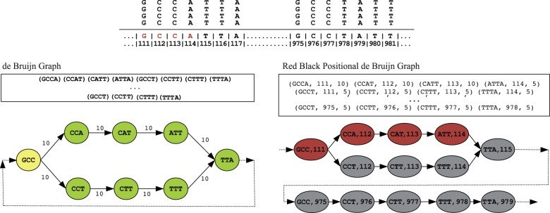
An example illustrating the red black positional de Bruijn graph ($k=4,\Delta =1$), the positional de Bruijn graph and the de Bruijn graph on a set of aligned reads, with their corresponding sets of k-mers and positional k-mers. There exists a region in the genome that extremely high coverage, which would suggest a possible misassembly error. Namely, the positional k-mers (GCCA, 111), (CCAT, 112) and (CATT, 113) have multiplicity 10, whereas all other positional k-mers have multiplicity 5. In the de Bruijn graph where the position is not taken into account, all k-mers have multiplicity of 10 and there is no evidence of a misassembled region. We note that in this example no vertex gluing operations occur but in more complex instances, vertex gluing will occur when equal k-mers align at adjacent positions

Fig. 1.

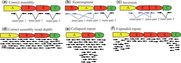
An illustration about the systematic alterations that occur with rearrangements, inversions, collapsed repeats and expanded repeats. (a) Proper read alignment where mate-pair reads have the correct orientation and distance from each other. A rearrangement or inversion will present itself by the orientation of the reads being incorrect and/or the distance of the mate-pairs being significantly smaller or significantly larger than the expected insert size. This is shown in (b) and (c), respectively. (d) The proper read depth, which is uniform across the genome. (e) A collapsed repeat, which results in the read depth being greater than expected. (f) A expanded repeat, which results in the read depth being lower than expected

2.2 Construction of the red–black positional de Bruijn graph

After threshold calculation, the red–black positional de Bruijn graph is constructed. For clarity, we begin by describing the positional de Bruijn graph, given by Ronen et al. (2012) and then define the red–black positional de Bruijn graph. Although the edges in the traditional de Bruijn graph correspond to k-mers, the edges in the positional de Bruijn graph correspond to k-mers and their inferred positions on the contigs (positional k-mers). Hence, the positional de Bruijn graph $G_{k,\Phi }$ is defined for a multiset of positional k-mers and parameter $\Phi$ and is constructed in a similar manner to the traditional de Bruijn graph using an A-Bruijn graph framework from (Pevzner et al. 2004). Given a k-mer s_k, let $\mathrm{prefix}(s_k)$ be the first $k-1$ nucleotides of s_k, and $\mathrm{suffix}(s_k)$ be the last $k-1$ nucleotides of s_k. Each positional k-mer $(s_k,p)$ in the input multiset corresponds to a directed edge in the graph between two positional $(k-1)$-mers, $(\mathrm{prefix}(s_k),p)$ and $(\mathrm{suffix}(s_k),p+1)$. After all edges are formed, the graph undergoes a gluing operation. A pair of positional $(k-1)$-mers, $(s_{k-1},p)$ and $(s_{k-1}\prime ,p\prime )$, are glued together into a single vertex if $s_{k-1}=s_{k-1}\prime$ and $p\in [p\prime -\Phi ,p\prime +\Phi ]$. Two positional $(k-1)$-mers are glued together if their sequences are the same and their positions are within $\Phi$ from each other. We refer to the multiplicity of a positional $(k-1)$-mer $(s_{k-1},p)$ as the number of occurrences where $s_{k-1}$ clustered at position p.

misSEQuel constructs the red–black positional de Bruijn graph from the alignment of the reads to the contigs. The red–black positional de Bruijn graph contains positional k-mers and is constructed in an identical way as the positional de Bruijn graph with the addition that each vertex ($(k-1)$-mer) has an associated red or black color attributed to it that is defined using Δ_L, Δ_U and Γ. In addition to the multiplicity of each positional $(k-1)$-mer, the number of positional $(k-1)$-mers that originated from a read whose mate-pair did not align in the conventional direction is stored at each vertex. When the multiplicity is less than Δ_L or greater than Δ_U or if the observed frequency of discordant mate-pair orientation is greater than Γ, then the vertex is red; otherwise it is black.

2.3 Misassembly conjecture and breakpoint estimation

A red–black positional de Bruijn graph is constructed for each contig, and misassembly errors in each contig are detected by searching for consecutive red vertices in the corresponding graph. Depth-first search is used for the graph traversal. If there are greater than 50 consecutive red vertices, then the contig is conjectured to be misassembled. The breakpoint in the contig can be determined by recovering the position of the corresponding red vertices (e.g. the positional $(k-1)$-mers). The number of consecutive red vertices needed to consider it misassembled can be changed via a command line parameter in misSEQuel. Our experiments were performed with the default (e.g. 50), which corresponds to a region in the contig that has length $\ge$50 bp. After this stage of the algorithm, we take contigs having regions exceeding that threshold as a set of contigs that are conjectured to be misassembled and their transitions in and out of those regions as breakpoints.

2.4 Misassembly verification

Lastly, we use optical mapping data to verify whether a contig that is conjectured to be misassembled indeed is. Verification is based on the expectation that, after in silico digestion, a correctly assembled contig has a sequence of fragment sizes that is similar to that in the optical map at the corresponding locus in the genome. In other words, an in silico-digested contig should align to some region of the optical map since both are derived from the same region in the genome. Conversely, as misassembled contigs are not faithful reconstructions of any part of the genome, when in silico digested, their sequence of fragments will likewise not have a corresponding locus in the optical map to which it aligns.

Optical maps contain measurement error at each fragment size, so some criteria is needed to decide whether variation in fragment size of an in silico-digested contig and that of an optical map at a particular locus is due to variation in the size of the physical fragments or a consequence of optical measurement error. Because of this ambiguity, and the necessary tolerances to ensure correctly assembled contigs align to the locus in the optical map, misassembled contigs may also align to loci in the optical map, which by coincidence have a fragment sequence similar to the contig within the threshold margin of error. Although there are various sophisticated approaches to determining statistical significance of an alignment, such as by Sarkar et al. (2012), we use a ${\chi }^2$ model discussed by Nagarajan et al. (2008) and take the cumulative density function $\le$0.85 as evidence of alignment, which we found to work well empirically.

In addition, a misassembled contig only fails to align to the optical map if the enzyme recognition sequence, and thus the cleavage sites, exist in the contig in a manner that disrupts a good alignment (e.g. a misassembled contig with an inverted segment may still align if cleavage sites flank the inverted segment). This implies that (i) some enzymes produce optical maps that have greater performance in identifying misassembly errors and (ii) alignment to the optical map is not as strong evidence for correct assembly as non-alignment to the optical map is for misassembly. This leads to the conclusion that an ensemble of optical maps (each made with a different enzyme) has a greater chance at revealing misassembly errors than a single optical map. As acquiring three optical maps for one genome is reasonably accessible for many sequencing projects, the process of in silico digestion and alignment is repeated for three enzymes. A contig is deemed to be misassembled if it fails to align to any one of the three optical maps. The alignment is performed using Twin (Muggli et al. 2014) (with default parameters) and then these results are filtered according to the ${\chi }^2$ model mentioned above. For our experiments, optical maps were simulated by in silico digesting reference genomes, adding normally distributed noise with a 150 bp standard deviation and discarding fragments smaller than 700 bp.

3 Analyses

3.1 Datasets using simulated optical mapping data

Our first dataset consisted of approximately 6.9 million paired-end 101 bp reads from the prokaryote genome F.tularensis, generated by Illumina Genome Analyzer (GA) IIx platform. It was obtained from the NCBI Short Read Archive [accession number (SRA:SRR063416)]. The reference genome was also downloaded from the NCBI website [Reference genome (RefSeq:NC_006570.2)]. The F.tularensis genome is 1 892 775 bp in length with a GC content of 32%. As a measure of quality assurance, we aligned the reads to the F.tularensis genome using BWA (version 0.5.9) (Li and Durbin 2009) with default parameters. We call a read mapped if BWA outputs an alignment for it and unmapped otherwise. Analysis of the alignments revealed that 97% of the reads mapped to the reference genome representing an average depth of approximately $367\times$.

Our second dataset consisted of approximately 31.3 million paired-end 100 bp reads from the loblolly pine (Pinus taeda) genome (Neale et al. 2014), which has GC contact of 38%. We downloaded the reference genome from the pine genome website (http://pinegenome.org/pinerefseq) and simulated reads from the largest five hundred scaffolds from the reference using ART (Huang et al. 2012) (‘art illumina’). ART was ran with parameters that simulated 100 bp paired end reads with 200 bp insert size and 50x coverage. The data for this experiment are available on the misSEQuel website. We simulated an optical map using the reference genome for F.tularensis and loblolly pine since there is no publicly available one for these genomes.

We assembled both sets of reads with a wide variety of state-of-the-art assemblers. The versions used were those that were publicly available before or on September 1, 2014: SPAdes (version 3.1) (Bankevich et al. 2012); Velvet (version 1.2.10) (Zerbino and Birney 2008); SOAPdenovo (version 2.04) (Li et al. 2010); ABySS (version 1.5.2) (Simpson et al. 2009) and IDBA-UD (version 1.1.1) (Peng et al. 2012). SPAdes outputs two assemblies: before repeat resolution and after repeat resolution—we report both. Some of the assemblers emitted both contigs and scaffolds. We considered contigs only but note that all scaffolds had a greater number of misassembly errors. We emphasize that our purpose here is not to compare the various assemblers, but instead it is to demonstrate that all assemblers produce misassembly errors, which are in need of consideration and correction.

We used QUAST (Gurevich et al. 2013) in default mode to evaluate the assemblies. Hence, our experiments use the published reference genomes as being ground truth and use the published references to identify misassembly errors in the other assemblies through QUAST. We note that this is imperfect since the reference genomes are likely not error-free. QUAST defines misassembly error as being extensive or local. An extensively misassembled contig is defined as one that satisfies one following conditions: (i) the left flanking sequence aligns over 1 kb away from the right flanking sequence on the reference; (ii) flanking sequences overlap on more than 1 kb and (iii) flanking sequences align to different strands or different chromosomes, whereas a local misassembled contig is one that satisfies the following conditions: (i) two or more distinct alignments cover the breakpoint; (ii) the gap between left and right flanking sequences is less than 1 kb and the left and right flanking sequences both are on the same strand of the same chromosome of the reference genome. We made a minor alteration to QUAST to output which contigs contain local misassembly errors. A contig can contain both extensive and local misassembly errors. Any correctly assembled contig is one that does not contain either type of error.

3.1.1 Detection of misassembly errors in F.tularensis

Table 1 gives the assembly statistics corresponding to this experiment. Comparable assembly results on this data were reported by Ilie et al. (2014), though in some cases we used more recent software releases (e.g. for SPAdes). Note that the number of locally misassembled contigs and the number of extensively misassembled contigs is not disjoint. A contig can be locally and extensively misassembled. Thus, Table 1 gives the number of contigs having at least one extensive misassembly error and the number of contigs having at least one local misassembly error.

Table 1.

The performance comparison between major assembly tools on the F.tularensis dataset, which has a genome length of 1 892 775 bp and 6 907 220 number of 101 bp reads, using QUAST in default mode (Gurevich et al. 2013)

Assembler	No. contigs (no. unaligned)	N50	Largest (bp)	Total (bp)	MA	local MA	MA (bp)	GF (%)
Velvet	358 (3 + 35 part)	7377	39 381	1 762 202	11	36	84 965	92.09
SOAPdenovo	307 (3 + 31 part)	8767	39 989	2 018 158	10	35	96 258	92.05
ABySS	96 (1 part)	27 975	88 275	1 875 628	64	32	1 330 684	95.87
SPAdes (−rr)	102 (2 + 11 part)	25 148	87 449	1 788 634	11	30	258 309	92.81
SPAdes (+rr)	100 (2 + 17 part)	26 876	87 891	1 797 197	23	31	497 356	93.75
IDBA	109 (1 + 10 part)	23 223	87 437	1 768 958	10	31	221 087	92.64

All statistics are based on contigs no shorter than 500 bp. N50 is defined as the length for which the collection of all contigs of that length or longer contains at least half of the sum of the lengths of all contigs and for which the collection of all contigs of that length or shorter also contains at least half of the sum of the lengths of all contigs. The no. unaligned is the number of contigs that did not align to the reference genome, or they were only partially aligned (part). Total is sum of the length of all contigs. MA is the number of (extensively) misassembled contigs. Local MA is the total number of contigs that had local misassemblies. MA (bp) is the total length of the MA contigs. GF is the genome fraction percentage, which is the fraction of genome bases that are covered by the assembly. −rr and ++rr denotes before and after repeat resolution, respectively.

Table 2 shows the results for (i) misSEQuel with paired-end data only; (ii) misSEQuel with optical mapping data only and (iii) misSEQuel with both optical mapping and paired-end data to demonstrate the benefit of combining both types of data. As demonstrated by these results, using short paired-end data alone produced a high false-positive rate (FPR) due to ambiguous read mapping in locations that contain repetitive regions. This is an inherent shortcoming of short paired-end data and demonstrates that to decrease the FPR, another source of information must be used in combination. Optical mapping data have a much lower FPR and when used in combination with paired-end data, produces optimal results. The lowest FPR was witnessed when both optical mapping and paired-end data were used. In some cases, the reduction in the FPR was dramatic: from 87% (ABySS, paired-end data) to 13% (ABySS, paired-end and optical mapping data). The true-positive rate (TPR) of locally misassembled contigs was between 77% and 100% when both paired-end and optical mapping data were used. Lastly, TPR of extensively misassembled contigs was between 55% and 100% when both paired-end and optical mapping data were used.

Table 2.

The performance comparison of our method on the F.tularensis dataset

Correction method	Assembler	MA TPR	local MA TPR	FPR
misSEQuel (paired-end data only)	Velvet	100% (11/11)	100% (36/36)	58% (180/312)
	SOAPdenovo	100% (10/10)	100% (35/35)	63% (165/263)
	ABySS	100% (64/64)	100% (32/32)	87% (20/23)
	SPAdes (−rr)	100% (11/11)	100% (30/30)	83% (52/63)
	SPAdes (++rr)	100% (23/23)	100% (31/31)	86% (49/57)
	IDBA	100% (10/10)	100% (31/31)	38% (57/149)
misSEQuel (optical mapping data only)	Velvet	55% (6/11)	69% (25/36)	24% (76/312)
	SOAPdenovo	80% (8/10)	63% (22/35)	29% (77/263)
	ABySS	69% (44/64)	88% (28/32)	13% (3/23)
	SPAdes (−rr)	91% (10/11)	87% (26/30)	21% (13/63)
	SPAdes (++rr)	87% (20/23)	81% (25/31)	16% (9/57)
	IDBA	90% (9/10)	77% (24/31)	10% (15/149)
misSEQuel (paired-end and optical mapping data)	Velvet	55% (6/11)	100% (36/36)	22% (68/312)
	SOAPdenovo	80% (8/10)	84% (21/35)	20% (53/263)
	ABySS	69% (44/64)	88% (28/32)	13% (3/23)
	SPAdes (−rr)	91% (10/11)	87% (26/30)	19% (12/63)
	SPAdes (++rr)	97% (20/23)	81% (25/31)	16% (9/57)
	IDBA	90% (9/10)	77% (24/31)	9% (14/149)
REAPR	Velvet	55% (6/11)	11% (4/36)	< 1% (2/312)
	SOAPdenovo	20% (2/10)	14% (5/35)	2% (6/263)
	ABySS	13% (8/64)	13% (4/32)	4% (1/23)
	SPAdes (−rr)	27% (3/11)	27% (8/30)	5% (3/63)
	SPAdes (++rr)	0% (0/23)	19% (6/31)	11% (6/57)
	IDBA	40% (4/10)	13% (4/31)	4% (6/149)
Pilon	Velvet	27% (3/11)	3% (1/36)	< 1% (3/312)
	SOAPdenovo	10% (1/10)	9% (3/35)	2% (5/263)
	ABySS	3% (2/64)	6% (2/32)	4% (3/23)
	SPAdes (−rr)	0% (0/11)	3% (1/30)	5% (5/63)
	SPAdes (++rr)	0% (0/23)	10% (3/31)	12% (7/57)
	IDBA	0% (0/10)	10% (3/31)	4% (5/149)

The TPR in this context is a contig that is misassembled and is predicted to be so. The FPR is a correctly assembled contig that was predicted to be misassembled. The TPR and FPR are given as percentages with the raw values given in brackets. Bold values emphasize the benefit of using both data sources.

In our experiments, we iterate through combinations of three enzymes from the REBASE enzyme database (Roberts et al. 2010) and use the set of enzymes that performed best. Our results demonstrate that with a good enzyme choice over half of all extensively misassembled contigs and over 75% of locally misassembled contigs can be identified with only a 9–22% false discovery rate.

3.1.2 Detection of misassembly errors in loblolly pine

Table 3 gives the assembly statistics corresponding to this experiment. The results for the loblolly pine are listed in Table 4. Both Velvet and SOAPdenovo produced zero misassembled contigs on this dataset, so we do not include them in Table 4. misSEQuel correctly identifies between 31% and 100% of extensively misassembled contigs and between 57% and 73% of locally misassembled contigs. The FPR was between 0.6% and 43%. Although REAPR has a lower FPR (between 3% and 11%), it is only capable of identifying a small number of extensively misassembled contigs (between 2% and 14%) and a small number of locally misassembled contigs (between 2% and 27%). Similar to the results of F.tularensis, Pilon had a lower FPR but also lower TPRs than REAPR. This is unsurprising since ‘it is optimized to use both fragment (or small) and long (or large) insert libraries’ and was created for microbial genomes (Walker et al. 2014).

Table 3.

The performance comparison between major assembly tools on Loblolly pine genome dataset (62 647 324 bp, 31.3 million reads, 100 bp) using QUAST in default mode (Gurevich et al. 2013)

Assembler	No. contigs (no. unaligned)	N50	Largest (bp)	Total (bp)	MA	local MA	MA (bp)	GF (%)
Velvet	13 327 (0)	1740	10 823	51 851 131	0	0	0	62.21
SOAPdenovo	16 126 (0 + 1 part)	7950	63 004	57 205 817	0	0	0	90.01
ABySS	4586 (16 + 89 part)	37 089	201 382	63 349 408	127	715	1 391 565	98.17
SPAdes (−rr)	20 671 (4 + 10 part)	4809	44 993	45 079 764	7	11	65 079	81.30
SPAdes (+rr)	8607 (7 + 102 part)	16 957	108 442	59 730 939	299	57	3 734 609	94.57
IDBA	22 409 (3 + 31 part)	3990	40 213	49 765 854	61	200	292 769	79.03

Table 4.

The performance comparison of our method on the loblolly pine dataset

Correction method	Assembler	MA TPR	local MA TPR	FPR
misSEQuel	ABySS	31% (40/127)	57% (405/715)	43% (1604/3754)
	SPAdes (−rr)	100% (7/7)	73% (8/11)	<1% (135/20 653)
	SPAdes (+rr)	67% (199/299)	67% (38/57)	38% (3117/8254)
	IDBA	52% (32/61)	73% (145/200)	19% (4258/22 150)
REAPR	ABySS	7% (9/127)	2% (12/715)	3% (112/3754)
	SPAdes (−rr)	14% (1/7)	27% (3/11)	6% (1323/20 653)
	SPAdes (+rr)	7% (21/299)	5% (3/57)	5% (424/8254)
	IDBA	2% (1/61)	6% (12/200)	11% (2354/22 150)
Pilon	ABySS	7% (8/127)	2% (11/715)	2% (70/3754)
	SPAdes (−rr)	14% (1/7)	18% (2/11)	4% (923/20 653)
	SPAdes (+rr)	5% (16/299)	5% (3/57)	5% (388/8254)
	IDBA	2% (1/61)	5% (12/200)	8% (1823/22 150)

Again, a true positive in this context is a contig that is misassembled and is predicted to be so. A false positive is a correctly assembled contig that was predicted to be misassembled. Bold values highlight MISSEQUEL results.

Again, the restriction enzymes used in our experiments were chosen to be optimal by considering the set of all possible enzymes in the aforementioned database. Nonetheless, we note that if the enzyme combination was chosen at random, then the expected FPR and TPR would decrease by a small fraction for majority of the assemblies considered. The Supplementary Material shows prototypical ROC curves and heat-maps illustrating the density of enzyme combinations at various detection rates.

3.2 Datasets using real optical mapping data

We evaluated the performance of misSEQuel on rice and budgerigar. These genomes were chosen because they have available sequence and optical mapping data, are diverse in size and have undergone a significant level of verification. Rice and budgerigar have genome sizes of 430 Mb and 1.58 Gbp, respectively (Kawahara et al. 2013; Tiersch and Wachtel 1991). The size of budgerigar is only predicted (Tiersch and Wachtel 1991). The validated genomic regions will allow us to use QUAST to determine FPR and TPR, as in Subsection 3.1.

3.2.1 Performance on rice genome

The sequence dataset consists of approximately 134 million 76-bp paired-end reads for rice from the japonica cultivar Nipponbare, generated by Illumina, Inc. on the Genome Analyzer (GA) IIx platform (Kawahara et al. 2013). These reads were obtained from the NCBI Short Read Archive (accession SRX032913). The optical map for this same cultivar of rice was constructed by Zhou et al. (2007) using SwaI as the restriction enzyme. This optical map was assembled from single molecule restriction maps into 14 optical map contigs, labeled as 12 chromosomes, with chromosome labels 6 and 11 both containing two optical map contigs. Both the sequence and optical mapping data were generated as part of a larger project that produced a ‘revised, error-corrected, and validated assembly of the Nipponbare cultivar of rice’ (Kawahara et al. 2013). This reference genome, termed Os-Nipponbare-Reference-IRGSP-1.0 is publicly available on the Rice Annotation Project (http://rice.plantbiology.msu.edu/annotation_pseudo_current.shtml)

The paired-end data were assembled using SOAPdenovo using default parameters. This assembly consists of 11 440 contigs larger than 500 bp, cove 81.3% of the reference genome (22 317 126 in size, 43.7% GC content). It has an N50 statistic of 1 680 499 extensively misassembled contigs and 3 locally misassembled contigs. We ran misSEQuel with default parameters and the SOAPdenovo assembly, optical map and paired-end data as input. Similarly, we ran REAPR with default parameters, and the SOAPdenovo assembly, and paired-end data as input. Out of the 499 extensively misassembled contigs, misSEQuel identified 374 of them (75%), whereas REAPR identified 30 (6%) and Pilon identified 25 (5%). Out of the three locally misassembled contigs, misSEQuel identified all three, but REAPR and Pilon identified none. Lastly, misSEQuel deemed that 821 of the correctly assembled contigs were misassembled (<1% FPR), whereas REAPR and Pilon deemed that 800 and 522 were deemed misassembled (<1% FPR), respectively. We further note that both misSEQuel and REAPR agreed on 472 of these correctly assembled contigs; i.e. both REAPR and misSEQuel predicted that 472 correctly assembled contigs are misassembled. This could suggest that a broadened definition of misassembly by QUAST would also deem these contigs to be misassembled.

3.2.2 Misassembly errors in the draft genome of budgerigar

A concerted effort has been in understanding the biodiversity of many bird species (Jarvis et al. 2014)—including the budgerigar genome—and thus, a significant amount of data have been generated for budgerigar. Pacific Biosciences (PacBio) data, short read Illumina data, 454 and optical mapping data have been generated and used for the assembly of this genome. The sequence and optical map data for the budgerigar genome were generated for the Assemblathon 2 project of Bradnam et al. (2013). Budgerigar has a GC content of approximately 43.8% (Jarvis et al. 2014) and contains GC-rich ($\ge$ 75%) regions (Howard et al. 2014). Sequence data consist of a combination of Roche 454, Illumina and PacBio reads, providing 16×, 285× and 10× coverage, respectively, of the genome. All sequence reads are available at the NCBI Short Read Archive (accession ERP002324). For our analysis, we consider the assembly generated using CABOG (Miller et al. 2008), which was completed by the CBCB team (Koren and Phillippy) as part of Assemblathon 2 (Bradnam et al. 2013). The optical mapping data were created by Zhou, Goldstein, Place, Schwartz and Bechner using the SwaI restriction enzyme and consists of 92 separate pieces.

Ganapathy et al.(2014) released three hybrid assemblies; namely, (i) budgerigar 454-Illumina hybrid v6.3 using the CABOG (Miller et al. 2008) assembler; (ii) budgerigar PacBio corrected reads (PBcR) hybrid using the CABOG assembler and (iii) budgerigar Illumina-454 hybrid using the SOAPdenovo (version 2.04) (Li et al. 2010) assembler. We downloaded the PBcR assembly (ii), the Illumina-454 hybrid assembly (iii), in addition to the optical mapping data and pair-end data. The Illumina-454 assembly has 212 203 contigs (54 829 contigs $\ge$ 500 bp), N50 of 51 034 and largest contig of 500 974 (Howard et al. 2014). The PBcR assembly has 77 556 contigs, average, N50 of 102 885 and largest contig of 849 044 (Howard et al. 2014). We ran QUAST to evaluate the Illumina-454 hybrid assembly (all contigs $\ge$ 500 bp), using the PBcR assembly as the reference genome. It reported 13 996 extensively misassembled contigs and 2937 locally misassembled contigs. Thus, there are 39 394 contigs that contain no misassembly error. We ran misSEQuel on the Illumina-454 hybrid assembly on this using the paired-end and optical mapping. misSEQuel correctly identified 10 777 (out of 13 996) extensively misassembled contigs (77% MA TPR) and 2350 (out of 2937) locally misassembled contigs (80% local MA TPR); however, it incorrectly identified 4023 (out of the 39 394) as being misassembled (10%).

3.3 Practical considerations: memory and time

We evaluated the memory and time requirements of misSEQuel. Since misSEQuel is a multi-threaded application, its wall-clock time depends on the computing resources available to the user. misSEQuel required a maximum of 8 threads, 16 GB and 1.5 h on all assemblies of F.tularensis and a maximum of 20 GB and 2.5 h to complete on all assemblies of loblolly pine. Most genome assemblers require an incomparably greater amount of time and memory and thus, from a practical perspective, the requirements of misSEQuel are not a significant increase. The difference in the resource requirements of misSEQuel in comparison to modern assemblers is since it operates contig-wise rather than genome-wise and therefore, only deals with a significantly smaller portion of the data at a single time. We conclude by mentioning that misSEQuel is not optimized for memory and time and both could be further reduced but reimplementing the red–black positional de Bruijn graph using memory- and time-succinct data structures.

4 Discussion and conclusions

This article describes the first non-proprietary computational method for identifying misassembly errors using short read sequence data and optical mapping data. Our results demonstrate (i) a substantial number of misassembly errors can be identified in draft genomes of prokaryote and eukaryote species; (ii) our method works on genomes that vary by GC-content and size; (iii) it can be used in combination with any assembler and thus, making it a viable post-processing step for any assembly and (iv) addresses the need for methods to analyze optical mapping data.

One of our main contributions is the demonstration that optical mapping can have significant benefit for misassembly error detection. A high FPR will result using paired-end data alone because of ambiguous read mapping. Furthermore, superior results were always witnessed using paired-end data and optical mapping data. In some cases, the improvement of using both datasets over a single dataset was substantial. For example, the Velvet assembly of F.tularensis had 312 correctly assembled contigs; 76 of these 312 were deemed to be misassembled when misSEQuel was ran with optical mapping data alone, whereas this improved to 68 out of 312 when both paired-end and optical mapping data were used. Similarly, when misSEQuel was ran on this same assembly, 69% (25/36) of locally misassembled contigs were identified, whereas this improved to 100% (36/36) when both datasets were used.

Lastly, we point out two areas that warrant future work. One area that merits investigation is to develop methods that will distinguish between structural variation heterozygosity and paralogous variation and misassembly errors. misSEQuel is not able to detect the difference between structural variation and misassembly errors—and in fact, the high FPR might be due to this type of variation—however, methods that do so could be very valuable for finishing draft genomes. Lastly, we conclude by suggesting that efficient algorithmic selection of enzymes that will yield such informative optical maps in a de novo scenario is an area for interesting and important future work.

References

- Anantharaman T.S., Mishra B. (2001) False positives in genomic map assembly and sequence validation. In: Proceedings of the First International Workshop on Algorithms in Bioinformatics, WABI ’01, London, UK: Springer, pp. 27–40. [Google Scholar]
- Aston C., Schwartz D. (2006) Optical mapping in genomic analysis. In: Meyers R.A., et al. (eds) Encyclopedia of Analytical Chemistry. Wiley, Hoboken, NJ, pp. 5105–5121. [Google Scholar]
- Bankevich A., et al. (2012) SPAdes: a new genome assembly algorithm and its applications to single-cell sequencing. J. Comput. Biol., 19, 455–477. [DOI] [PMC free article] [PubMed] [Google Scholar]
- Bradnam K., et al. (2013) Assemblathon 2: evaluating de novo methods of genome assembly in three vertebrate species. GigaScience, 2, 1–31. [DOI] [PMC free article] [PubMed] [Google Scholar]
- Butler J., et al. (2008) ALLPATHS: de novo assembly of whole-genome shotgun microreads. Genome Res., 18, 810–820. [DOI] [PMC free article] [PubMed] [Google Scholar]
- Chaisson M., Pevzner P. (2008) Short read fragment assembly of bacterial genomes. Genome Res., 18, 324–330. [DOI] [PMC free article] [PubMed] [Google Scholar]
- Chamala S., et al. (2013) Assembly and validation of the genome of the nonmodel basal angiosperm Amborella. Science, 342, 1516–1517. [DOI] [PubMed] [Google Scholar]
- Chapman J., et al. (2011) Meraculous: de novo genome assembly with short paired-end reads. PLoS One, 6, e23501. [DOI] [PMC free article] [PubMed] [Google Scholar]
- Church D.M., et al. (2009) Lineage-specific biology revealed by a finished genome assembly of the mouse. PLoS Biol., 7, e1000112. [DOI] [PMC free article] [PubMed] [Google Scholar]
- Compeau P., et al. (2011) How to apply de Bruijn graphs to genome assembly. Nat. Biotechnol., 29, 987–991. [DOI] [PMC free article] [PubMed] [Google Scholar]
- Dimalanta E., et al. (2004) Microfluidic system for large DNA molecule arrays. Anal. Chem., 76, 5293–5301. [DOI] [PubMed] [Google Scholar]
- Dong Y., et al. (2013) Sequencing and automated whole-genome optical mapping of the genome of a domestic goat. Nat. Biotechnol., 31, 136–141. [DOI] [PubMed] [Google Scholar]
- Donmez N., Brudno M. (2011) Hapsembler: an assembler for highly polymorphic genomes. In: Proceedings of RECOMB, pp. 38–52. [Google Scholar]
- Donmez N., Brudno M. (2013) SCARPA: scaffolding reads with practical algorithms. Bioinformatics, 29, 428–434. [DOI] [PubMed] [Google Scholar]
- Ganapathy G., et al. (2014) De novo high-coverage sequencing and annotated assemblies of the budgerigar genome. GigaScience, 3, 11. [DOI] [PMC free article] [PubMed] [Google Scholar]
- Gnerre S., et al. (2009) Assisted assembly: how to improve a de novo genome assembly by using related species. Genome Biol., 10, R88. [DOI] [PMC free article] [PubMed] [Google Scholar]
- Gurevich A., et al. (2013) QUAST: quality assessment tool for genome assemblies. Bioinformatics, 29, 1072–1075. [DOI] [PMC free article] [PubMed] [Google Scholar]
- Haussler D., et al. (2008) Genome 10K: a proposal to obtain whole-genome sequence for 10,000 vertebrate species. J. Hered., 100, 659–674. [DOI] [PMC free article] [PubMed] [Google Scholar]
- Huang W., et al. (2012) ART: a next-generation sequencing read simulator. Bioinformatics, 28, 593–594. [DOI] [PMC free article] [PubMed] [Google Scholar]
- Hunt M., et al. (2013) REAPR: a universal tool for genome assembly evaluation. Genome Biol., 14, R47. [DOI] [PMC free article] [PubMed] [Google Scholar]
- Idury R., Waterman M. (1995) A new algorithm for DNA sequence assembly. J. Comput. Biol., 2, 291–306. [DOI] [PubMed] [Google Scholar]
- Ilie L., et al. (2014) SAGE: string-overlap assembly of genomes. BMC Bioinformatics, 15, 302. [DOI] [PMC free article] [PubMed] [Google Scholar]
- Jarvis E., et al. (2014) Whole-genome analyses resolve early branches in the tree of life of modern birds. Science, 346, 1320–1331. [DOI] [PMC free article] [PubMed] [Google Scholar]
- Kawahara Y., et al. (2013) Improvement of the Oryza sativa nipponbare reference genome using next generation sequence and optical map data. Rice, 6, 1–10. [DOI] [PMC free article] [PubMed] [Google Scholar]
- Kim J., et al. (2013) Reference-assisted chromosome assembly. Proc. Natl. Acad. Sci. USA, 110, 1785–1790. [DOI] [PMC free article] [PubMed] [Google Scholar]
- Klein J., et al. (2011) LOCAS–a low coverage assembly tool for resequencing projects. PloS One, 6, e23455. [DOI] [PMC free article] [PubMed] [Google Scholar]
- Koren S., et al. (2014) Automated ensemble assembly and validation of microbial genomes. BMC Bioinformatics, 15, 126. [DOI] [PMC free article] [PubMed] [Google Scholar]
- Li H., Durbin R. (2009) Fast and accurate short read alignment with Burrows–Wheeler transform. Bioinformatics, 25, 1754–1760. [DOI] [PMC free article] [PubMed] [Google Scholar]
- Li R., et al. (2010) De novo assembly of human genomes with massively parallel short read sequencing. Genome Res., 20, 265–272. [DOI] [PMC free article] [PubMed] [Google Scholar]
- Lin H., et al. (2012) AGORA: assembly guided by optical restriction alignment. BMC Bioinformatics, 12, 189. [DOI] [PMC free article] [PubMed] [Google Scholar]
- Mendelowitz L., Pop M. (2014) Computational methods for optical mapping. GigaScience, 3, 33. [DOI] [PMC free article] [PubMed] [Google Scholar]
- Miller J., et al. (2008) Aggressive assembly of pyrosequencing reads with mates. Bioinformatics, 24, 2818–2824. [DOI] [PMC free article] [PubMed] [Google Scholar]
- Muggli M., et al. (2014) Efficient indexed alignment of contigs to optical maps. In: Proceedings of WABI, pp. 68–81. [Google Scholar]
- Nagarajan N., et al. (2008) Scaffolding and validation of bacterial genome assemblies using optical restriction maps. Bioinformatics, 24, 1229–1235. [DOI] [PMC free article] [PubMed] [Google Scholar]
- Neale D., et al. (2014) Decoding the massive genome of loblolly pine using haploid DNA and novel assembly strategies. Genome Biol., 15, R59. [DOI] [PMC free article] [PubMed] [Google Scholar]
- Neely R.K., et al. (2011) Optical mapping of DNA: single-molecule-based methods for mapping genome. Biopolymers, 95, 298–311. [DOI] [PubMed] [Google Scholar]
- Ossowski S., et al. (2008) Sequencing of natural strains of Arabidopsis thaliana with short reads. Genome Res., 18, 2024–2033. [DOI] [PMC free article] [PubMed] [Google Scholar]
- Peng Y., et al. (2012) IDBA-UD: a de novo assembler for single-cell and metagenomic sequencing data with highly uneven depth. Bioinformatics, 28, 1420–1428. [DOI] [PubMed] [Google Scholar]
- Pevzner P., et al. (2001) An Eulerian path approach to DNA fragment assembly. Proc. Natl. Acad. Sci. USA, 98, 9748–9753. [DOI] [PMC free article] [PubMed] [Google Scholar]
- Pevzner P., et al. (2004) De Novo repeat classification and fragment assembly. Genome Res., 14, 1786–1796. [DOI] [PMC free article] [PubMed] [Google Scholar]
- Phillippy A., et al. (2008) Genome assembly forensics: finding the elusive mis-assembly. Genome Biol., 9, R55. [DOI] [PMC free article] [PubMed] [Google Scholar]
- Reslewic S., et al. (2005) Whole-genome shotgun optical mapping of Rhodospirillum rubrum. Appl. Environ. Microbiol., 71, 5511–5522. [DOI] [PMC free article] [PubMed] [Google Scholar]
- Roberts R., et al. (2010) REBASE–a database for DNA restriction and modification: enzymes, genes and genomes. Nucleic Acids Res., 38, D234–D236. [DOI] [PMC free article] [PubMed] [Google Scholar]
- Robinson G.E., et al. (2011). Creating a buzz about insect genomes. Science, 331, 1386–1386. [DOI] [PubMed] [Google Scholar]
- Ronen R., et al. (2012) SEQuel: improving the accuracy of genome assemblies. Bioinformatics, 28, i188–i196. [DOI] [PMC free article] [PubMed] [Google Scholar]
- Salzberg S. (2005) Beware of mis-assembled genomes. Bioinformatics, 21, 4320–4321. [DOI] [PubMed] [Google Scholar]
- Sarkar D., et al. (2012) Statistical significance of optical map alignments. J. Comput. Biol., 19, 478–492. [DOI] [PMC free article] [PubMed] [Google Scholar]
- Schwartz D., et al. (1993) Ordered restriction maps of Saccharomyces cerevisiae chromosomes constructed by optical mapping. Science, 262, 110–114. [DOI] [PubMed] [Google Scholar]
- Simpson J., et al. (2009) ABySS: a parallel assembler for short read sequence data. Genome Res., 19, 1117–1123. [DOI] [PMC free article] [PubMed] [Google Scholar]
- Teague B., et al. (2010) High-resolution human genome structure by single-molecule analysis. Proc. Natl. Acad. Sci. USA, 107, 10848–10853. [DOI] [PMC free article] [PubMed] [Google Scholar]
- Tiersch T., Wachtel S. (1991) On the evolution of genome size of birds. J. Hered., 5, 363–368. [DOI] [PubMed] [Google Scholar]
- Treangen T.J., et al. (2011) Next Generation Sequence Assembly with AMOS, Vol. 11 Wiley, Hoboken, NJ. [DOI] [PMC free article] [PubMed] [Google Scholar]
- Turnbaugh P.J., et al. (2007) The human microbiome project: exploring the microbial part of ourselves in a changing world. Nature, 449, 804. [DOI] [PMC free article] [PubMed] [Google Scholar]
- Walker B., et al. (2014) Pilon: an integrated tool for comprehensive microbial variant detection and genome assembly improvement. PLoS One, 9, e112963. [DOI] [PMC free article] [PubMed] [Google Scholar]
- Xavier B., et al. (2014) Employing whole genome mapping for optimal de novo assembly of bacterial genomes. BMC Res. Notes, 7, 484. [DOI] [PMC free article] [PubMed] [Google Scholar]
- Zerbino D., Birney E. (2008) Velvet: algorithms for de novo short read assembly using de Bruijn graphs. Genome Res., 18, 821–829. [DOI] [PMC free article] [PubMed] [Google Scholar]
- Zhou S., et al. (2002) A whole-genome shotgun optical map of Yersinia pestis strain KIM. Appl. Environ. Microbiol., 68, 6321–6331. [DOI] [PMC free article] [PubMed] [Google Scholar]
- Zhou S., et al. (2004) Shotgun optical mapping of the entire Leishmania major Friedlin genome. Mol. Biochem. Parasitol., 138, 97–106. [DOI] [PubMed] [Google Scholar]
- Zhou S., et al. (2007) Validation of rice genome sequence by optical mapping. BMC Genomics, 8, 278. [DOI] [PMC free article] [PubMed] [Google Scholar]
- Zhou S., et al. (2009) A single molecule scaffold for the maize genome. PLoS Genet., 5, e1000711. [DOI] [PMC free article] [PubMed] [Google Scholar]
Associated Data
This section collects any data citations, data availability statements, or supplementary materials included in this article.