Abstract
Purpose:
Digital breast tomosynthesis (DBT) is a novel modality with the potential to improve early detection of breast cancer by providing three-dimensional (3D) imaging with a low radiation dose. 3D image reconstruction presents some challenges: cone-beam and flat-panel geometry, and highly incomplete sampling. A promising means to overcome these challenges is statistical iterative reconstruction (IR), since it provides the flexibility of accurate physics modeling and a general description of system geometry. The authors’ goal was to develop techniques for applying statistical IR to tomosynthesis imaging data.
Methods:
These techniques include the following: a physics model with a local voxel-pair based prior with flexible parameters to fine-tune image quality; a precomputed parameter λ in the prior, to remove data dependence and to achieve a uniform resolution property; an effective ray-driven technique to compute the forward and backprojection; and an oversampled, ray-driven method to perform high resolution reconstruction with a practical region-of-interest technique. To assess the performance of these techniques, the authors acquired phantom data on the stationary DBT prototype system. To solve the estimation problem, the authors proposed an optimization-transfer based algorithm framework that potentially allows fewer iterations to achieve an acceptably converged reconstruction.
Results:
IR improved the detectability of low-contrast and small microcalcifications, reduced cross-plane artifacts, improved spatial resolution, and lowered noise in reconstructed images.
Conclusions:
Although the computational load remains a significant challenge for practical development, the superior image quality provided by statistical IR, combined with advancing computational techniques, may bring benefits to screening, diagnostics, and intraoperative imaging in clinical applications.
Keywords: stationary digital breast tomosynthesis, edge-preserving prior, fast convergence, high resolution reconstruction, optimization transfer, uniform image quality, maximum a posteriori, region-of-interest reconstruction, ray-driven, statistical iterative reconstruction
1. INTRODUCTION
Breast cancer is the most common cancer among women. Around 12% of women will develop invasive breast cancer over the course of her lifetime in the United States.1 Early detection is viewed as the best strategy to decrease breast cancer mortality, by allowing intervention at earlier stages of cancer progression. Over the last two decades, mammography has arisen as one of the most important and efficacious tools for the early detection of breast cancer. However, traditional 2D mammography has some limitations. For example, the nature of the 2D mammogram can make it very difficult to distinguish a cancer from overlying breast tissues. Moreover, it is particularly difficult for radiologists to interpret 2D mammograms of dense breast tissues. It has been reported that 76% of missed cancers were in dense breasts.2
Compared with traditional 2D mammography, three-dimensional (3D) digital breast tomosynthesis (DBT) imaging3–6 has the potential to improve conspicuity of structures by reducing the visual clutter associated with overlying anatomy.
Digital tomosynthesis3,4 is a 3D imaging modality. It is a form of limited-angle tomography that produces sectional images, which are synthesized from a series of acquired projections as the x-ray tube moves along a prescribed path. The typical total angular range of breast tomosynthesis imaging is less than 50°, and the number of projection images is limited with a low total radiation dose. Because the sampling is highly incomplete, the depth resolution is limited; therefore, tomosynthesis cannot produce isotropic spatial resolution as can be achieved with computed tomography (CT). However, due to the usage of a cone-beam x-ray source and a flat-panel detector, the resolution of a transversely reconstructed plane is often superior to that of CT.4 In addition to breast imaging, tomosynthesis has been applied to a wide variety of clinical applications over years, including dental imaging, angiography, and imaging of the chest and bones.
The limitations of current tomosynthesis systems include both a longer scanning time than a conventional digital x-ray modality and a relatively low spatial resolution. Both result from the limitations of current x-ray tube technology, where a single x-ray tube is mounted on a rotating gantry and moves along an arc above objects over a certain angular range and over a relatively long period of time compared to a single-exposure radiograph. For a continuous tube motion design, the higher the scanning speed, the larger the distance the x-ray tube travels during a fixed exposure time and the larger the x-ray focal spot blurring. The amount of blur which can be tolerated limits the scanning speed and angular coverage. In addition, long scan times increase the probability of patient motion, which can cause image blur.
To conquer the limitations of tomosynthesis, researchers proposed the concept of stationary digital breast tomosynthesis (s-DBT) using a carbon-nanotube based x-ray source array.7,8 Instead of mechanically moving a single x-ray tube, s-DBT applies a stationary x-ray source array, which generates x-ray beams from different view angles by electronically activating the individual source prepositioned at the corresponding view angle, thereby eliminating the focal spot motion blurring. The scanning speed is thus determined only by the detector readout time and the number of sources, regardless of the angular coverage spans. More importantly, the spatially distributed multibeam x-ray sources also potentially enable improvement of image quality (IQ) by permitting a wide variety of multibeam source distributions.9
Among current reconstruction techniques in tomographic imaging, both analytical reconstruction and iterative reconstruction (IR) are being studied and applied. One classical analytical reconstruction is filtered backprojection (FBP),10 which is based on Fourier slice theorem and guarantees a precise signal reconstruction at a parallel beam geometry and a sampling rate satisfying Nyquist–Shannon theorem. However, FBP will introduce reconstruction errors when applied to cone-beam geometry and highly incomplete frequency sampling.11 To reduce the reconstruction error, several revised versions of FBP, such as FBP with postprocessing and FBP with modified ramp filters,12,13 were proposed. These revised versions have been widely used in cone-beam tomographic imaging system. Most of these methods ignore the large cone angle effect in Fourier space. IR approaches have the capability to fully describe the system geometry and physics model.
One of the IRs in tomographic reconstruction is simultaneous algebraic reconstruction technique (SART),14,15 which applies an ordered subsets (OS) method to solve an unweighted least-squares objective function. Application of this approach may lead to overfitting to noisy data, artifacts from low-dose measurements, and nonconvergence to the global optimal.
Another type of IR that has been proposed is statistical IR (SIR), such as maximum likelihood (ML). Limited-angle tomographic reconstruction is ill-posed.16 The ML alone rarely produces a satisfactory solution, with the image reconstructed from ML being very noisy. One solution is to regularize the estimator by imposing a prior or regularization term, such as in maximum a posteriori (MAP) or penalized weighted least squares (PWLS).17–23 One simple regularization enforces a roughness quadratic penalty on the solution with an assumption of global smoothness. However, quadratic regularization usually causes blurred edges. In many images, small differences between neighboring pixels are often associated with noise, while large differences are due to the presence of edges. This assumption has formed the basis for many edge-preserving regularization techniques, such as those based on the Huber function24,25 and the q-generalized Gaussian Markov random field (q-GGMRF).26 In these functions, the penalty influence increases less rapidly than the quadratic function for sufficiently large arguments.
Total variation (TV), as an edge-preserving regularization, has also received much attention, along with the emerging application of compressed sensing technique. These methods allow images to be reconstructed from relatively small amounts of data.27,28 Moreover, IR allows the flexibility to incorporate various preacquired knowledge to reduce the uncertainty and improve the model accuracy. Known component reconstruction (KCR)29 with known object shape and composition was developed for cone-beam CT imaging system. This technique potentially permits a metal artifacts free reconstruction, which will greatly benefit the diagnostic and intraoperative imaging in case of metal implants and surgery tools present in the display field. Model based iterative reconstruction (MBIR),26,30 an IR technique recently released in commercial CT, significantly improves IQ compared with conventional analytical techniques.
In tomosynthesis, 3D image reconstruction is more challenging because of the large cone-beam angle, the highly incomplete and nonsymmetric sampling, and the large reconstructed volume. ML method6,31 and MAP (Refs. 32–35) were introduced into tomosynthesis system and compared with conventional reconstruction approaches. The results in this paper focus on demonstrating the value of IR in improving the detectability of low-contrast and small objects, reducing cross-plane artifacts, improving resolution, and lowering noise in reconstructed images. In Sec. 2, multiple key techniques in statistical IR are discussed, including prior design, high resolution reconstruction, and a fast converging algorithm. In Sec. 3, scans used to acquire the phantom data are covered, along with the reconstruction methods. The parameters controlling the trade-offs of resolution and noise in prior design are studied as well. The results presented in Sec. 4 demonstrate improvement in the visibility of small microcalcifications, low-contrast detectability, and superior trade-offs between spatial resolution and noise with reduction of artifacts.
2. MODELING AND COMPUTATION
2.A. Statistical model for image reconstruction
In a monoenergetic x-ray device, the number of photons emitted and ultimately detected along a projection follows a Poisson distribution, which can be described mathematically as
| (1) |
where Yi is a random variable counting the observed photons on the detector along the ith x-ray; yi is one observation of Yi; and θi is the expected value of the random variable Yi, that is related to the line integral projection by Beer’s law of attenuation.36 In the classical physical model, attenuated projections can be expressed as
| (2) |
where di is the intensity of the incident x-ray and μ is the linear attenuation coefficient vector to be estimated. Each voxel is represented by an attenuation coefficient. li denotes the vector of the system coefficient generated by each voxel and the ith x-ray. 〈μ, li〉 denotes the inner product of the two vectors representing forward projection along the ith x-ray. The negative log-likelihood function of all observed photons on the detector can be written as18
| (3) |
where c is a constant and M is the number of x-ray beams. By minimizing (3), the optimal μ can be estimated.
Because all real tomographic data are noisy and the reconstruction problem is ill-conditioned, unregularized reconstruction can suffer from high noise due to “overfitting” noisy data. To reduce the noise, researchers proposed a Bayesian inference method33 that includes a prior encouraging data consistency of each projection. More generally, the prior upon the spatial similarity and the morphology information was also studied.24 Most of these priors define a probability density function for voxel difference from their neighbors. The constraint is imposed into the solution by adding the negative log-transformed prior to the negative log-likelihood. Such a penalized-likelihood (PL) objective function has the following form:
| (4) |
where the penalty weight λ affects the appearance of the reconstructed images by giving control to the strength of the penalty R(μ), which is the negative log transformation of the prior Π(μ). One of the most popular is the Gaussian Markov random field (GMRF) prior, which is generally defined by the following probability density function:
| (5) |
where
| (6) |
j ∈ N is the index of voxel; k ∈ Nj denotes the neighborhood index; and σμ is the standard deviation of the voxel value; and Δjk = μj − μk. The neighborhood mask gjk is typically defined as
| (7) |
when a 3 × 3 neighborhood clique is applied in the transverse reconstructed plane, gjk can be simplified to 1.
The quadratic penalty applies a globally smooth effect on voxels, which often causes edges to be blurred. To improve edge preservation, the generalized Gaussian MRF (gGMRF)37 was introduced into digital tomosynthesis,38 redefining Eq. (6) as follows:
| (8) |
The constant c determines the approximate threshold of transition between low- and high-contrast regions. The exponential parameter p of the gGMRF allows one to control the degree of edge preservation in the reconstruction. As long as p > 1, the resulting regularization term is strictly convex. When p = 2, the regularization term is quadratic, and the reconstructed images tend to be softer. As p is reduced, the regularization becomes nonquadratic, and edge sharpness tends to be preserved. The derivative of the function ρ is known as the influence function,
| (9) |
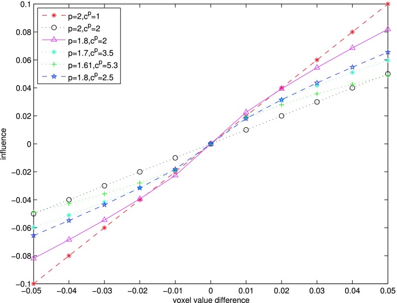
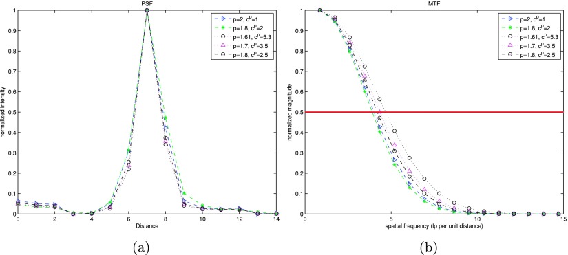
In Fig. 1, we compare the influence function of the quadratic regularization with those with several edge-preserving gGMRF priors. In the quadratic case (p = 2), the influence function is linear around the origin, which controls textures in a uniform manner. Reduced p retains better edge-preserving characteristics, since the influence function changes more slowly for larger voxel differences. The value c controls the inflexion point. Higher c pushes the edge-preserving behavior toward the origin. For example, to maintain similar influence to the quadratic with cp = 1 for differences of 0.01 which is considered the upper boundary of noise variation, the cp values for p = 1.8, p = 1.7, and p = 1.61 are set to 2.5, 3.5, and 5.3, respectively.
FIG. 1.
Influence function of the gGMRF regularization with different parameters.
2.B. Geometric configuration and forward and backprojection model
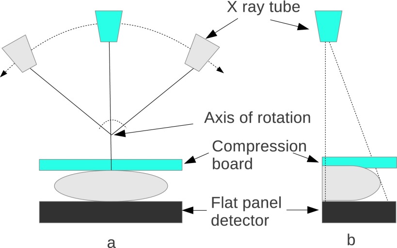
As shown in Fig. 2, a typical DBT system acquires 11 to 25 projections by rotating the x-ray tube around the center of rotation over an arc of less than 50° arc. In a motion synchronized with the position of the tube, the collimator is shifted during the acquisition, to confine the x-ray illumination area to the flat-panel detector. This detector, which remains stationary during the acquisition, is used to record images consisting of a large array of small pixels. Antiscatter grids are not usually used.
FIG. 2.
DBT imaging system: (a) front view; (b) side view.
The x-ray dose for a tomosynthesis exam is comparable to that for a one-view mammogram. In clinical tomosynthesis imaging, the breast of the patient is compressed in the same way as in mammography. The total image acquisition time is usually about 5 to 8 s.
The major advantage of statistical IRs is that they allow arbitrary specification of the system coefficient used in the statistical model described as Eq. (3). Any scanning geometry that uses only a short arc, including the cone-beam and flat-panel detector system above, can be accurately modeled by proper computation of the vector of system coefficients. The model can be designed to realistically represent the scanner, although this may come at great computational expense.
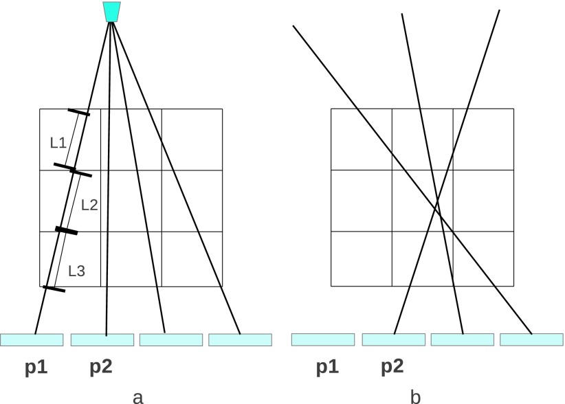
At the core of any efficient implementation of IR is the calculation of system coefficients in the forward and backward model, which often drives computation time and reconstruction accuracy. One of the models to calculate the system coefficient matrix is the distance driven approach,39 which accurately takes into account both the detector response and the voxel size. This method leads to fast implementation without degrading the frequency response and is considered to be a state-of-the-art approach. The distance driven technique may be applied in conjunction with a voxel-based iterative algorithm30 such as iterative coordination descent (ICD), where voxel calculations in each iteration require the related error sinograms to be updated by all other voxels. The inherent sequential processing makes the voxel-based algorithm hard to parallelize. Other algorithms such as in Ref. 40 or OS41 require a full independent forward and backprojection for each iteration, permitting easier parallelization. The ray-driven method, being the most favorable system model for this category of algorithms, is applied in this study. A typical 2D ray-driven forward model is illustrated in Fig. 3(a), where the image space is represented by a voxel mesh and the ray is modeled by a line connecting the source and the center of each detector element. The expected projection data are formalized as
| (10) |
where μj is the linear attenuation coefficient of the jth voxel along the ray path. An efficient ray-driven method was implemented based on the method proposed in the literature.42 A traversal algorithm along each ray is described by the ray equation: , where is the start point of the ray and denotes the ray direction vector. The ray is broken into intervals of t, each of which spans the whole voxel. To determine t, the ray length crossing the first vertical voxel boundary and the ray length intersecting the first horizontal voxel boundary are compared. The minimum of those two will indicate how much the ray travels within the current voxel. The intersected length within the current voxel is calculated by subtracting the last value of t from the current value of t. At the boundary, the adjacent voxel is identified and processing continues as before. A forward projection along a ray is defined as the inner product of intersection length vector and the linear attenuation coefficient for the corresponding voxel. The backprojection of a voxel is typically calculated by averaging the “on-path” projection data as shown in 3(b). Assuming that there are a total of M rays going through the jth voxel over all projection views, the backprojection of jth voxel bj is defined as
| (11) |
where pi denotes the projection data for the ith detector element; lij denotes the length of intersection of the ith ray model and jth voxel; and Li is the path length of the ray within the entire volume.
FIG. 3.
Ray-driven model: (a) ray-driven forward model; (b) ray-driven backprojection model.
2.C. Modified regularization design for predictable resolution property
The nonlinearity of the impulse response in statistical IR is often undesirable since it leads to an unpredictable and nonuniform resolution. In this section, we present an analytical form of the impulse response and demonstrate a way to linearize it to achieve predictable and uniform resolution. We start from a general quadratic regularization
| (12) |
The local impulse response of the reconstruction with a PL objective function shown as Eq. (4) and a quadratic penalty was previously derived43 as
| (13) |
where j denotes an impulse response at the jth voxel with the form of
μ(yi) is an estimator of μ on a noiseless measurement {yi}; A represents the system coefficient matrix; D(yi) is a diagonal matrix with the entry yi; HR is the Hessian matrix of R(μ); and ej is the jth unit vector. From Eq. (13), one can see that the impulse response Lj(μ) depends not only on the system coefficient and the penalty weight λ but also on the datasets associated with the incident x-ray and the object under scan. The data-sensitivity leads to a nonuniform impulse response, including shift-variant resolution and a data-dependent λ effect on the results. To reduce the data dependence, Fessler and Rogers proposed a modified penalty function43 for more uniform resolution. This penalty is written as
| (14) |
where ω is the weight assigned to ψ. κj is formalized for emission tomography as follows:
| (15) |
In x-ray transmission tomography, si, gij, qi are translated to si = 1, i ∈ [1, M], gij = lij, and qi = yi. To reduce the computational complexity, we propose a simplified version as follows:
| (16) |
where
| (17) |
since the condition of κk ≈ κj is obviously satisfied in the jth voxel’s neighbors. κ2 is roughly equivalent to a backprojection upon the data set {yi}.
We substituted Rm of Eq. (16) into Eq. (13). When an analogous deduction as in Fessler and Rogers43 is applied, Lj(μ) has the following form:
| (18) |
where I is an identity matrix. One can see that as the data weighting D(yi) is reduced to I, HRm, the Hessian matrix of Rm(μ), is transformed to HR, the Hessian matrix of R(μ). That means that the effect of λ on the impulse response from arbitrary measurements yi with the modified penalty is equivalent to the effect of λ on the impulse response with a uniform projection of yi = 1 with a quadratic penalty. In other words, pre-estimation using the measured data reduces the data-dependence terms and allows a predictable effect of λ on the reconstructed results.
Other work44 has shown that κ can also lead to improved uniformity in nonquadratic regularized reconstructions. Intuitively, κ reduces the data dependence in uniform regions. The edge-preserving effect on an impulse signal will vary as the difference changes between the signal and its background. As a result, the spatial resolution achieved by a quadratic regularization with specific λ values permits a baseline selection for nonquadratic regularized reconstruction allowing a degree of resolution uniformity while improving the resolution and noise trade-off over quadratic regularization.
2.D. Region-of-interest (ROI) reconstruction with super resolution
Statistical IR can recover fine details and small features more accurately than conventional algorithms. In order to fully utilize this advantage, a higher spatial resolution parameterization, specifically smaller voxels, needs to be applied to detect small features such as microcalcification. In this section, we develop high resolution reconstruction with the ray-driven method on an oversampling detector. As a result, intersected ray number and voxel number are significantly increased, such that extra computation is required. ROI reconstruction is an efficient option to concentrate computations only on the region that contains the interesting diagnostic details.
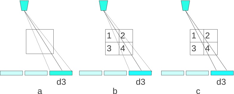
Practically, to increase the spatial resolution, voxels need to be divided into subvoxels. When the subvoxel dimension size becomes much smaller than the detector element size, the original ray-driven model, which represents a ray by a line connecting the source and the center of the corresponding detector element, is not accurate enough potentially causing resolution loss and a chess grid effect.45 Figure 4 demonstrates the undersampling situation and shows a potential solution as well. Figure 4(a) presents the forward model of a single voxel whose size is comparable to the detector element size. The dotted lines aligned at the two boundaries of the detector element represent the actual ray coverage. In this case, the intersection between the voxel and the line that connects the source and the center of the detector is accurate enough for forward and backprojection. In Fig. 4(b), one voxel is divided into four subvoxels in order to quadruple the resolution. According to the ray-driven model, the forward projection p is written as
| (19) |
where denotes the ray intersection with the corresponding subvoxel j whose attenuation coefficient is . Equation (19) shows that only subvoxels 1, 2, 4 are taken into account for the ray attenuation. In fact, all of these subvoxels should contribute to the ray attenuation according to the coverage of the dotted line. The ray-driven method with an oversampling detector46 may solve this problem. Instead of the ray being modeled as one line, it can be modeled as two lines, each of which connects the source and quarters of a detector element as shown in Fig. 4(c). The ray attenuation corresponding to the detector element d3 is calculated by the forward projection given by the two lines, which is
| (20) |
where , i ∈ 1, 2, denotes the intersection of each line within the jth subvoxel. Unlike Eq. (19), this calculation counts the effect from all subvoxels.
FIG. 4.
Ray-driven forward model for voxel and subvoxel: (a) ray-driven model for voxel; (b) ray-driven model for subvoxel; (c) oversampled ray-driven model for subvoxel.
The disadvantage of this oversampling detector based ray-driven method is that it significantly increases the computational cost, since more rays are required to be computed and more voxels are reconstructed. As a result, the high resolution reconstruction for the whole image volume is not very practical. Fortunately, the intensive computing is not necessary, since small features are only located in a small ROI. There has been much work on reconstruction within a small display field of view (DFOV) in CT.47,48 A typical approach involves a two-path reconstruction. The first path involves applying a pilot reconstruction with full field of view (FFOV) with a coarse voxel size. The second path involves updating the divided subvoxels in a smaller DFOV within that pilot reconstruction. The nonuniformity of voxel size usually leads to the partial volume problem resulting in data mismatch in the forward projection. The amount of the mismatch is determined by the implementation.
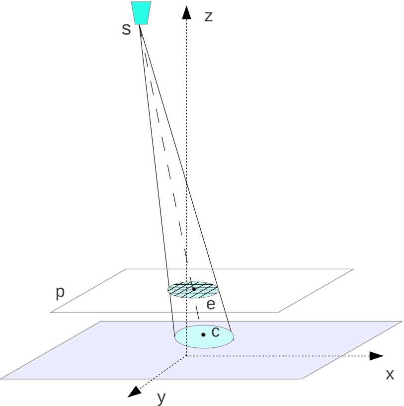
Compared to CT, in DBT, the image slice, which is parallel to the detector plane, is reconstructed transversely. Furthermore, the number of slices is relatively few ranging from 30 to 60 depending on slice thickness, and the angular range is typically less than 30°. These specific features allow an accurate ROI reconstruction without any pilot reconstruction. The key to this technique is (1) to generate a mask for each projection and use only the detector elements within the mask and (2) to estimate the minimum volume that needs to be updated for the ROI reconstruction. As demonstrated in Fig. 5, ROI in the plane p is marked by a circle with its center at e(xe, ye, ze) and a radius of re. A circular mask is projected on the projection data according to the tube position s(xs, ys, zs), which locates at the center c(xc, yc, zc). The value zc is 0 in the coordinate system. The center (xc, yc) may be mathematically written as
| (21) |
with radius
| (22) |
FIG. 5.
A circular mask, which is formed by projecting the ROI boundary along the ray beam, indicates the minimum data set required to reconstruct the voxels in ROI.
The circular mask in the projection domain indicates the minimum data set required to reconstruct the ROI. Therefore, the number of rays required for forward and backprojection is significantly reduced. In addition, only a small portion of volume, which covers all the ray paths in every circular mask, is necessary for iterative updates. Rough computing requirements given a typical DBT geometric configuration follow.
Suppose 15 projections of 2048 × 1664 each are taken and that the bin size is 0.14 mm. To reconstruct 60 slices of 1 mm thickness, a total of 200 megavoxels need to be updated in IR iterations, where each voxel is divided into a 0.14 × 0.14 × 1 mm grid. In contrast, consider a 7 × 7 mm ROI covering a lesion that requires high resolution review. A high spatial resolution ROI reconstruction with the voxel grid size of 0.07 × 0.07 × 1 mm can be performed. By applying our proposed method, only a 10 × 10 × 60 mm volume, which involves about 0.6 megavoxels, is necessary for an IR update. Based on our implementation, these computations take only seconds for all iterations. In addition, since the uniform and fine voxel size is applied along each ray path, there are less reconstruction artifacts associated with the partial volume effect. In this work, we adopt ROI reconstruction to reduce the computational complexity for high spatial resolution.
2.E. Computation of the solution
Through minimizing the objective function Eq. (4), one can estimate the optimal μ∗, which is formalized as follows:
| (23) |
With the choice of a strictly convex prior potential function, the cost function defined in Eq. (3) is strictly convex as well. ICD is an efficient algorithm to solve this problem. By representing the objective function as the second order Taylor series expansion,49 the objective function is approximated by a quadratic form which allows the high dimension optimization problem to be transferred to a sequential 1D optimal search. Interleaved nonhomogeneous and homogeneous voxel selection is used to speed up convergence by focusing the computation where it is most needed.30
The optimization-transfer (OT) based algorithm20 utilizes a series of separable surrogate parabolic functions lower bounded by the objective function. Minimization of Eq. (4) is transferred to minimization of these surrogate ones. We summarize the OT method as the following algorithm scheme:
| for each iteration t = 1, ..., Niter do | ||
| Find an surrogate function G(Θ, Φ) satisfying, | ||
| (1) G(Θt, Θt) = Ψ(Θt), | ||
| (2) Ψ(Θ) ≤ G(Θ, Θt), ∀Θt ≠ Θ, | ||
| we apply one step of Newton’s method on the surrogate, the optimal approximation at (t + 1)-th iteration is written as | ||
| ||
| end for |
where G(Θ, Θt) is a separable surrogate function lower bounded by Ψ(Θ) at Θt. The first Θ represents the linear attenuation coefficient vector μ. We use Θt+1 to represent the optimal Θ which leads to the smallest G(Θ, Θt). The “bounded” condition to form G(Θ, Θt) automatically leads to a monotonic convergence to the global optimal. ∇ΘG(Θt, Θt) represents the gradient toward the global optimal in the solution space. , which is the inverse of curvature of the separable surrogate function, denotes the search step size along each dimension. Due to the bounded condition, the curvature of the surrogate cannot be smaller than the curvature of the objective function, which results in a conservative step size.
The bounded condition is not necessary for monotonicity. In fact, a “nonbounded” surrogate with an aggressive step size is able to produce a monotonic convergence at faster rate. Some researchers have studied large step sizes. For example, an enlarged step size with the form of exponential power was proposed for ML-EM reconstruction.50 The algorithm lacks monotonicity, hence may have a problem with stability. The idea of over-relaxed step size was also mentioned in Yu et al.30 for the ICD framework, where a factor of 1 to 2 was used to scale up the step size. However, a larger step does not mean a faster convergence and might even lead to divergence.
A method for successively increasing over-relaxation in an OT based algorithm was proposed.51 Instead of a larger step size, an optimal step size, which produces the fastest convergence at each search step, was derived with the form of a scaled step size . An optimal scaling factor ρ∗ was defined as
| (25) |
where 0 ≤ σmin ≤ σmax ≤ 1 are the smallest and largest eigenvalues of the convergence matrix.51 The convergence rate is proportional to the largest eigenvalue.51 As iteration proceeds, the σmax has been demonstrated to change from 0 to 1, which means that the convergence speed is gradually slowing down as the estimate at each step is approaching the global optimal. Therefore, the optimal ρ∗ in Eq. (25) varied from 1 to K, a value larger than 1. That is, the optimal scaling factor ρ∗, which produces the optimal step size to achieve the fastest convergence rate at each iteration, is not scaled down gradually, but needs to be successively increased iteratively, which is fundamentally different from other methods50 where an exponential factor is supposed to be more conservative with increasing iterations.
The successively increasing over-relaxation OT based algorithm is proposed as follows:
| ρ = 1 and a = δ (δ > 1 can be adjusted in a specific case) |
| for each iteration t = 1, ..., Niter do |
| Calculate and |
| if then |
| ρ∗ = a and |
| else |
| ρ = 1 and |
| end if |
| end for |
ΘNEW is updated by a ρ-scaled difference between ΘT and the last iteration’s estimate. In image reconstructions, ΘT represents the linear attenuation vector μ, which can be updated by using the separable surrogate technique.20 Using this technique, we derived the iterative estimate of μ with the gGMRF prior in the following form:
| (26) |
where κ is precalculated (before iteration starts) by the backprojection operation as shown in Eq. (17); λ represents the penalty weight in the place of Eq. (4); and p and c values are important parameters to control the trade-offs between the edge-preserving behavior and noise reduction. By comparing the objective functions Ψ(ΘT) and Ψ(ΘNEW), the update strategy and ρ are determined. If Ψ(ΘNEW) is less than Ψ(ΘT), meaning the scaled solution is closer to the optimal in the solution space, then Θ is updated by ΘNEW and ρ is increased by a multiplier a. Otherwise, ΘT is used to update Θ, and ρ is set to 1. For each iteration step, the algorithm always uses the choice that achieves a faster convergence. For instance, an acceleration with a factor ϵ is gained in one iteration. After M iterations, an exponential gain of ϵM is achieved.
Given that a representative OT based method requires full forward and backprojection for each iteration, our proposed method requires one extra voxel update. This update is performed concurrently with the original one, with a low computational cost. In addition, the calculations of Ψ(ΘNEW) and Ψ(ΘT) can reuse the error sinogram and the update operations. The efficiency of the proposed algorithm framework has been demonstrated in our previous work.51
3. METHODS AND MATERIALS
3.A. System description
We acquired data on the stationary DBT prototype system7,8 to assess the performance of the proposed method. In this system, a flat-panel detector is used for image acquisition. The origin of the 3D coordinate system is located at the center of the detector. With a 140 μm detector element pitch, the total projection size is 2048 × 1661. Multiple x-ray beams are positioned along a straight line parallel to the detector plane. The detector is 690 mm from the source, which is designed to have 15 x-ray beams spanning a distance of 323.8 mm from end to end. The linear spacing between the x-ray beams varies to provide a regular 2° angular step size.
Breast phantoms were scanned on a stage with a 25.4 mm air gap. Projections were acquired using 28 kVp, a molybdenum filter, a molybdenum target, and 20 mAs per projection.
3.B. Reconstructions for comparison study
In the comparison study, we compared FBP, SART, and OS MLEM (OS-EM) with the proposed statistical IR. In the remainder of this paper, we use the acronym SIR-ρ-OT to refer to the proposed statistical IR, i.e., the successively increasing over-relaxation ρ-based OT (ρ-OT) algorithm for solving the estimation problem posed by SIR.
FBP based reconstruction is widely used in current commercial DBT products. Since FBP has a linear response, tuning the filter kernel permits a desired trade-off between resolution and noise. As a standard reference method, we applied a sampling density based ramp filter52 and a Hanning filter to remove the ring effects and high frequency noise. The kernel was applied on each row of projection data in the path direction of the x-ray tube, and then the 3D volume was reconstructed by a pixel-driven backprojection.
Unlike the FBP algorithm, which is a one-step operation, iterative algorithms such as SART and OS-EM perform the reconstruction in a recursive fashion. During the iterations, a 3D ray-driven method was employed for forward and backprojection. The number of iterations was determined based on a semiquantitative method.53 According to the method, curves of objective function versus iterations, noise versus contrast as iteration proceeds and artifact spread function (ASF)6 were drawn in a phantom study with the scanner. The number of iterations was chosen based on those performance curves.
As a reference algorithm, SART is initiated by a backprojection and uses eight iterations, each of which is completed by going through all projections sequentially. For an OS based method, there is usually fast convergence at the early iterations but eventually oscillation around the global optimal solution. To gain the initial acceleration and avoid the oscillation, we utilized three iterations with ordered subsets, followed by eight iterations with full data sets.
Our proposed statistical IR is solved by the successively increasing over-relaxation OT framework described in Sec. 2 with the iterative solution of Eq. (26). According to experiments in the literature,35 λ = 8 provided the best trade-off in maintaining resolution and reducing noise among all investigated λ for the quadratic regularization. Using the edge-preserving penalty with this same λ, the performance can be further enhanced to achieve a better resolution with the same amount of noise reduction. Three iterations with ordered subsets, each of which consists of an individual projection, are used to start the estimation process and subsequently five iterations with full data sets are performed with the ρ-OT framework. One trick is utilized in our implementation, where instead of scaling up step size for all voxels in the same manner, we only enlarge the step size of those presenting high frequency features. Therefore, the voxel update in the most variable regions, such as edges between high and low-contrast and details within a complex background, contributes more to the decrease of objective function value, which leads to a faster convergence in these regions. The details of the update strategy will be given in another paper.
3.C. Parameter optimization of IR model
The form of the gGMRF prior introduced in Sec. 2 depends on two parameters: p, which controls the degree of curvature in the influence function in low- and high-contrast regions, and c, which determines the threshold between the two types of regions. To seek the optimal parameter combination, reconstructions of a homogeneous breast phantom were performed with multiple parameter choices. They were p = 2, cp = 1; p = 1.8, cp = 2; p = 1.8, cp = 2.5; p = 1.7, cp = 3.5; and p = 1.61, cp = 5.3. Point spread function (PSF) and contrast to noise ratio (CNR) were applied to measure the results of these parameter combinations. The case in which p = 2, cp = 1 specifies a quadratic regularization. The reconstruction from the quadratic parameter combination was chosen as the baseline.
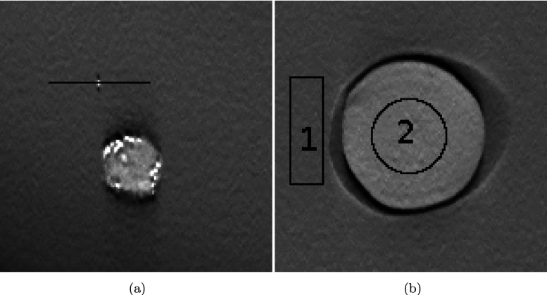
The PSF curves presented in Fig. 6(a) were measured by forming profiles through the isolated microcalcification shown in Fig. 7(a). These curves were then fitted into the Gaussian functions to remove noise. The Fourier transform of the fitted function is the modulation transfer function (MTF), as shown in Fig. 6(b). The spatial frequency at 50% MTF peak is used to describe the in-plane spatial resolution. As discussed in Sec. 2, a smaller p tends to introduce more edge-preserving behavior toward the high contrast region. By increasing c, the inflexion is pulled closer to the origin to improve the low-contrast detectability. Among all parameter combinations for SIR-ρ-OT, the parameter set p = 1.61, c = 5.3 presents the best frequency response which is 18% higher than the baseline. To investigate the contrast sensitivity, CNR is calculated by subtracting the mean value in the background marked as region 1 [Fig. 7(b)] from the mean value in the mass region marked as 2, and then dividing the standard deviation of the background.
FIG. 6.
Spatial resolution measured along microcalcification on a focus plane reconstructed by SIR-ρ-OT with selected parameter combinations. (a) PSF curves; (b) MTF curves.
FIG. 7.
Measurement of PSF and CNR: (a) microcalcification, used to measure PSF; (b) a mass object and its background, used to calculate CNR.
The CNR and half-width of 50% MTF above are summarized in Table I, which shows that, in terms of CNR, all edge-preserving parameter combinations performed better than the baseline reconstruction. The case of p = 1.61, cp = 5.3 produced the second highest CNR and led to the highest resolution. The parameter combination p = 1.8, cp = 2 produced the highest CNR but yielded a slightly worse spatial resolution than the baseline. Based on these observations, p = 1.61, cp = 5.3 may be a good compromise between contrast sensitivity and resolution. This is the parameter set that was adopted in the rest of experiments.
TABLE I.
CNR and in-plane MTF for SIR-ρ-OT with selected parameter combinations.
| Parameters | CNR | HWHM of MTF |
|---|---|---|
| p = 2, c = 1 (quadratic) | 6.1601 | 4.0063 |
| p = 1.8, cp = 2 | 12.4267 | 3.9041 |
| p = 1.8, cp = 2.5 | 6.5769 | 4.1951 |
| p = 1.7, cp = 3.5 | 7.3294 | 4.3324 |
| p = 1.61, cp = 5.3 | 7.5906 | 4.6825 |
4. EXPERIMENTS AND RESULTS
4.A. Improvement in detectability
In this section, experiments comparing detectability are conducted with a breast phantom composed of a tissue equivalent, complex, heterogeneous background, containing an assortment of microcalcifications, fibrils, and masses, where the grain size of microcalcifications varies from 0.130 to 0.275 mm. All reconstructed results are presented in comparable display windows. For IR methods, the display window was set to [0.0490, 0.0601]. For FBP, it was set to [1.3660, 1.3714]. The reason for the shifting is that, without performing data matching, the reconstruction error from FBP was deteriorated due to the highly incomplete sampling.
Results reconstructed by SIR-ρ-OT with the optimized parameters were compared against those generated from the reference methods. A nonprewhitening (matched filter) observer signal-to-noise ratio (SNR)54 model is adopted to evaluate the microcalcification visibility. To fully demonstrate the advantage of SIR-ρ-OT, ROI reconstruction with higher resolution was deployed as well, where the transverse voxel size in the ROI was reduced to 0.07 mm, which is half of the detector element size. The reconstructed results were then compared to those with the original voxel size.
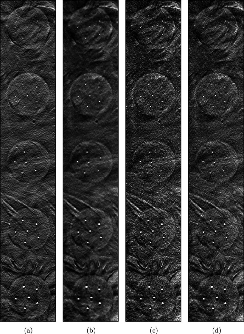
Figure 8 presents the comparison of microcalcifications in circular masses reconstructed by the different methods. Each row represents reconstructions of microcalcifications of a different size, from 0.165 mm (top) to 0.275 mm (bottom). In the first row, the six microcalcifications can be seen clearly when the mass is reconstructed by SIR-ρ-OT in (b) but not when it is reconstructed by FBP in (a). This difficulty in detection is caused by insufficient spatial resolution. Although OS-EM in (c) and SART in (d) produce resolution as high as the proposed method, the microcalcifications reconstructed by each of these methods are somewhat hidden in the noisy background. Similar situations can be observed in the second and third rows. The microcalcifications in the fourth and fifth rows are large enough to be detected among all methods.
FIG. 8.
Comparison of microcalcification in mass reconstructed by different methods. (a) FBP, (b) SIR-ρ-OT, (c) OS-EM, (d) SART.
To validate the microcalcification detectability improvement of our proposed method, we employed the nonprewhitening (matched filter) observer SNR for a signal-known-exactly/background-known-exactly (SKE/BKE) task. This model is given as
| (27) |
where denotes the conditional mean of a statistic λ given that microcalcification is present or absent. Regarding this task, we use f+ to represent a vectorized image patch that includes a single microcalcification. λ+ is then calculated as the inner product of f+ and a signal-present template w, which is created by binarizing the mean value of all signal-present f+. In the same manner, λ− is computed as the inner product of f− which is a microcalcification free image vector and w. The is then computed by averaging each of the signal responses with the same template applied. In addition, , where K+ is the covariance of all applied f+.
We scanned the phantom three times with the same acquisition parameters. Volumes were reconstructed by each approach. To calculate the SNR for microcalcification of each size, a 6 by 6 image patch containing the microcalcification was vectorized. There are six microcalcifications for each size available in one mass as shown in Fig. 8. Hence, a total of 18 image patches can be used to calculate the . was computed by using 180 image patches over multiple reconstruction slices. Covariance was computed from 800 images collected from different locations and multiple adjacent reconstruction slices. In order to obtain a larger number of ROIs, we assumed that σ+ and σ− are identical. Such assumptions are valid in the limit of small signals but may be violated for larger signals. Due to a small number of data sets available to compute σ+, however, we invoked the assumptions for all microcalcification sizes to avoid bias in covariance estimation.
A comparison of the SNR results of all methods is summarized in Table II. The values in the table align with our observations. For example, in agreement with our observation that small microcalcifications in the second rows could be more easily detected using the SIR-ρ-OT method, the observer SNR value corresponding to SIR-ρ-OT is obviously higher than that of its competitors: 34% higher than the SNR value for FBP and over 20% higher than that for other IR methods. The SNR values in rows 3, 4, and 5, which represent easier detection tasks, are only slightly different among all methods.
TABLE II.
Nonprewhitening (matched filter) observer SNR measured on microcalcifications within mass as shown in Fig. 8.
| FBP | SIR-ρ-OT | OS-EM | SART | |
|---|---|---|---|---|
| Row 1 | 12.2 | 15.5 | 13.7 | 14.3 |
| Row 2 | 24.4 | 32.8 | 25.2 | 26.9 |
| Row 3 | 33.0 | 35.4 | 32.9 | 34.4 |
| Row 4 | 36.3 | 38.0 | 36.4 | 36.1 |
| Row 5 | 47.5 | 48.7 | 44.9 | 46.2 |
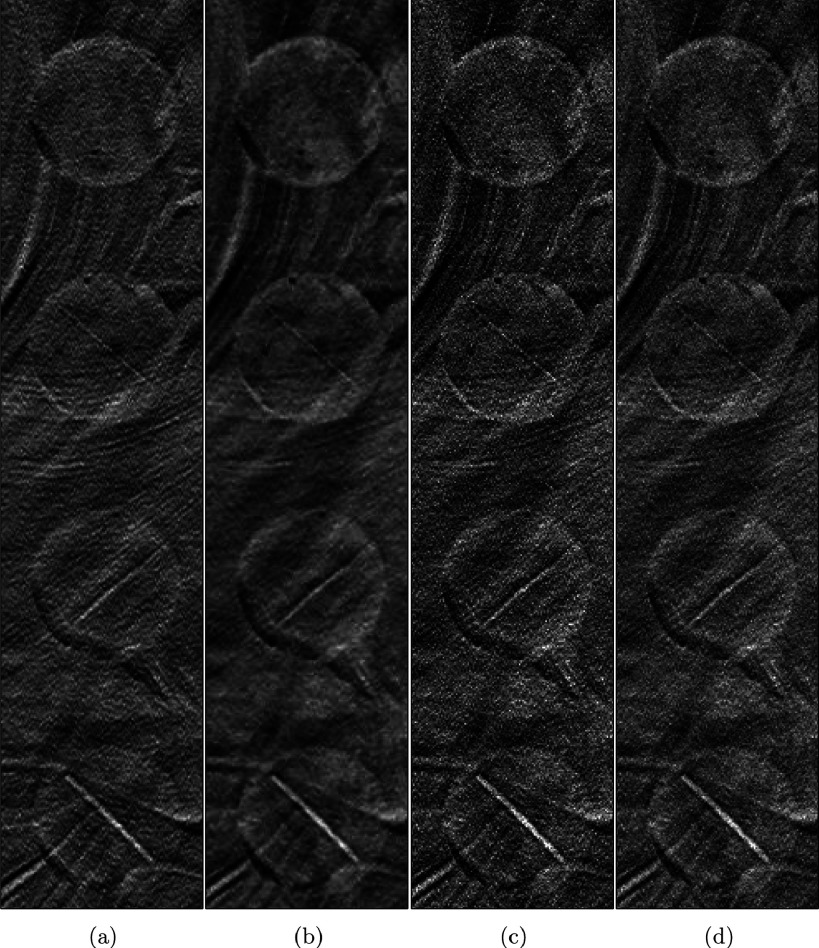
Figure 9 presents the comparison of fibrils in circular masses reconstructed by each method. All fibrils in these results are detectable. Compared with the results of FBP reconstruction in (a), SIR-ρ-OT produces a much clearer boundary and enhanced contrast for each mass. The results of OS-EM in (c) and SART reconstruction in (d) present relatively high noise which makes the boundaries of fibrils more obscure.
FIG. 9.
Comparison of fibrils in mass reconstructed by different methods. (a) FBP, (b) SIR-ρ-OT, (c) OS-EM, (d) SART.
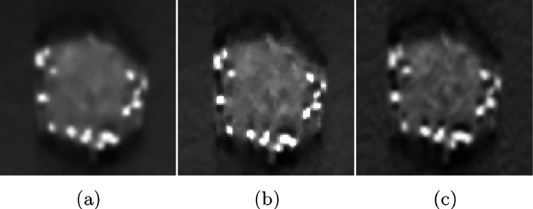
Figure 10 shows an 8.4 × 8.4 mm area that includes multiple microcalcifications embedded in a mass. Compared to FBP reconstruction with low spatial resolution shown in Fig. 10(c), SIR-ρ-OT reconstruction with low spatial resolution, shown in Fig. 10(a), significantly reduces the noise in the soft tissue. The image reconstructed by SIR-ρ-OT with high resolution is shown in Fig. 10(b). Comparing (b) to (a) and (c), we notice that the slowly varying area in the image presents a little higher noise than (a) but still lower than (c). The most significant difference is the reconstruction of the microcalcifications. (b) shows the sharpest edge for each microcalcification among all competitors.
FIG. 10.
Zoomed focus plane with a mass and several granular microcalcification. (a) SIR-ρ-OT with low resolution, (b) SIR-ρ-OT with high resolution, (c) FBP with low resolution.
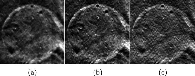
The high spatial resolution reconstruction was also applied in a ROI with small, barely visible objects. Figure 11 presents reconstructed images where six smaller microcalcifications of 0.130 mm are located in a circular mass within a 14 × 14 mm area. The small objects are highly obscured in the results of low-resolution IR shown in (a) and low-resolution FBP shown in (c). The nonvisibility is mainly caused by insufficient spatial resolution. As shown in (b), SIR-ρ-OT with high resolution led to better detectability than did the other two methods. In fact, it led to all of the small objects being visible. The higher noise in 11(b) could be better suppressed by applying a larger λ.
FIG. 11.
Zoomed focus plane with a circular mass and six tiny microcalcification. (a) SIR-ρ-OT with low resolution, (b) SIR-ρ-OT with high resolution, (c) FBP with low resolution.
4.B. Performance for in-plane resolution/noise trade-offs
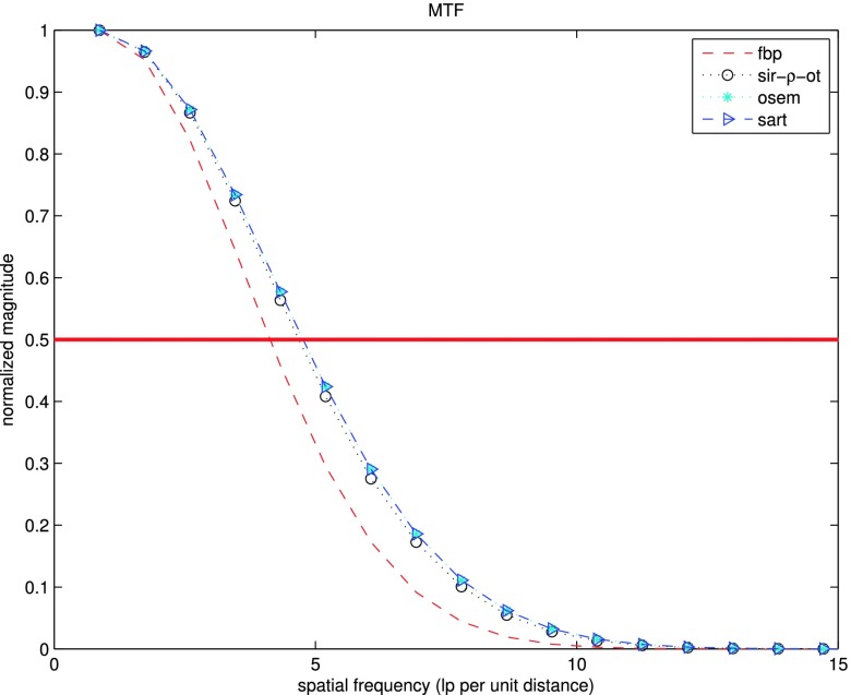
For a comparison of in-plane properties at equal resolution between the reference methods and the proposed method, we reconstructed the image shown in Fig. 7(a). In-plane MTF was calculated. The standard deviation of noise was measured in a homogeneous region shown in Fig. 7(b). The CNR was evaluated for the regions in Fig. 7(b). Results are presented in Fig. 12 and Table III.
FIG. 12.
In-plane MTF measured along microcalcification on a focus plane reconstructed by SIR-ρ-OT, FBP, SART, and OS-EM.
TABLE III.
Comparison of in-plane MTF, noise, and CNR for SIR-ρ-OT and the reference methods.
| FBP | SIR-ρ-OT | SART | OSEM | |
|---|---|---|---|---|
| 50% MTF | 4.134 | 4.683 | 4.766 | 4.766 |
| 10% MTF | 6.836 | 7.807 | 7.988 | 7.988 |
| Standard deviation (10−4) | 7.747 | 6.644 | 18.713 | 17.532 |
| CNR | 2.663 | 7.590 | 4.550 | 4.498 |
The measured in-plane MTF for SIR-ρ-OT was comparable to that of the SART and OS-EM images, and better than that of the FBP image. SIR-ρ-OT presented a 60%–70% noise reduction compared with SART and OS-EM. Furthermore, SIR-ρ-OT provided the best CNR performance among all methods: close to 1.7 times as high as the performance of SART and OS-EM, and 3 times as high as FBP.
4.C. Reduction of cross-plane artifacts
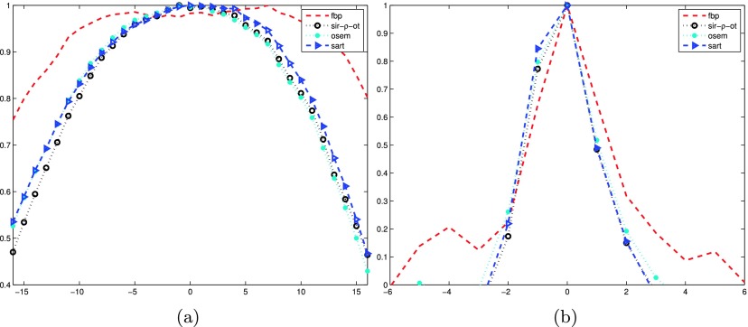
We calculated ASF6 to evaluate image blur in the Z direction that is perpendicular to the X–Y detector plane. The image blur is mainly introduced by the highly undersampled geometry. ASF is defined as the ratio of the CNR values between the off-plane layer and the in-plane layer. The measurement was performed on a breast phantom with a homogeneous background.
Figure 13 shows the ASF curves of the selected mass and the microcalcification shown in Fig. 7. The layers at negative distances denote the image slices below the feature layer, and those at positive distances denote image slices above. The FBP results produced a slowly decreasing ASF curve, indicating a strong interplane blurring effect for the mass object. SIR-ρ-OT, OS-EM, and SART results, on the other hand, produced ASF curves that dropped quickly as the distance from the feature increased, indicating that these techniques are superior in suppressing interplane blurring.
FIG. 13.
Comparison of ASF curves of the selected mass and microcalcification in the results reconstructed by FBP, SIR-ρ-OT, OS-EM, and SART. (a) ASF curve of mass object; (b) ASF curve of microcalcification object.
With the microcalcification, all four methods had comparable ASF behaviors at the off-plane close to the in-plane layer. However, at the off-planes farther away from the in-plane layer, the curve from the FBP reconstruction tends to decrease slowly, whereas those from the other three methods decreased more quickly, indicating that those methods were better at mitigating the cross-plane artifacts. SIR-ρ-OT showed slightly fewer cross-plane artifacts than the other IRs.
The difference between the FBP reconstruction curve and the other curves was greater in the mass ASF plot versus the microcalcification plot. This behavior was predictable. In Fourier space, the frequency contents of a large object may be more varied in magnitude than those of a small object. As a result, the small object could be restored much more easily than the larger object, when the same Fourier space sampling was used.
5. DISCUSSION AND CONCLUSION
We have presented multiple key statistical IR techniques for DBT image reconstruction. The effects of the penalty weight λ on the appearance of the reconstructed images were fully investigated using a quadratic regularization with a precomputed parameter κ. κ was also extended to incorporate our proposed gGMRF prior. This prior provides flexibility in its parameters necessary to control the behavior both around the origin and at the tails of the distribution. Our experiments show that a superior trade-off between resolution and noise could be achieved by optimizing the parameter combination of p and c. Based on an efficient ray-driven model, we proposed an oversampling technique on the detector elements that can improve the reconstruction accuracy for high spatial resolution and hence enable improved detectability of microcalcifications whose grain size is smaller than the detector element size.
According to our phantom studies, in which we used a nonprewhitening (matched filter) observer metric and visual comparisons, our proposed statistical IR performed better than traditional approaches in difficult detection tasks. Compared to other IR methods such as SART and OS-EM, the proposed SIR-ρ-OT method provided comparable spatial resolution with improved CNR performance. These benefits, together with those described above, potentially improve the ability to detect small microcalcifications and reveal low-contrast lesions in clinical applications. In addition, compared to FBP, all IR methods can effectively reduce interplane blurring and artifacts with better ASF behavior, and significantly improve object conspicuity by removing the overlapping structures.
A practical ROI reconstruction with high spatial resolution was applied to reduce the number of rays and the number of reconstructed voxels. Based on our preliminary evaluation, this solution profoundly lowers the computational complexity and the memory used. However, since IR-based methods still need multiple iterations to be convergent, convergence rate remains a challenge for clinical applications. An efficient OT-based algorithm framework with a successively increasing over-relaxation was discussed together with the convergence analysis. This method potentially allows fewer iterations to achieve decent image quality and acceptable convergence.
Recent progress in hardware and parallel computing allows the realization of the computationally expensive statistical IR in clinical applications. Hardware accelerations will enable the superior image quality provided by the proposed statistical IR. Future works will be conducted to investigate these hardware accelerations in order to benefit diagnostics in real clinical applications.
ACKNOWLEDGMENTS
This work is partly supported by Grant No. NIH/NCI R01 CA134598-01A1. Shiyu Xu wants to thank Dr. Santosh Kulkarni and Debashish Pal, both at GE Healthcare, and Dr. J. Webster Stayman, in Biomedical Engineering at Johns Hopkins University, for their valuable comments.
REFERENCES
- 1.BreastCancer.org, “U.S. Breast Cancer Statistics,” available at http://www.breastcancer.org (2015), accessed July-18-2015.
- 2.Holland R., Mravunac M., Hendriks J. H., and Bekker B. V., “So-called interval cancers of the breast: Pathologic and radiologic analysis of sixty-four cases,” Cancer 49, 2527–2533 (1982). [DOI] [PubMed] [Google Scholar]
- 3.Dobbins J. T. and Godfrey D. J., “Digital X-ray tomosynthesis: Current state of the art and clinical potential,” Phys. Med. Biol. 48(19), 65–106 (2003). 10.1088/0031-9155/48/19/R01 [DOI] [PubMed] [Google Scholar]
- 4.Dobbins J. T., “Tomosynthesis imaging: At a translational crossroads,” Med. Phys. 36(6), 1956–1967 (2009). 10.1118/1.3120285 [DOI] [PMC free article] [PubMed] [Google Scholar]
- 5.Chen Y., “Digital breast tomosynthesis (DBT)—A novel imaging technology to improve early breast cancer detection: Implementation, comparison and optimization,” Ph.D. thesis,Department of Electrical Computer Engineering, Duke University, 2007. [Google Scholar]
- 6.Zhang Y., “A comparative study of limited-angle cone-beam reconstruction methods for breast tomosynthesis,” Med. Phys. 33, 3781–3795 (2006). 10.1118/1.2237543 [DOI] [PMC free article] [PubMed] [Google Scholar]
- 7.Qian X., Rajaram R., Calderon-Colon X., Yang G., Phan T., Lu D. S. L. J., and Zhou O., “Design and characterization of a spatially distributed multibeam field emission x-ray source for stationary digital breast tomosynthesis,” Med. Phys. 36, 4389–4399 (2009). 10.1118/1.3213520 [DOI] [PMC free article] [PubMed] [Google Scholar]
- 8.Tucker A. W., Lu J., and Zhou O., “Dependency of image quality on system configuration parameters in a stationary digital breast tomosynthesis system,” Med. Phys. 40(3), 031917 (10pp.) (2013). 10.1118/1.4792296 [DOI] [PMC free article] [PubMed] [Google Scholar]
- 9.Xu S., Cong L., Chen Y., Lu J., and Zhou O., “Breast tomosynthesis imaging configuration optimization based on computer simulation,” J. Electron. Imaging 23(1), 013017 (2014). 10.1117/1.JEI.23.1.013017 [DOI] [Google Scholar]
- 10.Turbell H., “Cone-beam reconstruction using filtered backprojection,” Ph.D. thesis,Department of Electrical Engineering, Linkoping University, 2001. [Google Scholar]
- 11.Candes E. J., Romberg J., and Tao T., “Robust uncertainty principles: Exact signal reconstruction from highly incomplete frequency information,” IEEE Trans. Inf. Theory 52, 489–509 (2006). 10.1109/TIT.2005.862083 [DOI] [Google Scholar]
- 12.Zeng G. L., “A filtered backprojection algorithm with characteristics of the iterative landweber algorithm,” Med. Phys. 39(2), 603–607 (2012). 10.1118/1.3673956 [DOI] [PMC free article] [PubMed] [Google Scholar]
- 13.Mertelmeier T., Orman J., Haerer W., and Dudam M. K., “Optimizing filtered backprojection reconstruction for a breast tomosynthesis prototype device,” Proc. SPIE 6142, 61420F (2006). 10.1117/12.651380 [DOI] [Google Scholar]
- 14.Andersen A. H. and Kak A. C., “Simultaneous algebraic reconstruction technique (SART): A superior implementation of the art algorithm,” Ultrason. Imaging 6, 81–93 (1984). 10.1177/016173468400600107 [DOI] [PubMed] [Google Scholar]
- 15.Andersen A. H., “Algebraic reconstruction in CT from limited views,” IEEE Trans. Image Process. 8, 50–55 (1989). 10.1109/42.20361 [DOI] [PubMed] [Google Scholar]
- 16.Bertero M., Poggio T. A., and Torre V., “Ill-posed problems in early vision,” Proc. IEEE 76(8), 869–889 (1988). 10.1109/5.5962 [DOI] [Google Scholar]
- 17.Lange K., Bahn M., and Little R., “A theoretical study of some maximum likelihood algorithms for emission and transmission tomography,” IEEE Trans. Med. Imaging 6, 106–114 (1987). 10.1109/TMI.1987.4307810 [DOI] [PubMed] [Google Scholar]
- 18.Lange K. and Fessler J. A., “Globally convergent algorithms for maximum a posteriori transmission tomography,” IEEE Trans. Med. Imaging 4(10), 1430–1438 (1995). 10.1109/83.465107 [DOI] [PubMed] [Google Scholar]
- 19.Pierro A. D., “On the relation between the ISRA and the EM algorithm for positron emission tomography,” IEEE Trans. Med. Imaging 12, 328–333 (1993). 10.1109/42.232263 [DOI] [PubMed] [Google Scholar]
- 20.Erdogan H. and Fessler J. A., “Monotonic algorithms for transmission tomography,” IEEE Trans. Med. Imaging 18, 801–814 (1999). 10.1109/42.802758 [DOI] [PubMed] [Google Scholar]
- 21.Fessler J. A., “Iterative method for image reconstruction,” EECS Department, The University of Michigan, ISBI Tutorial, April 6, 2006.
- 22.Elbakri I. A. and Fessler J. A., “Efficient and accurate likelihood for iterative image reconstruction in X-ray computed tomography,” Proc. SPIE 5032(3), 480–492 (2003). 10.1117/12.480302 [DOI] [Google Scholar]
- 23.Elbakri I. A. and Fessler J. A., “Statistical X-ray computed tomography image reconstruction with beam hardening correction,” Proc. SPIE 4322, 1–12 (2001). 10.1117/12.430961 [DOI] [Google Scholar]
- 24.Fessler J. A., “Grouped coordinate descent algorithms for robust edge-preserving image restoration,” Proc. SPIE 3170, 184–194 (1997). 10.1117/12.279713 [DOI] [Google Scholar]
- 25.Fessler J. A., “Penalized weighted least-squares image reconstruction for positron emission tomography,” IEEE Trans. Med. Imaging 13, 290–300 (1994). 10.1109/42.293921 [DOI] [PubMed] [Google Scholar]
- 26.Thibault J.-B., Sauer K. D., Bouman C. A., and Hsien J., “A three-dimensional statistical approach to improved image quality for multislice helical CT,” Med. Phys. 34(11), 4526–4544 (2007). 10.1118/1.2789499 [DOI] [PubMed] [Google Scholar]
- 27.LaRoque S. J., Sidky E. Y., and Pan X., “Accurate image reconstruction from few-views and limited-angle data in divergent-beam CT,” JOSA A 25(7), 1772–1782 (2008). 10.1364/JOSAA.25.001772 [DOI] [PMC free article] [PubMed] [Google Scholar]
- 28.Tian Z., Jia X., Yuan K., Pan T., and Jiang S. B., “Low-dose CT reconstruction via edge-preserving total variation regularization,” Phys. Med. Biol. 56(18), 5949–5967 (2011). 10.1088/0031-9155/56/18/011 [DOI] [PMC free article] [PubMed] [Google Scholar]
- 29.Stayman J. W., Otake Y., Prince J. L., Khanna A. J., and Siewerdsen J. H., “Model-based tomographic reconstruction of objects containing known components,” IEEE Trans. Med. Imaging 31, 1837–1848 (2012). 10.1109/TMI.2012.2199763 [DOI] [PMC free article] [PubMed] [Google Scholar]
- 30.Yu Z., Thibault J.-B., Bouman C. A., Sauer K. D., and Hsien J., “Fast model-based x-ray CT reconstruction using spatially non-homogeneous ICD optimization,” IEEE Trans. Image Process. 20(1), 161–175 (2011). 10.1109/TIP.2010.2058811 [DOI] [PubMed] [Google Scholar]
- 31.Wu T., “Tomographic mammography using a limited number of low-dose cone-beam projection images,” Med. Phys. 30, 365–380 (2003). 10.1118/1.1543934 [DOI] [PubMed] [Google Scholar]
- 32.Das M., Gifford H. C., O’Connor J. M., and Glick S. J., “Penalized maximum likelihood reconstruction for improved microcalcification detection in breast tomosynthesis,” IEEE Trans. Med. Imaging 30, 904–914 (2011). 10.1109/TMI.2010.2089694 [DOI] [PMC free article] [PubMed] [Google Scholar]
- 33.Xu S. and Chen Y., “Compton scattering suppression based image reconstruction method for digital breast tomosynthesis,” in IEEE International Workshop on Genomic Signal Processing and Statistics (IEEE, 2011), pp. 190–193. [Google Scholar]
- 34.Xu S. and Chen Y., “An simulation based image reconstruction strategy with predictable image quality in limited-angle X-ray,” Proc. SPIE 8668, 86685P (2013). 10.1117/12.2007976 [DOI] [Google Scholar]
- 35.Xu S., Chen Y., Lu J., and Zhou O., “An application of pre-computed backprojection based penalized-likelihood image reconstruction on stationary digital breast tomosynthesis,” Proc. SPIE 8668, 86680V (2013). 10.1117/12.2007981 [DOI] [Google Scholar]
- 36.Hsieh J., Computed Tomography: Principles, Design, Artifacts, and Recent Advances (SPIE, Bellingham, WA, 2009). [Google Scholar]
- 37.Bouman C. A. and Sauer K., “A generalized Gaussian image model for edge-preserving MAP estimation,” IEEE Trans. Image Process. 2, 296–310 (1993). 10.1109/83.236536 [DOI] [PubMed] [Google Scholar]
- 38.Xu S., Inscoe C. R., Lu J., Zhou O., and Chen Y., “Pre-computed backprojection based penalized-likelihood (PPL) reconstruction with an edge-preserved regularizer with stationary digital breast tomosynthesis,” Proc. SPIE 9033, 903359 (2014). 10.1117/12.2043772 [DOI] [Google Scholar]
- 39.Man B. D. and Basu S., “Distance-driven projection and backprojection in three dimensions,” Phys. Med. Biol. 49(11), 2463–2475 (2004). 10.1088/0031-9155/49/11/024 [DOI] [PubMed] [Google Scholar]
- 40.Mumcuoglu E. U., Leahy R., Cherry S. R., and Zhou Z., “Fast gradient-based methods for Bayesian reconstruction of transmission and emission PET images,” IEEE Trans. Med. Imaging 13(4), 687–701 (1994). 10.1109/42.363099 [DOI] [PubMed] [Google Scholar]
- 41.Erdogan H. and Fessler J. A., “Ordered subsets algorithms for transmission tomography,” Phys. Med. Biol. 44, 2835–2851 (1999). 10.1088/0031-9155/44/11/311 [DOI] [PubMed] [Google Scholar]
- 42.Amanatides J. and Woo A., “A fast voxel traversal algorithm for ray tracing,” Proc. Eurographics 87, 3–10 (1987). [Google Scholar]
- 43.Fessler J. A. and Rogers W. L., “Resolution properties of regularized image reconstruction methods,” Technical Report 297, Communication and Signal Processing Laboratory, Department of EECS, University of Michigan, Ann Arbor, MI 48109-2122, 1995.
- 44.Ahn S. and Leahy R. M., “Spatial resolution properties of nonquadratically regularized image reconstruction for PET,” in 3rd IEEE International Symposium on Biomedical Imaging: Macro to Nano (IEEE, 2006), pp. 287–290. [Google Scholar]
- 45.Miao C., “Comparative studies of different system models for iterative CT image reconstruction,” Ph.D. thesis, Wake Forest University, 2013. [Google Scholar]
- 46.Zhuang W., Gopal S., and Hebert T. J., “Numerical evaluation of methods for computing tomographic projections,” IEEE Trans. Nucl. Sci. 41(4), 1660–1665 (1994). 10.1109/23.322963 [DOI] [Google Scholar]
- 47.Hamelin B., Goussard Y., Cloutier J.-P. D. G., Beaudoin G., and Soulez G., “Design of iterative ROI transmission tomography reconstruction procedures and image quality analysis,” Med. Phys. 37(9), 4577–4589 (2010). 10.1118/1.3447722 [DOI] [PubMed] [Google Scholar]
- 48.Yu Z., Thibault J.-B., Bouman C. A., Sauer K., and Hsieh J., “Edge localized iterative reconstruction for computed tomography,” in Proceedings of the 10th International Meeting on Fully Three-Dimensional Image Reconstruction in Radiology and Nuclear Medicine (IEEE, 2009). [Google Scholar]
- 49.Yu Z., Thibault J.-B., Bouman C. A., Sauer K. D., and Hsien J., “Accelerated line search for coordinate descent optimization,” IEEE Nucl. Sci. Symp. Conf. Rec. 5, 2841–2844 (2006). 10.1109/NSSMIC.2006.356469 [DOI] [Google Scholar]
- 50.Hwang D. and Zeng G. L., “Convergence study of an accelerated ML-EM algorithm using bigger step size,” Phys. Med. Biol. 51, 237–252 (2006). 10.1088/0031-9155/51/2/004 [DOI] [PubMed] [Google Scholar]
- 51.Xu S., Zhang Z., and Chen Y., “Statistical iterative reconstruction using fast optimization transfer algorithm with successively increasing factor in digital breast tomosynthesis,” Proc. SPIE 9033, 90335C (2014). 10.1117/12.2043815 [DOI] [Google Scholar]
- 52.Stevens G. M., Fahrig R., and Pelc N. J., “Filtered backprojection for modifying the impulse response of circular tomosynthesis,” Med. Phys. 28(3), 372–380 (2001). 10.1118/1.1350588 [DOI] [PubMed] [Google Scholar]
- 53.Xu S., Schurz H., and Chen Y., “Parameter optimization of relaxed ordered subsets pre-computed back projection (BP) based penalized-likelihood (OS-PPL) reconstruction in limited-angle X-ray tomography,” Comput. Med. Imaging Graphics 37(4), 304–312 (2013). 10.1016/j.compmedimag.2013.04.005 [DOI] [PubMed] [Google Scholar]
- 54.Wagner R. F. and Brown D. G., “Unified SNR analysis of medical imaging systems,” Phys. Med. Biol. 30, 489–518 (1985). 10.1088/0031-9155/30/6/001 [DOI] [PMC free article] [PubMed] [Google Scholar]


