Methods for the Design and Analysis of Sedimentation Velocity and Sedimentation Equilibrium Experiments with Proteins

Abstract

Analytical ultracentrifugation experiments play an integral role in the solution phase characterization of recombinant proteins and other biological macromolecules. This unit discusses the design of sedimentation velocity and sedimentation equilibrium experiments performed with a Beckman Optima XL-A or XL-I analytical ultracentrifuge. Optimal instrument settings and experimental design considerations are explained, and strategies for the analysis of experimental data with the UltraScan data analysis software package are presented. Special attention is paid to the strengths and weaknesses of the available detectors, and guidance is provided on how to extract maximum information from analytical ultracentrifugation experiments.

INTRODUCTION

Many biomedical research projects investigating either fundamental biochemical mechanisms or the molecular basis of diseases focus on the understanding of dynamic interactions between molecules. For over 75 years, analytical ultracentrifugation (AU) has proven to be a very powerful and essential method to study such dynamic interactions. The experiments are performed on the Beckman Optima XL-A (equipped with a UV/visible detector; Giebeler, 1992) and the XL-I (equipped with a Rayleigh interference detector; Yphantis et al., 1994) instruments. A third detector for single-wavelength fluorescence emission has also been developed (MacGregor et al., 2004). AU is a hydrodynamic and thermodynamic approach for characterizing macromolecules in solution, and is an indispensable tool in structural biology for the quantitative analysis of macromolecules and macromolecular assemblies. AU can be used to study mixtures of molecules covering a very large size range (10²–10⁸ Da), and under a wide variety of solution conditions where pH, ionic strength, oxidation state, temperature, and concentration of solutes, ligands, and cofactors can be easily modulated. Among the parameters that can be determined with AU are distributions of molecular weight, partial concentration, and frictional properties for individual components in mixtures, the binding stoichiometry in reactions, equilibrium constants, and kinetic rate constants (Demeler et al., 2010), and it can also be used to study the assembly of large macromolecular complexes and to determine the purity of pharmaceutical formulations. Analytical ultracentrifugation (AU) provides information about the hydrodynamic properties of macromolecules by exposing them to a large centrifugal force field and measuring the macromolecular sedimentation and diffusion transport over time. By analyzing protein molecules in a physiological solution environment, this technique provides valuable details about dynamic interactions, solution conformation, and oligomerization properties of proteins that cannot be otherwise obtained. Current developments in detector technology are further enhancing the usefulness of this technique (Cölfen et al., 2009).

The concentration distributions of the analytes in the AU cell are recorded during the experiment and interpreted by the analysis software to derive molecular parameters. This unit will focus on two types of experiments, sedimentation velocity (SV) and sedimentation equilibrium (SE). These experiments are generally performed in aqueous solutions, where the pH is stabilized by a dilute buffer, and the solution contains a small amount of salts to balance possible charges on the macromolecular analyte (typically 20 to 100 mM). A less common application includes analytical buoyant density centrifugation, which is performed in highly concentrated gradient-forming substances such as cesium chloride. Buoyant density centrifugation is usually performed in preparative mode, and analytical applications are less common and will not be discussed here. SV and SE experimental designs differ in several respects, as does the information that can be extracted from each experiment. Indeed, in many ways, the two types of experiments are complementary, and often both experiments are performed to obtain the most complete description of the experimental system. This unit will review the factors important for a successful experimental design, which include sample preparation, selection of the proper optical systems, and diagnostics validating proper instrument functioning, as well as strategies for obtaining data that ensure successful data analysis.

Several sophisticated software packages exist to evaluate AU experimental data, including UltraScan (Demeler, 2005, 2009), SedAnal (Stafford and Sherwood, 2004; Stafford, 2009), Sedfit/Sedphat (Schuck, 1998; Vistica et al., 2004), and others. A listing of links to additional free software can be found at http://rasmb.bbri.org/rasmb/. While UltraScan methods are referenced here for the purpose of discussion, the same arguments apply when other software packages are used.

BACKGROUND

Sedimentation Velocity

For optimum resolution, SV experiments are conducted at high rotor speed, and can be performed in two types of centerpieces: a standard boundary forming centerpiece, and a band-forming centerpiece (also called Vinograd centerpiece). In a band-forming experiment, a small amount of solution (~15 μl) containing the analyte is filled into a small hole at the top of the sample channel. The sample channel is then filled with a buffer solution that is of higher density than the analyte solution (typically by adding salt or heavy water). The reference channel is filled with water. During acceleration, the analyte solution is forced through a capillary by the centrifugal force and layered on top of the denser buffer solution, forming a narrow lamella, or band, of analyte on top of the buffer solution. The band then sediments and diffuses through the buffer solution according to the hydrodynamic properties of the analytes. For solutions containing multiple, noninteracting solutes, the band quickly broadens into a series of peaks, each peak corresponding to a different analyte. The peaks represent a differential distribution of the analytes, and will rapidly lose signal as they dilute while diffusing and broadening. Under optimal conditions, baseline separation between peaks from multiple analytes contained in the test sample can be obtained. The advantages of this effect will become apparent when multi-wavelength detectors are used, where spectral separation is desirable, and can be used as a separate dimension. In a standard 2-channel centerpiece, the sample channel is filled with ~450 μl of solution, and the reference channel is filled with buffer or water. In this type of experiment, all analytes are superimposed and each noninteracting analyte forms a separate, moving boundary. In both cases, the sedimentation and diffusional flow of all solutes, whether interacting or not, is described by the Lamm equation (Lamm, 1929). The Lamm equation is most accurately solved for both non-interacting and reversibly associating systems by the adaptive space-time finite element method (ASTFEM; Cao and Demeler, 2005, 2008). Several powerful fitting methods implementing the ASTFEM approach for high-resolution data modeling have been implemented on supercomputer architectures within UltraScan (Brookes and Demeler, 2008). The ASTFEM solution of the Lamm equation can model three principal parameters of each analyte contained in the test sample: the sedimentation coefficient (s), the diffusion coefficient (D), and the partial concentration of the analyte (c). For reacting systems, equilibrium constants and kinetic rate constants can also be determined under appropriate conditions (Demeler et al., 2010). Because both s and D are available, the molecular weight M can also be determined, provided the partial specific volume (ῡ) of the analyte and the density of the buffer, ρ, is known. This relationship is described by the Svedberg equation (Eqn. 7.13.1):

$$\frac{s}{D}=\frac{M(1-\overline{\mathrm{\nu }}\mathrm{\rho })}{RT}$$ Equation 7.13.1

where R is the gas constant, and T represents the absolute temperature.

Both the sedimentation and the diffusion coefficient are inversely proportional to the frictional coefficient, f, which provides shape information. When describing shape derived from a SV experiment, it is important to note that the shape information obtained is degenerate, and a particular s and D combination is not unique for any given macromolecular shape. Consequently, it is customary to express the shape information obtained from a SV experiment in terms of the frictional ratio, f/f₀, which can be interpreted as a parameterization of the globularity of the analyte. The frictional ratio compares the frictional coefficient f of the analyte to the frictional coefficient, f₀, of a hypothetical sphere that has the same volume and density as the analyte. Hence, a value of 1.0 for the frictional ratio refers to a perfect spherical shape, while values larger than 1.0 generally indicate asymmetry or nonglobular shapes. Globular proteins typically have f/f₀ values between 1.2 to 1.4, but denatured or intrinsically disordered proteins may have frictional ratios as high as 2.5. Linear DNA fragments, fibrillar aggregates, and filaments can have frictional ratios larger than 3.0. The hydrodynamic properties, including frictional ratios for prolate and oblate ellipsoids, as well long rods and spherical particles can be simulated with various simulation tools in UltraScan. An expression for f/f₀ as a function of s and D is given by Equation 7.13.2:

$$\frac{f}{f_0}=\frac{1}{3\mathrm{\eta }}{\left[\frac{(1-\overline{\mathrm{\nu }}\mathrm{\rho }){(RT)}^2}{6s\overline{\mathrm{\nu }}{(DN\mathrm{\pi })}^2}\right]}^{\frac{1}{3}}$$ Equation 7.13.2

where N is Avogadro’s number and η is the viscosity of the solvent.

Sedimentation Equilibrium

The same flow equations governing SV experiments also apply in SE experiments. However, in SE experiments the flow is not measured, instead, the equilibrium condition that is established at the end of the velocity experiment is of interest. At this point in the experiment, all net flow in the cell ceases, since sedimentation and diffusion transport exactly cancel. The sedimenting analytes will build up at the bottom of the cell channel, causing a large concentration gradient at the bottom of the cell. This leads to a strong back diffusion transport that opposes the sedimentation transport. At the end of the experiment, the two transport processes cancel and equilibrium is established. The steepness of the gradient is proportional to the analyte’s buoyant molecular weight and the rotor speed. At equilibrium, the Lamm equation is significantly simplified, since all flow terms cancel, and the equation reduces to an ordinary differential equation, whose solution has an exponential form (Eqn. 7.13.3):

$$C_b=C_{r}exp\left[\frac{M{\mathrm{\omega }}^2(1-\overline{\mathrm{\nu }}\mathrm{\rho })\left(x_b^2-x_r^2\right)}{2RT}\right]+b$$ Equation 7.13.3

where C_b is the concentration at any point x_b in the boundary, and C_r is the concentration at some radial reference point x_r. ω is the angular rotor speed, and b is the baseline concentration. Typically, short (~3 mm) solution columns are used in SE experiments, because the length of time required to reach equilibrium is proportional to the height of the solution column. This corresponds to a loading volume of ~100 to 120 μl. The time required to reach equilibrium within the noise of the experimental scan can be predicted by simulating the approach of equilibrium using the ASTFEM solution (Cao and Demeler, 2005, 2008) (a graphical simulator is implemented in UltraScan). SE experiments can be modeled by linear and nonlinear least squares fitting methods. Nonlinear methods fit the baseline, the molecular weight, and the reference concentration, C_r, for each component simultaneously, while linear methods fit only the reference concentration of constant molecular weight terms, and a baseline offset. If the system describes reversibly interacting solutes, multiple terms composed of Equation 7.13.3 can be used to describe each oligomer or complex in the system, and the fitting parameters can be constrained. For self-associating systems, the molecular weights of oligomeric forms are integral multiples of the monomer molecular weight, and the reference concentrations of each species can be constrained by the equilibrium constants for each association. Multiple wavelengths, 3-mm centerpieces, and Rayleigh interference optics can be used to extend the concentration range and better characterize reacting systems over a large concentration range.

Detectors

A number of detectors are currently available for the Beckman analytical ultracentrifuge. UV-visible absorbance and Rayleigh interference detectors are commercially available from Beckman-Coulter (http://www.beckman-coulter.com), a fluorescence detector is offered by Aviv Biomedical (http://www.aviv.com). A multi-wavelength absorbance detector has been built by Bhattacharyya et al. (2006) and construction plans are freely available from the authors. Each detector has distinct advantages for selected applications and provides complementary information. The capabilities, pros, and cons for each detector deserve a detailed discussion, which is provided below (for a technical discussion of the absorbance and interference optical systems see Laue, 1996).

Absorbance Optics

The most widely used optical system in the analytical ultracentrifuge is the absorbance optical system. It permits the analysis of protein and DNA samples under dilute conditions, where their hydrodynamic transport is generally unimpeded by concentration-dependent nonideality effects. The strong extinction of DNA and protein samples in the UV range, coupled with the relatively high intensity of the Xenon flash lamp in the UV range, make absorbance and intensity measurements a very sensitive method for protein and DNA measurement. However, UV and visible absorbance or intensity measurements can only be performed in non-absorbing buffer systems. This restricts the use of the absorbance optics to a subset of additives and buffer systems, and a subset of wavelengths. If macromolecules are sedimented in the presence of absorbing additives, such as nucleotides, reductants, and other absorbing drugs, or at wavelengths where the buffer system itself absorbs, the total absorbance of solutes and buffer can easily exceed the dynamic range of the UV/visible absorbance system, and a Rayleigh interference or fluorescence intensity detector may be more appropriate. The dynamic range of the detector is the range over which a linear signal is returned, e.g., if the concentration is doubled, the detector signal should double as well. Figure 7.13.1 shows the absorbance patterns of popular reductants; absorbance spectra for popular buffer systems can be found online (Kumar, 2006), which outlines several buffer systems that are suitable for measurement in the far UV. For protein measurements at 280 nm, the use of TCEP [tris (2-carboxyethyl) phosphine] is recommended when a reductant is required due to the low UV absorbance of TCEP. Other reductants, most notably dithiothreitol (DTT), should be avoided, even at low concentration, due to their change in UV absorbance at different oxidation states, which causes unpredictable baseline changes and absorbance changes that cannot be modeled in the data. When nucleotides or other absorbing drugs are added to a buffer, it is important to review the extinction spectrum of the buffer additives and the analyte separately. A comparison of the two spectra will be helpful to find a wavelength that maximizes the absorbance of the analyte and that minimizes the buffer absorbance.

Figure 7.13.1.

Extinction profile of common reductants in the ultraviolet range. TCEP is an ideal reductant due to the low extinction at 280 nm where most proteins can be measured. DTT and ethanedithiol change extinction drastically with oxidation and are not recommended for AU experiments, this is not observed for TCEP.

The dynamic range of the absorbance optics is dependent on the intensity of the lamp, which varies greatly with wavelength (Fig. 7.13.2). As a rule of thumb, the sum of buffer absorbance and analytes present in the system (measured against distilled water) should always be below 1.5 optical density units (OD) at wavelengths that produce a high intensity (e.g., 230 nm), and 1.0 or less OD at wavelengths where emission intensity is reduced. Otherwise, nonlinearity in the measurement and excessive noise will reduce the accuracy of the measurement. Furthermore, the Xenon flash lamp inside the XL-A instrument tends to collect dirt on the lamp window over time, which further reduces light intensity. Hence, the lamp intensity should be routinely checked to ensure that a maximum emission at 230 nm is seen in the spectrum. A clean XL-A Xenon flash lamp will produce an emission spectrum similar to the spectrum shown in Figure 7.13.2, which exhibits a maximum at 230 nm. In addition to lamp intensity, a 230-nm wavelength setting permits the use of quite dilute protein solutions, since extinction of proteins at 230 nm is always higher than at 280 nm, even for proteins that contain a greater than average number of aromatic residues.

Figure 7.13.2.

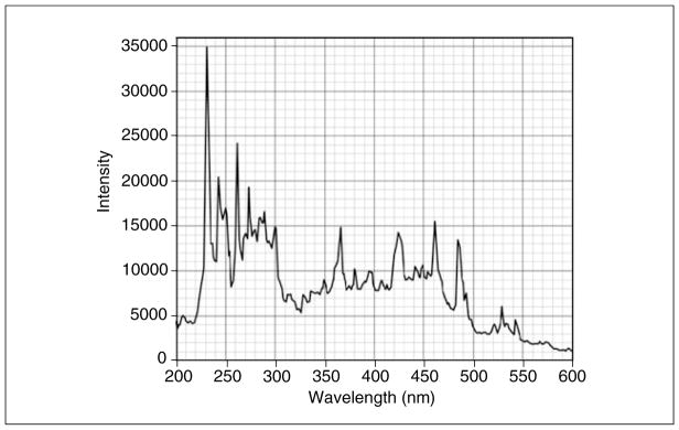
Emission intensity profile of the Xenon flash lamp. A well-tuned instrument will produce an intensity maximum at 230 nm of 15,000 counts or higher.

The UV-visible detector can be used for both absorbance and intensity experiments. In intensity mode, the intensity of the light passing through each channel is independently recorded, without any reference subtraction (Kar et al., 2000). Conversion of intensity data to pseudo-absorbance data requires a reliable reference intensity, which can be obtained by simultaneously scanning one channel filled with water only. Any intensity fluctuations in the lamp occurring over time (e.g., through slow formation of a deposit on the lamp window) are precisely recorded by also measuring the water channel at each scan cycle. UltraScan will use this information to convert the intensity data to pseudo-absorbance data by applying the conversion shown in Equation 7.13.4:

$$A=-log\left(\frac{I_S}{I_R}\right)$$ Equation 7.13.4

where I_R is the reference intensity from the water scan, averaged over several radial points, A is the pseudo-absorbance value, and I_S is the intensity value obtained from each channel containing a sample.

There are distinct advantages for using the intensity collection mode for SV experiments in conjunction with UltraScan data analysis, while absorbance mode is recommended for SE experiments. In addition to the fact that all but one channel in an experiment can be used for samples instead of reference solutions, the data quality of intensity scans tends to be higher than that of absorbance scans. To better understand the reason for this difference in data quality, the source of various noise signals merits further discussion. In an absorbance experiment, the light passes through several optical components, starting with the lamp window and the monochromator. Next, the light passes through the upper cell window, the solution column, the lower cell window, the focusing optics, the slit assembly, and finally through the photomultiplier window. Each light flash is independently imaged and collected as a single intensity data point. In an absorbance experiment, each radial position is measured twice, once through the sample sector, and once through the reference sector. Each observed intensity measurement I_obs is convoluted with a number of noise sources, which can be summarized as Equation 7.13.5:

$$I_{\mathit{obs}}=I_0-N_{ri}-N_{ti,\mathit{window}}-N_{ti,\mathit{other}}-N_S-S$$ Equation 7.13.5

where I₀ is the intensity of the lamp, N_ri is the radially invariant noise component, N_ti,window is the time invariant noise component contributed by the windows of the sample cell, N_ti,other is the time invariant noise component contributed by all other optical components, N_s is the stochastic noise component contributed by the flash lamp and electronics, and S is the intensity loss due to absorbance by buffer and analyte. The radially invariant noise contribution arises from changes in lamp intensity over time, or, in the case of interference optics, from slight changes in optical path length due to heating and cooling cycles in the instrument. This noise will add a constant offset to the baseline of each scan. Time-invariant noise contributions arise from imperfections of any optical component where light passes through. For example, a fingerprint on a cell window will not vary over time and produce the same invariant noise contribution to every scan taken. Fortunately, time invariant and radially invariant noise contributions can be removed algebraically with analysis methods implemented in UltraScan (Schuck and Demeler, 1999). While all noise contributions are additive, it is important to note that the time invariant noise contributions from the upper and lower cell window are different for the sample and reference sector (e.g., a scratch on the window may be in a slightly different position on the reference sector than in the sample sector).

While time invariant noise contributions from optical components other than the cell window are effectively removed from the resulting data by virtue of the reference subtraction employed during absorbance data acquisition mode, a small amount of time invariant noise resulting from the difference in cell window noise remains in the data. This is particularly troublesome in cases where very narrow, high-amplitude time invariant noise signals distort the sample signal, such as small scratches on cell windows, because the precision of the radial scanning stepping motor is too low to detect such narrow distortions always at the same radial position. As a consequence, such distortions are reported at different radial values and are no longer truly time invariant. In addition, each radial point from each sector has a unique time-dependent stochastic noise signal associated with itself, which is different for the corresponding radial observations from reference and sample sector. During subtraction of the reference signal from the corresponding sample signal, the stochastic noise contributions and the (random) differences in the time invariant noise signals from the upper and lower windows are convoluted. Whenever stochastic noise signals are convoluted, the total noise signal increases on average by a factor of square root of 2, which is undesirable.

When intensity measurements are taken, all time invariant noise contributions are additive and can be represented in a single time invariant noise signal. For velocity experiments, it is fortunately possible to entirely eliminate the time invariant noise contributions by algebraic means (Schuck and Demeler, 1999), providing a signal-to-noise improvement by a factor of $\sqrt{(2)}$ ratio for intensity SV experiments over absorbance SV experiments. This principle is demonstrated in Figure 7.13.3, which shows a comparison between measurements made of the same sample in both intensity and absorbance mode. Here, a sedimentation velocity experiment was performed first in absorbance mode, and then the same sample was re-sedimented in intensity mode re-using the same cell and run conditions. Figure 7.13.3A shows the data obtained from the absorbance measurement, and Figure 7.13.3B shows the intensity data. On first glance, the intensity data appears to be significantly worse, because the amplitude of the time invariant noise is quite significant. The time-invariant noise contributions for both experiments are compared in Figure 7.13.4. In the absorbance experiment (Fig. 7.13.4A), the majority of the time invariant noise is eliminated through subtraction of the reference channel. The remaining time invariant noise is hence due solely to differences between the cell windows. However, the significant time invariant noise contribution shown in the intensity data (Fig. 7.13.4B) is easily removed by appropriate fitting algorithms in UltraScan, leaving only stochastic noise. Figure 7.13.3C shows the stochastic noise residuals of a data fit using the 2-dimensional spectrum analysis (2DSA) (Brookes et al., 2009) of the absorbance data and Figure 7.13.3D the residuals for the intensity data when analyzed with identical analysis settings. Panels E and F in Figure 7.13.3 show the noise-corrected data obtained from the absorbance and intensity experiments. It is clear to see that the quality of data obtained when measured in intensity mode is significantly better than the quality of data obtained in absorbance mode. This is reflected in the residual mean square deviation (RMSD) of the fit, which differs approximately by a factor of √(2) as predicted by statistical theory (3.5543 × 10⁻³ for absorbance mode, and 2.3705 × 10⁻³ for intensity mode).

Figure 7.13.3.

Data quality comparison between absorbance (A, C, E) and intensity (B, D, F) data: A sedimentation experiment of a solution containing 0.1 OD ovalbumin was scanned at 280 nm in absorbance mode (panel A) and fitted by two-dimensional spectrum analysis with time- and radially invariant noise removal. The residuals of this fit are shown in panel C, and the noise corrected data are shown in panel E. After the experiment, the solution was shaken up and rescanned in intensity mode under identical run conditions, producing corresponding experimental scans in panel B, residuals in panel D and noise-subtracted data in panel F. The increased noise that can be seen in the absorbance experiment is due to the convolution of two stochastic measurements (reference and sample), which amplifies the stochastic noise approximately by a factor of √(2). In this case, the RMSD of the absorbance experiment was 3.5543 × 10⁻³ and the RMSD of the intensity experiment was 2.3705 × 10⁻³. The additional noise seen in panel B arises from time-invariant noise components contributed by optical components other than cell windows, which are subtracted out in the absorbance experiment. Regions in the residuals where deviations exceed the average are due to narrow, high-amplitude time invariant noise signals (most likely scratches on the cell windows) that are poorly reproduced by the scanning optics due to lack of precision in the radial scanning system.

Figure 7.13.4.

Time invariant noise contributions in the absorbance experiment (A) and the intensity experiment (B) shown in Figure 7.13.3. For clarity, the intensity-derived time-invariant noise vector is transposed by −0.2 absorbance units. While the amplitude for the low frequency noise is larger in the intensity measurement, the amplitude of the high frequency noise from the absorbance measurement is larger due to the convolution of the two noise vectors, one from each channel.

Rayleigh Interference Optics

The interference optics measure the refractive index difference between a sample and a reference cell. The pattern of shifted fringes generated by the refractive index differences are converted by a fast Fourier transform into concentration profiles, which can then be evaluated by standard methods. There are several significant advantages with interference optics: first, sedimentation can be performed in the presence of absorbing buffer components. Second, the precision of the interference optical system is about 10-fold higher than that of absorbance optics. Third, the dynamic range of the interference optics is much higher than the dynamic range of the absorbance optics. This makes it ideal for the measurement of more highly concentrated solutions. Finally, the radial and temporal data density is much higher than in the absorbance optics. It should be noted that the sample should not absorb at 675 nm, which is the wavelength of the laser. Data scans can be acquired with less than 10 sec of scanning time, and the radial resolution of the data is more than twice as high as that of absorbance data with a constant radial grid. When performing interference experiments, it is important to note that generally all components dissolved in the solution contribute to the interference pattern, even salts and buffer components. For that reason, some experimentalists choose to run against the buffer in the reference cell, with the menisci from both channels matched as closely as possible. Besides matching the menisci, this requires that the refracting buffer components are present at the same concentration in the reference, as well as the sample channel. A match is best achieved by extensive dialysis and using the dialysate or by using the column eluate from a size elution chromatography experiment as a blank in the reference channel. Alternatively, if analyzing the data with UltraScan, it is possible to simply use purified water in the reference cell. In that case, UltraScan can model the sedimentation of the buffer components in addition to the analyte of interest, and separate the signals of each component. In such a setup, there is no danger from buffer components sedimenting under mismatched menisci, which would distort the results by overlaying an unpredictable difference spectrum of the buffer components on top of the analyte signal. Another point to keep in mind with interference optics is the use of cell windows. Standard quartz windows tend to have a strong refractive index heterogeneity. Furthermore, the refractive index properties seem to change with centrifugal forces acting on the windows. This prevents these noise signals to be treated as pure time-independent signals. Sapphire windows present in many cases a very good alternative, because they do not exhibit strong refractive index heterogeneities. Another complication can occur with improperly focused optics. In order to minimize Wiener skewing effects, the optics should be focused on the 2/3 plane, and steep gradients should be avoided by using a lower rotor speed, and by using longer solution columns.

Fluorescence Optics

The strongest advantage of the fluorescence optics is the superior sensitivity and exquisite selectivity (MacGregor et al., 2004). Some samples can be measured reliably at picomolar concentrations. As in interference optics, the dynamic range is much larger than in absorbance optics; however, the user has to manually adjust gain settings to optimally exploit the dynamic range. A drawback is the inability to look at intrinsic tryptophan fluorescence. Instead, all molecules must be labeled with fluorescent probes whose excitation range coincides with the excitation laser’s wavelength (488 nm). Tags such as Alexa488, SybrGreen (for dsDNA), fluorescein, and other fluorescein-based tags can be used. Proteins can also be engineered to contain a green or yellow fluorescent protein tag, providing intrinsic fluorescence. Emission intensity is filtered to only allow signals above 500 nm to be observed. Samples must be degassed prior to analysis and the addition of a nontagged carrier protein such as ovalbumin at a concentration of 0.1 mg/ml is recommended, especially for samples with proteins at very low concentration. The great selectivity in fluorescence optics permits the analysis of intrinsically labeled proteins without purification in whole cell extract suspensions, or in blood serum (Kingsbury et al., 2008; Kroe and Laue, 2009), or other physiological solutions.

EXPERIMENTAL DESIGN

Proper experimental design is a crucial step in a successful SV or SE experiment, and attention needs to be paid not only to the run conditions, but also to the condition of the instrument. A series of instrument diagnostics and sample preparation steps will help to obtain optimal data for analysis.

Instrument Diagnostics

A successful experiment clearly depends on a properly calibrated and well functioning instrument. The Beckman XL-A/I instruments do require periodic maintenance and calibration. The following tests should be performed to ensure the instrument is in optimal condition. For all detectors, a careful calibration of the optical focus is essential. This should be performed by Beckman service. The user can regularly perform several other diagnostics, among them is the radial calibration of the instrument. Guidelines for these procedures are available in the instrument manual. For absorbance optics, the intensity of the lamp should be routinely checked. A wavelength intensity scan of an empty rotor hole performed at 6.5 cm should produce an intensity pattern shown in Figure 7.13.2. An intensity scan across an empty rotor hole at 230 nm from 5.9 cm to 7.1 cm should produce a pattern that does not vary more than 10% across the cell. If the intensity at 230 nm is low, or varies more than 10%, either the lamp needs to be cleaned or the slit assembly and focusing optics need to be serviced. Sometimes, rotating the lamp to a different angle also helps. Reproducibility of the wavelength should be within ±1 nm, several wavelength intensity scans should produce plots that show congruent emission peaks at all wavelengths. Another issue that frequently needs to be checked with the XL-A optics is the radial reproducibility. In some cases, dirt, oil, and other contaminants can impede the smooth operation of the slit assembly, and cause irregular radial positioning. This problem is easily detected when the meniscus position of a high-speed absorbance experiment varies from scan to scan. This problem is corrected by thoroughly cleaning the slit assembly.

Sample Preparation and Sample Concentration

The flexibility introduced by a choice of several optical detectors permits the analysis of proteins under a very large range of analyte concentration, buffer pH, and ionic strength, and in the presence of detergents, nucleotides, reductants, and other additives. In general, the most reliable results are obtained by analyzing the samples under dilute conditions, which minimize concentration-dependent hydrodynamic and thermodynamic non-ideality. Protein concentrations of less than 1.0 optical density units at 230 nm are generally dilute enough to produce negligible concentration-dependent non-ideality contributions. Use of wavelengths below 250 nm excludes the use of many additives and virtually all reductants (see Fig. 7.13.1). If in doubt, the absorbance spectrum of the additive should be measured against water, to adjust the concentration of the additive such that the total optical density does not exceed the dynamic range. It often helps to have some salt present in the buffer (20 to 50 mM) to reduce the effect of charges on the protein, which may contribute to concentration-dependent non-ideality. Another issue to be aware of includes the presence of gradient-forming buffer components. In principle, molecules as small as a few hundred Daltons (such as salts) can produce density and viscosity gradients at higher speeds, which will affect the sedimentation and diffusion coefficients over the length of the column. Reducing the speed, or lowering the concentration of the gradient-forming component will reduce the gradient to negligible levels. If in doubt, a velocity experiment can be performed with the buffer solution measured at the desired speed against water using interference optics. This experiment will reveal the approach to equilibrium gradient as a concentration profile of the buffer components, from which the density and viscosity differences at the top and at the bottom of the cell can be estimated. These values can be entered into the UltraScan hydrodynamic parameter simulation routine and the effect on the change in s and D can be estimated. The condition of the centerpieces is very important; they should be free of scratches, which can cause turbulences and convection of the solutes, and the use of scratch-free windows is recommended. A proper alignment of the cell in the rotor hole is critical. Misaligned cells also cause turbulences and convection, which distort the sedimentation profiles. Proper alignment within 0.1 degrees can be achieved with a commercially available cell alignment tool (http://www.spinanalytical.com/). For the same reason, worn-out cell housings and loose fitting centerpieces should not be used. For velocity experiments, intensity experiments can take advantage of the reference channel, which can be used for low concentration samples (<0.5 OD to avoid inadvertent resetting of the photomultiplier tube gain setting). No such restrictions exist for the sample channel. It is therefore recommended to run the same sample at multiple concentrations, ranging from 0.1 to 1.0 OD. By taking advantage of the reference channels, up to 5 samples can be measured simultaneously in a 4-hole rotor, or 13 samples in an 8-hole rotor with no additional scanning time compared to absorbance scans. In intensity measurements, one of the channels should always be reserved for a water reference.

An important application for SE experiments is the measurement of equilibrium constants for self-associating systems. In dynamic reactions like monomer-polymer oligomerizations, the most reliable answers are obtained when a broad concentration range can be analyzed that contributes sufficient signal from monomer, as well as the oligomeric forms. Due to mass-action laws, the monomer species will be emphasized at low concentrations, while the signal from the oligomer will be predominant at high concentrations. A global analysis over several concentrations will therefore provide the most reliable result. Measurement at different wavelengths will contribute further to the broadening of the concentration range. Ideally, measurements of loading concentrations at 0.3, 0.5, and 0.7 OD at 215 nm and 230 nm (buffer system permitting), and at 280 nm, and in interference mode should be combined in a global fit to optimize the signal from both monomer and oligomeric species. 6-channel centerpieces can be used to accommodate three concentrations per cell. A simple test that should always be performed first is to perform a velocity experiment of the same sample at three different concentrations. Not only will this run confirm that the sample is pure enough for equilibrium analysis and does not contain any aggregates or contaminants, but it will also identify the presence of reversible association by comparison of the sedimentation coefficient distributions from each concentration. If these concentrations overlay, the sample is non-interacting, or outside the equilibrium constant concentration (Demeler et al., 1997). For SE experiments, the intensity mode is not appropriate, and absorbance mode must be used. This requires the use of a reference solution, which should always be water, except in interference mode where meniscus-matched buffer solution should be used.

Speed Selection

Rotor speed plays an important role in the experimental design, and several factors need to be balanced. A high rotor speed in a SV experiment produces the best resolution when performing composition analysis, and when the accuracy of sedimentation coefficients and partial concentrations is critical. However, at high rotor speed all solutes will sediment rather quickly with little time to diffuse. This will reduce the signal observed for the diffusion coefficient, which provides frictional information critical for shape and molecular weight calculations. To obtain the best signal for both sedimentation and diffusion coefficients, UltraScan offers global fitting of multi-speed experiments, which combine the strong diffusion signal from the slow experiment with the strong sedimentation and partial concentration signal from the high-speed experiment into a single solution (Brookes et al., 2009). From such globally fitted data, molecular weight or partial specific volume can be obtained, provided one or the other is known a priori. For single speed SV experiments, the speed should be chosen to be a good compromise between high and low speed sedimentation. This can best be achieved by modeling the solutes in the “Finite Element Simulation (ASTFEM)” implemented in UltraScan. A speed should be selected that results in a minimum of 40 to 60 scans that result in complete pelleting of the solute. For experiments involving multiple cells, the scanning time of each cell needs to be taken into account when selecting the proper speed. In SE experiments, high speed increases the curvature of the concentration gradient. If the speed is too high, a large portion of the data points correspond to a meniscus-depleted baseline, and only a few data points show any measurable absorbance. Moreover, if the speed is too high, the gradient at the bottom of the cell is too steep to provide useful signal for any optical detector. On the other extreme, if the speed is too low, the gradient of the experiment is too shallow, and it will not contain much useful information. Ideally, the profiles of 4 to 5 intermediate speeds should be collected and globally fitted using the Nonlin procedure (Johnson et al., 1981) implemented in the UltraScan software. The appropriate speeds depend on the molecular weight of the solute and the density of the solution, and are calculated by the UltraScan equilibrium time simulation module. The speeds should be chosen such that the reduced effective molecular weight, σ (Eqn. 7.13.6; see Yphantis, 1964), ranges between 1 to 6.

$$\mathrm{\sigma }=\frac{M{\mathrm{\omega }}^2(1-\overline{\mathrm{\nu }}\mathrm{\rho })}{RT}$$ Equation 7.13.6

Loading Volume and Column Height

For SV experiments, it is advantageous to maximize the column height in order to increase the information content of the data. A longer column produces more data points and improves the fitting statistics of the experiment. A loading volume of 450 μl is recommended for all velocity experiments. When using the interference optics, the air-to-air region should be scanned; it is required for the baseline alignment of all scans (Schuck and Demeler, 1999). For SE experiments, the time required for attaining equilibrium is proportional to the height of the solution column. Therefore, a compromise between the number of data points for fitting and the length of time required to reach equilibrium needs to be found. Typically, a 3- to 3.5-mm column is sufficient, requiring about 100 to 120 μl loading volume.

Data Acquisition and Instrument Settings

Since SE experiments should be measured at multiple concentrations, the experimental setup is ideal for the measurement of intrinsic extinction profiles. The precise knowledge of extinction coefficients at different wavelengths is required for accurate fitting of reversible reaction models. Therefore, at the beginning of each experiment, each concentration of the same sample should be wavelength-scanned in order to contribute several absorbance profiles, each at a different concentration range. The radial position for the wavelength scan should be the center of the solution column. These profiles can later be globally fitted with the Ultrascan “Global Extinction Fit” to a sum of Gaussian terms to provide an intrinsic extinction profile (see Fig. 7.13.5). In SE experiments, the UltraScan “Equilibrium Time Prediction” module will accurately predict how long a particular sample will take to reach equilibrium at a given speed, buffer viscosity, column height, and column position. The output of this module should be used to program the “Methods Scan” option from the Beckman Data Acquisition software. This module should be programmed to acquire one scan at the equilibrium time from each concentration at the optimal wavelength with 20 to 30 averages in step mode and with the highest radial resolution setting possible (for the absorbance optics the smallest step size is 0.001 cm). The method should allow sufficient time for scanning to complete before accelerating to the next speed. In the end, one equilibrium scan for each loading concentration and speed should be available that was taken at the highest radial resolution setting possible. For velocity experiments, all measurements performed with the UV/visible detector should be measured in intensity mode. The scanning time should be as rapid as possible, and continue until all material has either pelleted or reached equilibrium. In no case should data acquisition be aborted until the boundary has moved to the bottom of the cell. Radial settings should be at 0.003 cm and should be measured in continuous mode with 0 sec delay between successive scans. When using the absorbance optics, a radial absorbance scan recorded at 3000 rpm can be used to set the minimal and maximal radius. Avoiding the scanning of unnecessary data points shortens the time required for each scan, providing additional scans of the data region of interest. Unlike equilibrium experiments, the wavelength setting should never be changed during a velocity experiments. The reason is the lack of precision of the monochromator to reset to the selected wavelength. Even small changes occurring during resetting of the wavelength can cause major changes in extinction, especially at wavelengths near the absorbance shoulder (e.g., 230 nm in proteins). In SE experiments, this is not an issue because UltraScan contains features that can correct for the inconsistency in wavelengths by means of the intrinsic extinction profile determined from the wavelength scans that were acquired beforehand.

Figure 7.13.5.

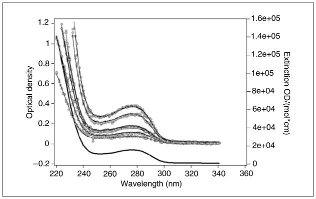
Global extinction fit (thin black lines) of 15 wavelength scans (gray circles) at five different loading concentrations. Each loading concentration is scanned three times with 1-nm increments and fitted globally to the same sum of Gaussian terms to represent the intrinsic extinction profile with the UltraScan “Global Extinction Fit” module. Each loading concentration is represented by the same Gaussian sum, but with a different amplitude. The intrinsic extinction profile (heavy black line) of the protein is normalized by a known extinction coefficient (typically at 280 nm).

Choosing Between SV or SE Experiments

In general, SV experiments are well suited for characterizing any sample for composition, molecular weight, and shape distributions, and partial concentrations. New analysis methods developed in UltraScan for the analysis of SV experiments also provide the ability to characterize reversible reactions, including the determination of equilibrium constants and kinetic rate constants (Demeler et al., 2010). SV experiments and high-resolution methods implemented in UltraScan are also the method of choice for the characterization of sample purity and presence of aggregates or contaminants. While equilibrium analysis has long been the gold standard for assessing solute molecular weight, due to the shorter run time, much larger solution column, and the larger number of scans, the increased data density can more fully describe the data. In addition, much of the information traditionally measured in SE experiments with long run times can now be acquired at higher precision with SV experiment in a much shorter run time. Nonetheless, SE experiments can still provide a fairly reliable average molecular weight spectrum, and determine quite reliably the equilibrium constants for very pure 2-component, maximally 3-component systems. When equilibrium constants need to be known accurately, a confirmation of the SV results with a SE experiment are well advised. Whenever the sample is prone to aggregation, is less than 95% pure, or chemically unstable, the results from SE experiments will have little or no value.

TIPS FOR DATA ANALYSIS

The following steps highlight the recommended approach for obtaining optimal data analysis results.

SV Experiments

After collection of multi-speed velocity data, each intensity dataset is separately analyzed by the dc/dt approach (Stafford, 1992) implemented in UltraScan to identify the s-value range that needs to be fitted. This method effectively removes the time-invariant contributions present in intensity data and provides model independent s-value distributions. Due to the lack of diffusion deconvolution, the dc/dt distributions tend to overestimate the actual s-range, but this is acceptable, while an underestimation of the s-value range will result in serious error. Subsequent analysis methods will automatically discard s-values that are not present in the data. The dc/dt estimate is used to set the s-value range for the 2-dimensional spectrum analysis (2DSA) (Brookes et al., 2009), the next step in the analysis. The frictional ratio range should be set to 1–4, and can be extended if the sample is known to contain molecules with very extended shapes, such as fibrillar aggregates or long, linear DNA molecules. This analysis is performed on a supercomputer with a 10 × 10 grid setting, and typically 20 to 25 grid repetitions, or less, if the s-value range is very small. Time-invariant noise correction should be turned on during this first step, as should be the iterative optimization approach with at least 3 to 5 iterations. Also recommended is the fitting of the meniscus position. A range of 0.01 to 0.03 cm with 7 to 15 data points is recommended. The resulting RMSD values are then plotted against the meniscus position and fitted to a 2nd order or 3rd order polynomial. The optimal meniscus position can be obtained by setting the first derivative of the fitting function equal to zero and solving for the radius (see Fig. 7.13.6). After subtracting the time invariant noise obtained in the initial fit, radially invariant noise can also be removed by refitting the data. If the obtained s-value distribution appears broad or continuous with many discrete species, a further improvement can be obtained by performing a 30 to 50 iteration Monte Carlo analysis, which will reduce the impact of stochastic noise on the obtained solution (Demeler and Brookes, 2008) and emphasize the solute contributions. If the 2DSA solution suggests the presence of only a few, discrete solutes, a parsimonious regularization by genetic algorithm (GA) analysis of the 2DSA distribution is well advised (Brookes and Demeler, 2007). This method will remove false-positive solutes (caused by noise present in the data) from the distribution and refine the 2DSA solution by highlighting only essential components present in the solution. This approach can further be refined by also performing a 30 to 50 iteration Monte Carlo analysis in conjunction with the GA analysis. If multiple speeds and concentrations were measured, a van Holde-Weischet analysis should be performed on each sample (Demeler and van Holde, 2004), and the s-value distributions should be overlaid for comparison. If the distributions suggest little change for the multiple conditions, further accuracy can be obtained by combining multiple speeds and multiple concentrations into a global 2DSA or GA fit. If concentration-dependent changes are apparent, the distributions should be evaluated to determine if reversible oligomerizations appear to be present. In such a case, a nonlinear model can be used to fit the data to models describing user-defined reversibly reacting systems (Cao and Demeler, 2008; Demeler et al., 2010) with the GA optimization method. For pure systems containing only oligomeric species, a molecular weight constrained 2DSA or GA analysis can be performed, constraining the solution to an approximate non-interacting model where only selected oligomeric forms presumed to be present in the solution are described.

Figure 7.13.6.

Meniscus fit from RMSD values obtained in multiple iterations of 2DSA analysis fits. Such iterations always result in well-conditioned error surfaces that are easily fit by second-or third-order polynomials as shown here. The minimum occurs at the position where the first derivative of the polynomial is equal to zero.

SE Experiments

In a first analysis, all scans from the SE experiment should be globally evaluated with a fixed molecular weight distribution model. This model fits the data to a sum of noninteracting molecular weight species, and provides a molecular weight histogram for all species in the system. Typically, 100 molecular weight species are sufficient to be fitted over the molecular weight range thought to be represented in the experimental data. The correct fitting range can be determined easily by trial and error by simply repeating the fit with several range limits. If the RMSD no longer changes to a lower value, the range is sufficiently covering the solutes present in the sample. The molecular weight histogram can often be improved in clarity by further performing a Monte Carlo analysis on this model. This fit serves two purposes: due to the degeneracy of the model (100 species are fit), this model will produce the lowest possible RMSD value for the any dataset. Secondly, it will provide an overview of the molecular weight range of the species in the sample. This often helps to identify more restrictive models, and with the choice of additional constraints. The RMSD values obtained by fitting with any subsequent model should then be compared to the “gold standard RMSD” from the fixed molecular weight distribution model. In evaluating which model best represents the given data, it is important to note that the RMSD is inversely correlated to the number of fitting parameters, and the number of fitting parameters is inversely correlated to the confidence one can have in any particular parameter. In other words, if the RMSD does not change significantly when changing the model from a more constraint model to a less constraint model, then the parameters of the more highly constrained model provide the highest significance. What exactly constitutes “significance” is best evaluated with statistical tests based on Monte Carlo analysis implemented in UltraScan. These methods provide 95% and 99% confidence intervals for each parameter fitted in a model, which will help the experimentalist to determine the most likely model. The most constrained model is the model with the fewest parameters. For models provided in UltraScan, the order from most constrained to least constrained is: (1) single ideal species, (2) monomer-n-mer, (3) monomer-n-mer-m-mer, (4) two component ideal species, non-interacting, and (5) fixed molecular weight distribution. The number of fitted parameters is listed in the nonlinear least squares fitting panel of UltraScan for each model.

A comprehensive instrument guide describing cell assembly, instrument operation and diagnostics, as well as a maintenance guide is available for download from the AUC manual wiki (Schirf and Planken, 2008).

DATA MANAGEMENT

The UltraScan software includes a database back end that provides convenient tools to support multi-user facilities and to track projects from multiple investigators. This system is used to manage experimental data, analysis results, and to store supporting information such as buffer composition, protein and nucleic acid sequences, gel images, and absorbance spectra, as well as other ancillary information, which are associated with the experimental data. The stored protein sequences are then used to automatically estimate molecular weight, partial specific volume, and extinction coefficients at 280 nm, and the buffer composition information is used to calculate buffer density and viscosity. This system is collectively called the UltraScan Laboratory Information Management System (USLIMS) and can be accessed both through UltraScan and through a Web portal offered by the Teragrid Science Gateway (http://www.teragrid.org/gateways/gateway_list.php). The Teragrid Science Gateway portal also is used to submit analysis jobs to NSF Teragrid supercomputers, which manage the compute-intensive analysis methods offered by UltraScan (Brookes and Demeler, 2008). Results are stored in the database and conveniently organized as Web pages, which can be accessed by the data owners and authorized collaborators.

CHECKLISTS

Experimental Design and Data Collection Protocol

1. Before starting the AU experiment, perform recommended diagnostic procedures and confirm that the instrument is in optimal operating condition (see Instrument Diagnostics).

2. Previously uncharacterized samples should always first be measured by SV. The most appropriate speed can be selected by first simulating the experiment with the UltraScan ASTFEM simulation module using prior knowledge about the sample (molecular weight, assembly state, etc.). The speed should be chosen such that a minimum of 30 to 40 scans spanning the entire cell can be collected from each channel. A high speed is preferred for the initial experiment since it emphasizes resolution and more clearly identifies the presence of aggregates and sample heterogeneity.

3. To confirm reversible self-association, multiple concentrations should be measured. Three concentrations at 0.3, 0.6, and 0.9 OD at 230 nm at 450 μl each in a transparent buffer system with a moderate amount of salt (20 to 50 mM) should be used as a first test (see Absorbance optics). Place the 0.3 OD sample in the reference channel, and the 0.6 OD sample in the corresponding sample channel of the same cell. The 0.9 OD sample should be placed in a separate cell and should be measured against water. The water channel will serve as a reference for the entire experiment. Interference or fluorescence detection can be used to further extend the concentration range. See the Experimental Design section for additional details regarding sample preparation.

4. For samples containing absorbing buffer components, interference optics can be used instead, or the wavelength can be adjusted to optimize sample extinction while minimizing buffer absorption. See the Background section above for a discussion on the selection of optical systems.

5. Precool the rotor and wait for the temperature to stabilize before accelerating the rotor to the final velocity speed. As soon as the selected speed has been reached, start to collect scans until the sample is either at equilibrium or pelleted. Collect data without time delay between scans, as fast as the machine can collect. Excessive or unnecessary scans can be deleted later on.

6. If the equilibrium constant is of interest, the concentration should be chosen such that both monomer and oligomeric species are sufficiently abundant in order to obtain enough signal from all species. Multiple experiments at different wavelengths or optical systems may be required to find the optimal concentration range.

EXPERIMENTAL ANALYSIS FLOWCHART

1. If an intensity experiment has been performed, convert the intensity data to pseudo-absorbance data. Use the water channel measurement as a reference intensity for each scan. This can be accomplished with the UltraScan intensity data conversion module.

2. Edit the velocity data with the UltraScan editor for the optical system chosen. For interference data, a radial invariant noise component may be eliminated during editing. Estimate the s-value range using the dc/dt method (Stafford, 1992) as implemented in UltraScan for data containing strong time-invariant noise components, or using the enhanced van Holde–Weischet analysis (Demeler and van Holde, 2004) for data mostly free of time-invariant noise. Commit to the USLIMS database.

3. Perform a 2DSA (Brookes et al., 2009), fitting time invariant noise and optionally also the meniscus with 7 to 15 points over a 0.03 cm range. Use the s-value range estimated in the previous step, and set the frictional ratio to range between 1 and 3 for protein samples, and 1 to 6 for linear DNA fragments and samples that form elongated aggregates or fibrils.

4. Subtract time-invariant noise from the data, and edit the meniscus position (see SV experiments). Update the edited data in the database.

5. Optionally, repeat the 2DSA by simultaneously fitting for time invariant and radially invariant noise. Subtract both time and radially invariant noise vectors. For interference data, or data with significant radial invariant noise contributions, the analysis should be repeated with radial-invariant noise correction turned on. Afterwards, the radial-invariant noise contributions should be subtracted as well and the edited data should be updated in the database.

6. Using the enhanced van Holde-Weischet analysis (Demeler and van Holde, 2004), a more precise sedimentation coefficient range can now be determined. An overlay of the three integral distribution plots from each concentration will further reveal association properties and permit a comparison in sample composition (see Demeler et al., 1997 for a discussion of van Holde-Weischet result interpretation).

7. Additional refinement of the results can be achieved by performing a 2DSA combined with a Monte Carlo analysis. This approach will improve the signal-to-noise ratio and attenuate the contributions from the remaining stochastic noise.

8. The results from steps 6 to 7 should now be evaluated to decide on possible additional refinement and further analysis. The following outcomes are common, and can be discerned easily from a velocity experiment:

   1. The sample is homogeneous (see Fig. 7.13.7).

   2. The sample is pauci-disperse, with no more than four or five discrete species. A change in concentration has no apparent effect on the sedimentation coefficient distributions. See Brookes and Demeler (2008) and Brookes et al. (2009) for a detailed discussion of the analysis of such systems.

   3. The sample displays clear concentration-dependent, reversible association properties (see Fig. 7.13.8, Fig. 7.13.9, and Table 7.13.1).

   4. The sample is very heterogeneous and displays a broad sedimentation distribution.

   5. The sample is mostly homogeneous, but also contains a small amount of irreversible aggregate or a small molecular weight contaminant or degradation product. Changing the loading concentration does not affect the sedimentation coefficient distribution or relative composition.

9. Based on the outcome, additional questions can be answered by further analysis. For condition 8a, 8b, or 8e, a subsequent genetic algorithm analysis is appropriate. The 2DSA analysis results are used to initialize a genetic algorithm analysis to perform a parsimonious regularization on the samples (Brookes and Demeler, 2007). This will reduce the number of solutes to the essential solutes that describe the data equally well as the 2DSA solution. The genetic algorithm analysis can then be refined by another Monte Carlo analysis in order to enhance the signal-to-noise ratio, and to determine the confidence intervals of the solute parameters. This approach is valid for non-interacting systems and it will result in molecular weights, partial concentrations, and relative shape information for each detected solute. For cases where the sample is monodisperse (see 8a; also see Fig. 7.13.7), an equilibrium experiment can be used to further confirm the molecular weight of the sample. For pauci-disperse samples, the resolution of an equilibrium experiment is generally not sufficient to identify more than one or two non-interacting solutes.

10. If a reversibly associating system is observed (see 8c; also see Fig. 7.13.8), the 2DSA and genetic algorithm Monte Carlo analyses can yield valuable clues about the identity of the oligomeric species and the association properties by providing molecular weights and relative composition. It should be noted that these methods are modeling non-interacting systems. If the system is reversibly self- or hetero-associating, these methods will only approximate the true composition, and the reversible reaction boundary will usually not reproduce the exact values for the monomer and oligomeric species (see Fig. 7.13.9). However, the information from these analyses together with the results from the van Holde-Weischet analysis generally provide unambiguous clues about the type of association that needs to be modeled, and the results can then be used to formulate a possible reaction model and initialize the parameters for a reacting model. Parameter optimization for nonlinear reaction models is best accomplished with the genetic algorithm analysis performed in conjunction with a Monte Carlo analysis. The parameter distributions obtained in this fashion provide important clues to the most likely parameter ranges, especially for frictional ratios, equilibrium constants, and kinetic rate constants of the reaction, which are otherwise difficult to obtain. If several models are plausible, each should be checked for compatibility with the experimental data. The best model should be chosen based on the randomness of the residuals and the overall residual mean square deviation (RMSD). If the system turns out to be a simple, two-component monomer-oligomer system, an optional equilibrium experiment can be used to further confirm the oligomeric status and to provide an independent measurement of the equilibrium constant. In Table 7.13.1 the nonlinear fit by genetic algorithm-Monte Carlo analysis of the same data presented in Figures 7.13.8 and 7.13.9 is shown. As can be seen, the obtained parameters are quite close to the simulated values.

11. For cases where the analysis results in broad, very heterogeneous sedimentation coefficient distributions (8d), the resolution of individual components may be compromised by the heterogeneity. In such a case, the genetic algorithm optimization is not very useful since a parsimonious regularization is not indicated. Instead, further purification and fractionation of the sample may be desirable.

12. For most systems, additional precision can be obtained by performing a global, multi-speed velocity analysis (Brookes et al., 2009). While high-speed experiments emphasize the signal for sedimentation coefficients and composition, a low-speed experiment will allow all samples to diffuse long enough before pelleting to provide additional signal on the diffusion coefficient. Since molecular weight determinations rely on knowledge of both the sedimentation and the diffusion coefficient (see Eqn. 7.13.1), the combined fit of a low-speed and a high-speed experiment also provides enhanced information about molecular weight and shape of the solute(s).

13. When accuracy of the composition analysis is critical (for example, when purity of a drug formulation needs to be determined), a global fit over multiple high-speed experiments is indicated in order to best identify the partial contributions of low-concentration contaminants or aggregates. Such analyses should also be performed in conjunction with Monte Carlo analysis to maximize the statistical certainty of the observations.

Figure 7.13.7.

van Holde-Weischet integral distribution plots for the ovalbumin sample shown in Figure 7.13.3, measured at three different loading concentrations. Filled squares represent 0.1 OD at 280 nm, open circles represent 0.3 OD at 280 nm, and filled triangles represent 0.9 OD at 280 nm. The vertical shape of the s-value distribution indicates homogeneity. Identical results for all three concentrations indicate absence of reversible self-association in this concentration range (in contrast to the data shown in Fig. 7.13.8).

Figure 7.13.8.

van Holde-Weischet integral distribution plots for an ASTFEM simulated velocity experiment of a reversibly self-associating monomer-dimer system with monomer molecular weight of 20 kDa and a frictional ratio of 1.25, equilibrium constant of 1.0, and k_off rate of 0.001/sec. Measured at three different loading concentrations covering a 100-fold concentration range, centered on the equilibrium constant [0.1 (filled triangle), 1.0 (open circles), and 10.0 (filled squares), arbitrary concentration units]. The off-vertical shape of the s-value distribution indicates heterogeneity, the shift in s-value with increasing concentration indicates that this system is reversibly self-associating (in contrast to the data shown in Fig. 7.13.7).

Figure 7.13.9.

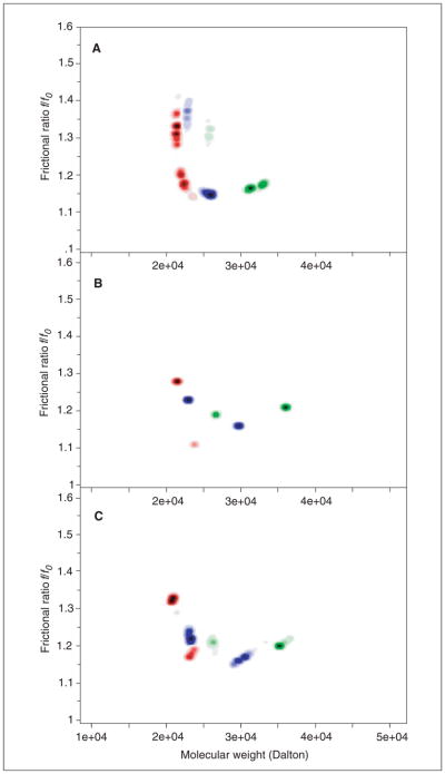
UltraScan composition analysis of the data shown in Figure 7.13.8 (Relative concentrations: red: 0.1, blue: 1.0, green: 10.0). Solute signal is indicated by darkness of color in the 2-dimensional molecular weight/shape plane. (A) Monte Carlo analysis of the 2-dimensional spectrum analysis. (B) Parsimonious regularization by genetic algorithm analysis. (C) Monte Carlo analysis of genetic algorithm analysis shown in (B). The shift to higher molecular weight with increasing concentration is clearly apparent in all three methods. The spreading of peaks is dependent on stochastic noise in the data and is proportional to the confidence intervals of the parameters. Note that a noninteracting analysis does not reproduce the solutes (monomer and dimer) exactly, due to interactions between the oligomeric species. This results in measurements of the weight-average sedimentation coefficient and the gradient-average diffusion coefficient present at each point in the moving boundary. In the extreme of a very slowly interacting system, kinetic effects are minimal and the oligomeric species can be resolved reliably (Brookes et al., 2009). For the color version of this figure go to http://www.currentprotocols.com/protocol/ps0713.

Table 7.13.1.

Fitting parameters for data presented in Figures 7.13.8 and 7.13.9 when fitted with genetic algorithm-Monte Carlo analysis to a reversible self-association model for a monomer-dimer system^a

Parameter	Measured value	95% Confidence interval	Target value
Monomer molecular weight	19.76 kDa	18.46 kDa, 21.06 kDa	20 kDa
Monomer frictional ratio	1.23	1.19, 1.27	1.25
Dimer frictional ratio	1.21	1.17, 1.25	1.25
Association constant	0.877	0.622, 1.133	1.0
koff rate	0.00228/sec	0.00034/sec, 0.0042/sec	0.001/sec

^aUnlike in an SE experiment, the SV experiment not only provides a reliable equilibrium constant, but also provides kinetic information, as well as shape information for all species. These data were simulated with realistic noise, and the variance is reflected in the 95% confidence intervals derived from the Monte Carlo analysis.

CONCLUSION

Analytical ultracentrifugation is a powerful technique for measuring recombinant proteins and other macromolecules in solution. Sedimentation velocity experiments can be used to compare many hydrodynamic, thermodynamic, and molecular parameters between mutants and wild-type and allow the experimentalist to follow changes in equilibrium constants, rate constants, conformation, and composition. A careful experimental design and judicious application of the appropriate optical system and data analysis procedure is critical for a successful experiment, as are the necessary diagnostics to assure reliable instrument operation. The general and model independent fitting methods implemented in UltraScan provide a maximum in resolution and flexibility, while at the same time taking much of the guesswork out of AU data interpretation.

LITERATURE CITED

- Bhattacharyya SK, Maciejewska P, Börger L, Stadler M, Gülsün AM, Cicek HB, Cölfen H. Development of fast fiber based UV-Vis multiwavelength detector for an ultracentrifuge. Prog Colloid Polym Sci. 2006;131:9–22. [Google Scholar]
- Brookes E, Demeler B. Parsimonious regularization using genetic algorithms applied to the analysis of analytical ultracentrifugation experiments. GECCO Proceedings ACM. 2007:361–368. [Google Scholar]
- Brookes E, Demeler B. Parallel computational techniques for the analysis of sedimentation velocity experiments in UltraScan. Prog Colloid Polym Sci. 2008;286:138–148. [Google Scholar]
- Brookes E, Cao W, Demeler B. A two-dimensional spectrum analysis for sedimentation velocity experiments of mixtures with heterogeneity in molecular weight and shape. Eur Biophys J. 2009 doi: 10.1007/s00249-009-0413-5. In press. [DOI] [PMC free article] [PubMed] [Google Scholar]
- Cao W, Demeler B. Modeling analytical ultracentrifugation experiments with an adaptive space-time finite element solution of the Lamm equation. Biophys J. 2005;89:1589–1602. doi: 10.1529/biophysj.105.061135. [DOI] [PMC free article] [PubMed] [Google Scholar]
- Cao W, Demeler B. Modeling analytical ultracentrifugation experiments with an adaptive space-time finite element solution for multi-component reacting systems. Biophys J. 2008;95:54–65. doi: 10.1529/biophysj.107.123950. [DOI] [PMC free article] [PubMed] [Google Scholar]
- Cölfen H, Laue TM, Wohlleben W, Schilling K, Karabudak E, Langhorst BW, Brookes E, Dubbs B, Zollars D, Rocco M, Demeler B. The Open AUC Project. Eur Biophys J. 2009 doi: 10.1007/s00249-009-0438-9. In press. [DOI] [PMC free article] [PubMed] [Google Scholar]
- Demeler B. UltraScan-a comprehensive data analysis software package for analytical ultracentrifugation experiments. In: Scott DJ, Harding SE, Rowe AJ, editors. Modern Analytical Ultracentrifugation: Techniques and Methods. Royal Society of Chemistry; London: 2005. pp. 210–229. [Google Scholar]
- Demeler B. UltraScan Version 9.9 - A multi-platform analytical ultracentrifugation data analysis software package. 2009 http://www.ultrascan.uthscsa.edu.
- Demeler B, van Holde KE. Sedimentation velocity analysis of highly heterogeneous systems. Anal Biochem. 2004;335:279–288. doi: 10.1016/j.ab.2004.08.039. [DOI] [PubMed] [Google Scholar]
- Demeler B, Brookes E. Monte Carlo analysis of sedimentation experiments. Prog Colloid Polym Sci. 2008;286:129–137. [Google Scholar]
- Demeler B, Saber H, Hansen JC. Identification and interpretation of complexity in sedimentation velocity boundaries. Biophys J. 1997;72:397–407. doi: 10.1016/S0006-3495(97)78680-6. [DOI] [PMC free article] [PubMed] [Google Scholar]
- Demeler B, Brookes E, Wang R, Shirf V, Kim CA. Characterization of reversible associations by sedimentation velocity with UltraScan. Macromol Biosci. 2010 doi: 10.1002/mabi.200900481. In press. [DOI] [PMC free article] [PubMed] [Google Scholar]
- Giebeler R. The Optima XL-A: A new analytical ultracentrifuge with a novel precision absorption optical system. In: Harding SE, Rowe AJ, Horton JC, editors. Analytical Ultracentrifugation in Biochemistry and Polymer Science. Royal Society of Chemistry; Cambridge: 1992. pp. 16–25. [Google Scholar]
- Johnson ML, Correia JJ, Yphantis DA, Halvorson HR. Analysis of data from the analytical ultracentrifuge by nonlinear least squares techniques. Biophys J. 1981;36:575–588. doi: 10.1016/S0006-3495(81)84753-4. [DOI] [PMC free article] [PubMed] [Google Scholar]
- Kar SR, Kingsbury JS, Lewis MS, Laue TM, Schuck P. Analysis of transport experiments using pseudo-absorbance data. Anal Biochem. 2000;285:135–142. doi: 10.1006/abio.2000.4748. [DOI] [PubMed] [Google Scholar]
- Kingsbury JS, Klimtchuk ES, Laue TM, Théberge R, Costello CE, Connors LH. The modulation of transthyretin tetramer stability by cysteine-10 adducts and the drug diflunisal: Direct analysis by fluorescence-detected analytical ultracentrifugation. J Biol Chem. 2008;283:11887–11896. doi: 10.1074/jbc.M709638200. [DOI] [PMC free article] [PubMed] [Google Scholar]
- Kroe RR, Laue TM. NUTS and BOLTS: Applications of fluorescence detected sedimentation. Anal Biochem. 2009 doi: 10.1016/j.ab.2008.11.033. In press. [DOI] [PMC free article] [PubMed] [Google Scholar]
- Kumar D. Absorbance spectra for common buffer systems. 2006 http://uslims.uthscsa.edu/cauma/buffer2.php.
- Lamm O. Die Differentialgleichung der Ultrazentrifugierung. Ark Mat Astr Fys. 1929;21B:1–4. [Google Scholar]
- Laue TM. Choosing which optical system of the Optima XL-I analytical ultracentrifuge to use. Beckman Publication; 1996. http://www.beckmancoulter.com/literature/Bioresearch/1821a(a).pdf. [Google Scholar]
- MacGregor IK, Anderson AL, Laue TM. Fluorescence detection for the XLI Ultracentrifuge. Biophys Chem. 2004;108:165–185. doi: 10.1016/j.bpc.2003.10.018. [DOI] [PubMed] [Google Scholar]
- Schirf V, Planken KL. Analytical Ultracentrifuge User Guide, Volume 1: Hardware. 2008 http://wiki.bcf.uthscsa.edu/aucmanual/
- Schuck P. Sedimentation analysis of noninteracting and self-associating solutes using numerical solutions to the Lamm equation. Biophys J. 1998;75:1503–1512. doi: 10.1016/S0006-3495(98)74069-X. [DOI] [PMC free article] [PubMed] [Google Scholar]
- Schuck P, Demeler B. Direct sedimentation analysis of interference optical data in analytical ultracentrifugation. Biophys J. 1999;76:2288–2296. doi: 10.1016/S0006-3495(99)77384-4. [DOI] [PMC free article] [PubMed] [Google Scholar]
- Stafford W. Boundary analysis in sedimentation transport experiments: A procedure for obtaining sedimentation coefficient distributions using the time derivative of the concentration profile. Anal Biochem. 1992;203:295–301. doi: 10.1016/0003-2697(92)90316-y. [DOI] [PubMed] [Google Scholar]
- Stafford W. Sedanal AUC data analysis software. 2009 http://rasmb.bbri.org/rasmb/windows/sedanal-stafford/
- Stafford WF, Sherwood PJ. Analysis of heterologous interacting systems by sedimentation velocity: Curve fitting algorithms for estimation of sedimentation coefficients, equilibrium and kinetic constants. Biophys Chem. 2004;108:231–243. doi: 10.1016/j.bpc.2003.10.028. [DOI] [PubMed] [Google Scholar]
- Vistica J, Dam J, Balbo A, Yikilmaz E, Mariuzza RA, Rouault TA, Schuck P. Sedimentation equilibrium analysis of protein interactions with global implicit mass conservation constraints and systematic noise decomposition. Anal Biochem. 2004;326:234–256. doi: 10.1016/j.ab.2003.12.014. [DOI] [PubMed] [Google Scholar]
- Yphantis DA. Equilibrium ultracentrifugation of dilute solutions. Biochemistry. 1964;3:297–317. doi: 10.1021/bi00891a003. [DOI] [PubMed] [Google Scholar]
- Yphantis DA, Lary JW, Stafford WF, Liu S, Olsen PH, Hayes DB, Moody TP, Ridgeway TM, Lyons DA, Laue TM. On-line data acquisition for the Rayleigh interference optical system of the analytical ultracentrifuge. In: Schuster TM, Laue TM, editors. Modern Analytical Ultracentrifugation. Birkhäuser; Boston, Mass: 1994. pp. 209–226. [Google Scholar]