RVD2: an ultra-sensitive variant detection model for low-depth heterogeneous next-generation sequencing data

Abstract

Motivation: Next-generation sequencing technology is increasingly being used for clinical diagnostic tests. Clinical samples are often genomically heterogeneous due to low sample purity or the presence of genetic subpopulations. Therefore, a variant calling algorithm for calling low-frequency polymorphisms in heterogeneous samples is needed.

Results: We present a novel variant calling algorithm that uses a hierarchical Bayesian model to estimate allele frequency and call variants in heterogeneous samples. We show that our algorithm improves upon current classifiers and has higher sensitivity and specificity over a wide range of median read depth and minor allele fraction. We apply our model and identify 15 mutated loci in the PAXP1 gene in a matched clinical breast ductal carcinoma tumor sample; two of which are likely loss-of-heterozygosity events.

Availability and implementation: http://genomics.wpi.edu/rvd2/.

Contact: pjflaherty@wpi.edu

Supplementary information: Supplementary data are available at Bioinformatics online.

1 Introduction

Next-generation sequencing (NGS) technology has enabled the systematic interrogation of the genome for a fraction of the cost of traditional assays (Koboldt et al., 2013). Protocol and platform engineering improvements have enabled the generation of $1\times {10}^9$ bases of sequence data in 27 h for ∼$1000 (Quail et al., 2012). As a result, NGS is increasingly being used as a general platform for research assays for methylation state (Laird, 2010), DNA mutations (1000 Genomes Project Consortium et al., 2012), copy number variation (Alkan et al., 2009), promoter occupancy (Ouyang et al., 2009) and others (Rivera and Ren, 2013). NGS diagnostics are being translated to clinical applications including non-invasive fetal diagnostics (Kitzman et al., 2012), infectious disease diagnostics (Capobianchi et al., 2012), cancer diagnostics (Navin et al., 2010), and human microbiome analysis (The Human Microbiome Project Consortium, 2013).

Increasingly, NGS is being used to interrogate mutations in heterogeneous clinical samples. For example, NGS-based non-invasive fetal DNA testing uses maternal blood sample to sequence the minority fraction of cell-free fetal DNA (Fan et al., 2008). Infectious diseases such as HIV and influenza may contain many genetically heterogeneous sub-populations (Flaherty et al., 2011; Ghedin et al., 2010). DNA sequencing of individual regions of a solid tumor has revealed genetic heterogeneous within an individual sample (Navin et al., 2010). Importantly, accounting for technical errors can drastically improve performance (Zagordi et al., 2010).

However, the primary statistical tools for calling variants from NGS data are optimized for homogeneous samples. Samtools and GATK use a naive Bayesian decision rule to call variants (DePristo et al., 2011; Li, 2011). GATK involves more sophisticate pre- and post-processing steps wherein the genotype prior is fixed and constant across all loci and the likelihood of an allele at a locus is a function of the Phred score (McKenna et al., 2010).

Recently, some have developed algorithms to call low-frequency or rare variants in heterogeneous samples. Yau et al. (2010) developed a Bayesian framework which can model the normal DNA contamination and intra-tumor heterogeneity by parameterizing the normal genotype cell proportion at each SNP. VarScan2 combines algorithmic heuristics to call genotypes in the tumor and normal sample pileup data and then applies a Fisher’s exact test on the read count data to detect a significant difference in the genotype calls (Koboldt et al., 2012). Strelka uses a hierarchical Bayesian approach to model the joint distribution of the allele frequency in the tumor and normal samples at each locus (Saunders et al., 2012). With the joint distribution available, one is able to identify locations with dissimilar allele frequencies. muTect uses a Bayesian posterior probability in its decision rule to evaluate the likelihood of a mutation (Cibulskis et al., 2013). RVD uses a hierarchical Bayesian model to capture the error structure of the data and call variants (Cushing et al., 2013; Flaherty et al., 2011). That algorithm requires a very high read depth to estimate the sequencing error rate and call variants.

Several studies have compared the relative performance of these algorithms. Spencer et al. (2013) demonstrated that VarScan-somatic performed the best when comparing SAMtools, GATK and SPLINTER for detecting minor allele fractions (MAFs) of 1–8%, with >500 coverage required for optimal performance. However, Spencer et al. (2013) also highlighted the fact that VarScan2 yielded more false positives at high read depth. Stead et al. (2013) showed that VarScan-somatic outperformed Strelka and had performance on-par with muTect in detecting a 5% MAF for read depths between 100 and 1000.

The remainder of this article is organized as follows. In the next section we describe the statistical model structure of our new algorithm, RVD2. Then, we derive a sampling algorithm for computing the posterior distribution over latent variables in the model and use those samples in a Bayesian posterior distribution hypothesis test to call variants. We compare the performance of RVD2 to several other variant calling algorithms for a range of read depths and minor allele fractions. Finally, we show that RVD2 is able to call variants on a heterogeneous clinical sample and identify two novel loss-of-heterozygosity events.

2 Model Structure

RVD2 uses a two-stage approach for detecting rare variants. First, it estimates the parameters of a hierarchical Bayesian model under two sequencing datasets: one from the sample of interest (case) and one from a known reference sample (control). Then, it tests for a significant difference between key model parameters in the case and control samples and returns called variant positions.

Figure 1 shows a graphical representation of the RVD2 statistical model. In this graphical model framework, a shaded node represents an observed random variable, an unshaded node represents an unobserved or latent random variable and a directed edge represents a functional dependency between the two connected nodes (Jordan, 2004). A rounded box or ‘plate’ represents replication of the nodes within the plate. The graphical model framework connects graph theory and probability theory in a way that facilitates algorithmic methods for statistical inference.

Fig. 1.

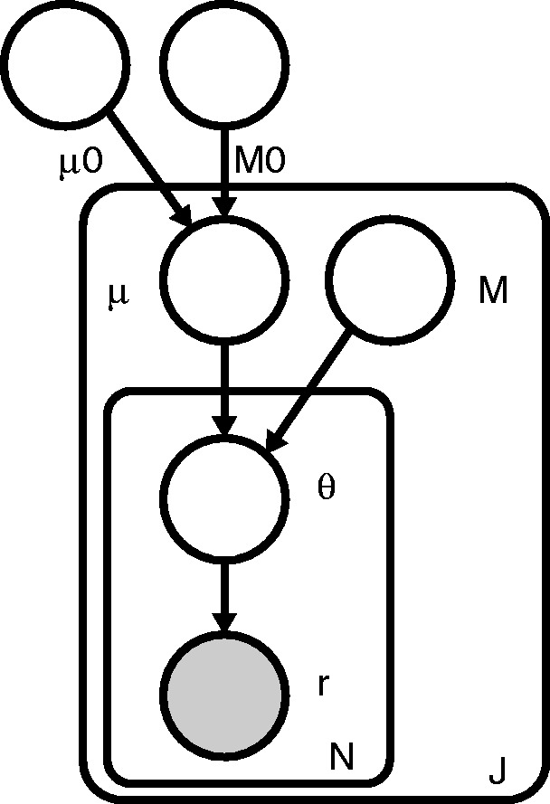
RVD2 graphical model

For a given sample, the observed data consist of two matrices $r\in R^{J\times N}$ and $n\in R^{J\times N}$, where r_ji is the number of reads with a non-reference base at location j in experimental replicate i and n_ji is the total number of reads at location j in replicate i. J is the region of interest length and N is the number of technical replicates in the sample. Technical replicates are used to establish experimental variability in NGS procedure (Robasky et al., 2013), though multiple replicates are not necessary for RVD2.

The model generative process given hyperparameters ${\mu }_0,M_0$ and M is as follows:

1. For each location j:

   1. Draw an error rate ${\mu }_j\sim \text{Beta}({\mu }_0,M_0)$
   2. For each replicate i:

      1. Draw ${\theta }_{ji}\sim \text{Beta}({\mu }_j,M_j)$
      2. Draw $r_{ji}|n_{ji}\sim \text{Binomial}({\theta }_{ji},n_{ji})$

The generative process involves several hyperparameters: μ₀, a global error rate; M₀, a global precision; μ_j, a local error rate; and M_j, a local precision. The global error rate, μ₀, estimates the expected error rate across all locations. The global precision, M₀, estimates the variation in the error rate across locations. The local error rate, μ_j, estimates the expected error rate across replicates at location j. The local precision, M_j, estimates the variation in the error rate across replicates at location j.

RVD2 has three levels of sampling. First, a global error rate and global precision are chosen once for the entire dataset. Then, at each location, a local precision is chosen and a local error rate is sampled from a Beta distribution. Finally, the error rate for replicate i at location j is drawn from a Beta distribution and the number of non-reference reads is drawn from a binomial.

RVD2 hierarchically partitions sources of variation in the data. The distribution $r_{ji}|n_{ji}\sim \text{Binomial}({\theta }_{ji},n_{ji})$ models the variation due to sampling the pool of DNA molecules on the sequencer. The distribution ${\theta }_{ji}\sim \text{Beta}({\mu }_j,M_j)$ models the variation due to experimental reproducibility. The variation in error rate due to sequence context is modeled by ${\mu }_j\sim \text{Beta}({\mu }_0,M_0)$. Importantly, increasing the read depth n_ji only reduces the sampling error, but does nothing to reduce experimental variation or variation due to sequence context.

The joint distribution over the latent and observed variables for data at location j in replicate i given the parameters can be factorized as

$$\begin{array}{c}p\left(r_{ji},{\theta }_{ji},{\mu }_j|n_{ji};{\mu }_0,M_0,M_j\right)=p\left(r_{ji}|{\theta }_{ji},n_{ji}\right)p\left({\theta }_{ji}|{\mu }_j;M_j\right)p\left({\mu }_j;{\mu }_0,M_0\right),\\ p\left(r_{ji}|{\theta }_{ji},n_{ji}\right)=\frac{\Gamma (n_{ji}+1)}{\Gamma (r_{ji}+1)\Gamma (n_{ji}-r_{ji}+1)}·{\theta }_{ji}^{r_{ji}}{(1-{\theta }_{ji})}^{n_{ji}-r_{ji}},\\ p\left({\theta }_{ji}|{\mu }_j;M_j\right)=\frac{{\theta }_{ji}^{M_j{\mu }_j-1}{(1-{\theta }_{ji})}^{M_j(1-{\mu }_j)-1}}{B(M_j{\mu }_j,M_j(1-{\mu }_j))},\\ p\left({\mu }_j;{\mu }_0,M_0\right)=\frac{{\mu }_j^{M_0{\mu }_0-1}{(1-{\mu }_j)}^{M_0(1-{\mu }_0)-1}}{B(M_0{\mu }_0,M_0(1-{\mu }_0))},\end{array}$$ (1)

where B$(·,·)$ denotes the beta function.

The log-likelihood of the dataset is

$$\begin{array}{l}\log p\left(r|n;{\mu }_0,M_0,M\right)={\displaystyle \sum _{j=1}^J{\displaystyle \sum _{i=1}^N\log }}{\displaystyle {\int }_{{\mu }_j}{\displaystyle {\int }_{{\theta }_{ji}}p}}\left(r_{ji}|{\theta }_{ji},n_{ji}\right)\\ p\left({\theta }_{ji}|{\mu }_j;M_j\right)p\left({\mu }_j;{\mu }_0,M_0\right)d{\theta }_{ji}d{\mu }_j.\end{array}$$ (2)

RVD2 improves on RVD in three ways. First, RVD2 has a $\text{Beta}({\mu }_0,M_0)$ prior on local error rate μ_j, which captures the global across-position error rate. The prior distribution allows μ_j to share information across adjacent positions and allows RVD2 to handle low read depths. Second, RVD2 handles multiple replicates in case samples. Third, RVD2 has a more accurate Bayesian hypothesis testing method compared with the normal z-test in RVD. We show a performance comparison between RVD and RVD2 in Section 5.2.

3 Inference and Hypothesis Testing

The primary object of inference in this model is the joint posterior distribution function over the latent variables,

$$p(\mu ,\theta |r,n;\varphi )=\frac{p(\mu ,\theta ,r|n;\varphi )}{p(r|n;\varphi )},$$ (3)

where the parameters are $\varphi {\displaystyle \stackrel{\Delta }{=}}\{{\mu }_0,M_0,M\}$.

The Beta distribution over μ_j is conjugate to the Binomial distribution over θ_ji, so we can write the posterior distribution as a Beta distribution. However, there is not a closed form for the product of a Beta distribution with another Beta distribution, so exact inference is intractable.

Instead, we have developed a Metropolis-within-Gibbs (MwG) approximate inference algorithm shown in Algorithm 1. First, the hyperparameters are initialized using method-of-moments (MoM). Given those hyperparameter estimates, we sample from the marginal posterior distribution for μ_j given its Markov blanket using a Metropolis–Hasting (M–H) rejection sampling rule. Finally, we sample from the marginal posterior distribution for θ_ji given its Markov blanket. Samples from θ_ji can be drawn from the posterior distribution directly because the prior and likelihood form a conjugate pair. This sampling procedure is repeated until the chain converges to a stationary distribution and then we draw samples from the posterior distribution over latent variables.

Algorithm 1 Metropolis-within-Gibbs Algorithm —

1: Initialize θ, μ, M, μ₀, M₀

2: repeat

3: for each location j do

4: Draw T samples from $p\left({\mu }_j|{\theta }_{ij},{\mu }_0,M_0\right)$ using M–H

5: Set μ_j to the sample median for the T samples

6:  for each replicate i do

7:   Sample from $p\left({\theta }_{ij}|r_{ij},n_{ij},{\mu }_j,M\right)$

8:  end for

9: end for

10: until sample size sufficient

3.1 Initialization

The initial values for the model parameters and latent variables are obtained by a MoM procedure. MoM works by setting the population moment equal to the sample moment. A system of equations is formed such that the number of moment equations is equal to the number of unknown parameters and the equations are solved simultaneously to give the parameter estimates. We simply start with the data matrices r and n and work up the hierarchy of the graphical model solving for the parameters of each conditional distribution in turn.

We present the initial parameter estimates here and provide the derivations in Supplementary Information. The MoM estimate for replicate-level parameters are ${\widehat{\theta }}_{ji}=\frac{r_{ji}}{n_{ji}}$. The estimates for the local parameters are ${\widehat{\mu }}_j=\frac{1}{N}{\sum }_{i=1}^N{\widehat{\theta }}_{ji}$ and $\widehat{{\widehat{M}}_j}=\frac{{\widehat{\mu }}_j(1-{\widehat{\mu }}_j)}{\frac{1}{N}{\sum }_{i=1}^N{\widehat{\theta }}_{ji}^2}-1$. The estimates for the global parameters are ${\widehat{\mu }}_0=\frac{1}{J}{\sum }_{j=1}^J{\widehat{\mu }}_j$ and ${\widehat{M}}_0=\frac{{\widehat{\mu }}_0(1-{\widehat{\mu }}_0)}{\frac{1}{J}{\sum }_{j=1}^J{\widehat{\mu }}_j^2}-1$.

3.2 Sampling from $p\left({\theta }_{ij}|r_{ij},n_{ij},{\mu }_j,M\right)$

Samples from the posterior distribution $p({\theta }_{ji}|r_{ji},n_{ji},{\mu }_j,M_j)$ are drawn analytically because of the Bayesian conjugacy between the prior $p({\theta }_{ji}|{\mu }_j,M_j)\sim \text{Beta}({\mu }_j,M_j)$ and the likelihood $p(r_{ji}|n_{ji},{\theta }_{ji})\sim \text{Binomial}({\theta }_{ji},n_{ji})$. The posterior distribution is

$$p({\theta }_{ji}|r_{ji},n_{ji},{\mu }_j,M_j)\sim \text{Beta}\left(r_{ji}+M_j{\mu }_j,n_{ji}-r_{ji}+M_j(1-{\mu }_j)\right).$$ (4)

3.3 Sampling from $p\left({\mu }_j|{\theta }_{ji},M_j,{\mu }_0,M_0\right)$

The posterior distribution over μ_j given its Markov blanket is

$$p({\mu }_j|{\theta }_{ji},M_j,{\mu }_0,M_0)\propto p({\mu }_j|{\mu }_0,M_0)p({\theta }_{ji}|{\mu }_j,M_j)$$ (5)

Since the prior, $p({\mu }_j|{\mu }_0,M_0)$, is not conjugate to the likelihood, $p({\theta }_{ji}|{\mu }_j,M_j)$, we cannot write an analytical form for the posterior distribution. Instead, we sample from the posterior distribution using the M–H algorithm.

A candidate sample is generated from the symmetric proposal distribution $Q\left({\mu }_j^{*}|{\mu }_j^{(p)}\right)\sim \mathcal{N}\left({\mu }_j^{(p)},{\sigma }_j^{(p)}\right)$, where ${\mu }_j^{(p)}$ is the pth from the posterior distribution. The acceptance probability is then

$$a=\frac{p({\mu }_j^{*}|{\mu }_0,M_0)p({\theta }_{ji}^{(p+1)}|{\mu }_j^{*},M_j)}{p({\mu }_j^{(p)}|{\mu }_0,M_0)p({\theta }_{ji}^{(p+1)}|{\mu }_j^{(p)},M_j)}.$$ (6)

We fixed the proposal distribution variance for all the M–H steps within a Gibbs iteration to ${\sigma }_j=0.1·{\widehat{\mu }}_j·(1-{\widehat{\mu }}_j)$ if ${\widehat{\mu }}_j\in ({10}^{-3},1-{10}^{-3})$ and ${\sigma }_j={10}^{-4}$ otherwise, where ${\widehat{\mu }}_j$ is the MoM estimator of μ_j. Though it is not theoretically necessary, we have found that the algorithm performance improves when we take the median of five or more M–H samples in single Gibbs step for each position.

We resample from the proposal if the sample is outside of the support of the posterior distribution. We typically discard 20% of the sample for burn-in and thin the chain by a factor of 2 to reduce autocorrelation among samples. Since, each position j is exchangeable given the global hyperparameters, μ₀ and M₀, this sampling step can be distributed across up to J processors.

3.4 Posterior distribution test

3.4.1 Posterior difference test

MwG provides samples from the posterior distribution of μ_j given the case or control data. For notational simplicity, we define the random variables associated with these two distributions ${\mu }_j^{\text{case}}$ and ${\mu }_j^{\text{control}}$ and the associated samples as ${\tilde{\mu }}_j^{\text{case}}$ and ${\tilde{\mu }}_j^{\text{control}}$.

A variant is called if ${\mu }_j^{\text{case}}>{\mu }_j^{\text{control}}$ with high confidence,

$$\mathrm{Pr}({\mu }_j^{\text{case}}-{\mu }_j^{\text{control}}>\tau )\approx \frac{1}{N_{\text{MwG}}}{\displaystyle \sum _{k=1}^{N_{\text{MwG}}} }{\mathbb{1}}_{{\tilde{\mu }}_{jk}^{\text{case}}-{\tilde{\mu }}_{jk}^{\text{control}}>\tau }>1-\alpha ,$$ (7)

where τ is a detection threshold and $1-\alpha$ is a confidence level. We draw a sample from the posterior distribution ${\tilde{\mu }}_j^{\Delta }{\displaystyle \stackrel{\Delta }{=}}{\tilde{\mu }}_j^{\text{case}}-{\tilde{\mu }}_j^{\text{control}}$ by simple random sampling with replacement from ${\tilde{\mu }}_j^{\text{case}}$ and ${\tilde{\mu }}_j^{\text{control}}$.

The threshold, τ, may be set to 0 or optimized for a given median depth and desired MAF detection limit. The optimal τ maximizes the Matthews Correlation Coefficient (MCC),

$${\tau }^{*}=\underset{\tau }{\arg \max }\left\{\text{MCC}(\tau )\right\}.$$ (8)

While we are able to compute the optimal τ threshold for a test dataset, in general we would not have access to ${\tau }^{*}$. With sufficient training data, one would be able to develop a lookup table or calibration curve to set τ based on read depth and MAF level of interest. Absent this information we set τ = 0.

3.4.2 Posterior somatic test

We use a two-sided posterior difference test with control and case paired samples to identify somatic mutations. We consider scenarios when the case(tumor) error rate is lower than the control(germline) error rate (e.g. loss-of-heterozygosity) as well as scenarios when the case(tumor) error rate is higher than the control(germline) error rate (e.g. homozygous somatic mutation). The two hypothesis tests are then $\mathrm{Pr}({\mu }_j^{\text{case}}-{\mu }_j^{\text{control}}>\tau )>1-\alpha$ and $\mathrm{Pr}({\mu }_j^{\text{case}}-{\mu }_j^{\text{control}}<-\tau )>1-\alpha$. We typically set the threshold τ to 0.

3.4.3 Posterior germline test

We use a one-sided posterior distribution test with a single control sample to identify germline mutations. We call a germline mutation if ${\mu }_j^{\text{control}}\ge \tau$ with high confidence,

$$\mathrm{Pr}({\mu }_j^{\text{control}}\ge \tau )\approx \frac{1}{N_{\text{MwG}}}{\displaystyle \sum _{k=1}^{N_{\text{MwG}}} }{\mathbb{1}}_{{\tilde{\mu }}_{jk}^{\text{control}}\ge \tau }>1-\alpha .$$ (9)

3.5 ${\chi }^2$ test for non-uniform base distribution

An abundance of non-reference bases at a position called by the posterior density test may be due to a true mutation or due to a random sequencing error; we would like to differentiate these two scenarios. We assume non-reference read counts caused by a non-biological mechanism results in a uniform distribution over three non-reference bases. In contrast, the distribution of counts among three non-reference bases caused by biological mutation would not be uniform.

We use a ${\chi }^2$ goodness-of-fit test on a multinomial distribution over the non-reference bases to distinguish these two possible scenarios. The null hypothesis is $H_0:p=(p_1,p_2,p_3)$ where $p_1=p_2=p_3=1/3$. Cressie and Read (1984) identified a power-divergence family of statistics, indexed by λ, that includes as special cases Pearson’s ${\chi }^2(\lambda =1)$ statistic, the log likelihood ratio statistic $(\lambda =0)$, the Freeman–Tukey statistic $(\lambda =-1/2)$, and the Neyman modified statistic $X^2(\lambda =-2)$. The test statistic is

$$2n{I}^{\lambda }=\frac{2}{\lambda (\lambda +1)}{\displaystyle \sum _{k=1}^3{r}_{ji}^{(k)}}\left[{\left(\frac{r_{ji}^{(k)}}{E_{ji}^{(k)}}\right)}^{\lambda }-1\right];\lambda \in R,$$ (10)

where $r_{ji}^{(k)}$ is the observed frequency for non-reference base k at position j in replicate i and $E_{ji}^{(k)}$ is the corresponding expected frequency under the null hypothesis. Cressie and Read (1984) recommended $\lambda =2/3$ when no knowledge of the alternative distribution is available and we choose that value.

We control for multiple hypothesis testing in two ways. We use Fisher’s combined probability test (Fisher et al., 1970) to combine the P-values for N replicates into a single P-value at position j,

$${\chi }_j^2=-2{\displaystyle \sum _{i=1}^N\ln }(p_{ji}).$$ (11)

Equation (11) gives a test statistic that follows a ${\chi }^2$ distribution with 2N degrees of freedom when the null hypothesis is true. If the sample average depth is higher than 500, we use the Benjamini–Hochberg method to control the family-wise error rate over positions that have been called by the posterior distribution test (Benjamini and Hochberg, 1995; Efron, 2010). The average depth threshold is set because Benjamini–Hochberg method is a highly conservative method and will reject many true calls when the read depth is not high enough.

4 Datasets

We used two independent datasets to evaluate the performance of RVD2 and compare it with other variant calling algorithms. The synthetic DNA sequence data provide true positive and true negative positions as well as define minor allele fractions. The HCC1187 data is used to test the performance on a sequenced cancer genome with less than 100% tumor purity.

4.1 Synthetic DNA sequence data

4.1.1 Experimental methods

Two 400 bp DNA sequences (including linkers) that are identical except at 14 loci with variant bases were synthesized and clonally isolated. The samples with the mutations are taken as the case sample and the sample without the mutations is taken as the control. Aliquots of the case and control DNA were mixed at defined fractions to yield defined minor allele fractions (MAFs) of 0.1, 0.3, 1, 10 and 100%. Paired-end sequencing was performed on an Illumina GAIIx sequencer (Illumina SCS 2.8) with real-time image analysis and base calling (Illumina RTA 2.8). Eland II (from Illumina pipeline version 1.6) was used with the default parameters to perform sequence alignment to the 300-bp synthetic DNA construct. More details of the experimental protocol are available from the original publication (Flaherty et al., 2011). As shown in Supplementary Table S1, each sample has ∼1 000 000 35 bp paired end reads.

4.1.2 Pre-processing methods

The reads were aligned with Eland as described previously. We then ran samtools mpileup with the -C50 option to filter for high mapping quality reads. To simulate lower coverage data while retaining the error structure of real NGS data, BAM files for the synthetic DNA data were downsampled $10\times , 100\times , 1000\times$ and $10\hspace{0.17em}000\times$ using Picard v1.96. The final dataset contains read pairs for three replicates of each case and pairs of reads three replicates for the control sample giving N = 6 replicates for the control and each MAF level.

4.2 HCC1187 sequence data

4.2.1 Experimental methods

The HCC1187 dataset is a well-recognized baseline dataset from Illumina for evaluating sequence analysis algorithms (Howarth et al., 2011, 2007; Newman et al., 2013). The HCC1187 cell line was derived from epithelial cells from primary breast tissue from a 41–year-old adult with TNM stage IIA primary ductal carcinoma. The estimated tumor purity was reported to be 0.8. Matched normal cells were derived from lymphoblastoid cells from peripheral blood. Sequencing libraries were prepared according to the protocol described in the original technical report (Allen, 2013).

4.2.2 Pre-processing methods

The raw FASTQ read files were aligned to hg19 using the Isaac aligner to generate BAM files (Raczy et al., 2013). The aligned data had an average read depth of 40× for the normal sample and 90× for the tumor sample with about 96% coverage with 10 or more reads. We used samtools mpileup to generate pileup files using hg19 as reference sequence (Navin et al., 2010).

5 Results

We tested RVD2 using synthetic DNA and data from the HCC1187 primary ductal carcinoma sample. The inference algorithm parameters were set to yield 4000 Gibbs samples with a 20% burn-in and $2\times$ thinning rate for a final total of 1600 samples. We drew 1000 samples from ${\tilde{\mu }}^{\Delta }={\tilde{\mu }}_j^{\text{case}}-{\tilde{\mu }}_j^{\text{control}}$ to estimate the posterior probability of a variant.

We performed the posterior difference test to identify mutations in the haploid synthetic data. We set the threshold τ = 0 and the size of the test $\alpha =0.05$.

For the HCC1187 dataset, we identified both somatic and germline mutations. In the posterior somatic test, we set the threshold τ = 0 and the size of the test $\alpha =0.05$. In the posterior germline test, we set the threshold $\tau =0.05$ considering the low average coverage (40×). The size of the test is set at $\alpha =0.15$. We performed the ${\chi }^2$ non-uniformity test after the posterior density tests.

5.1 Performance by read depth

We generated receiver-operating characteristic curves (ROCs) for a range of median read depth and a range of MAFs. For these ROCs, we used the posterior density test without the ${\chi }^2$ test to evaluate the performance of posterior density test individually. Figure 2 shows ROCs generated by varying the threshold τ with a fixed $\alpha =0.05$. Figure 2a shows ROC curves for a true 0.1% MAF for a range of median coverage depths. At the lowest depth the sensitivity and specificity is no better than random. However, we would not expect to be able to call a 1 in 1000 variant base with a coverage of only 43. The performance improves monotonically with read depth. Figure 2b and c shows a similar relationship between coverage depth and accuracy for higher MAFs.

Fig. 2.

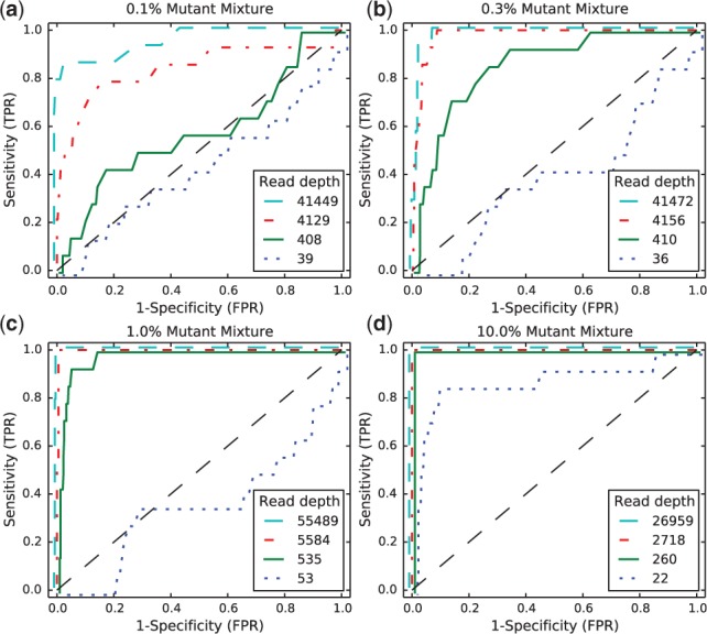
ROCs varying read depth showing detection performance

We measured the computational time for RVD2 varying the number of Gibbs sampling steps and the median read depth for the 400 bp synthetic dataset. In brief, on a 2.4-GHz processor it took ∼13 min per 1000 Gibbs samples to fit the model. The computational time is independent of the median read depth due to the model structure; the same performance was observed for a median read depth of 130 and 40 000. As stated previously, due to the independence structure of the model, we are able to perform the sampling step for each location in parallel greatly decreasing the computational time. The memory requirement is roughly the size of the gene sequence times the number of Gibbs samples. Complete timing results without parallelization are shown in Supplementary Section 8.

5.2 Empirical performance compared with other algorithms

We compare the empirical performance of RVD2 to other variant calling algorithms using the synthetic DNA dataset by the false discovery rate (FDR) and sensitivity/specificity. Among these algorithms, Samtools and GATK are optimized for homogeneous samples, while RVD, VarScan2-somatic, Strelka and muTect have good performance to call variants in heterogeneous samples. In research applications, the FDR is a more relevant performance metric because the aim is generally to identify interesting variants for follow-up. The sensitivity/specificity metric is more relevant in clinical applications where one is more interested in correctly calling all of the positive variants and none of the negatives. GATK, Varscan2, Strelka and muTect are only able to make use of one case and one control sample, so we provide results of RVD2 with the same data set (N = 1) for comparison.

We compare the empirical performance across a wide range of median read depth (∼40× to ∼40 000×). In typical whole genome applications, the read depth is between 10× and 100×. For targeted cancer sequencing, the median read depth is higher at 100× to 1000×. For microbial or viral sequencing for rare variants, the median read depth is even higher at 1000× to 100  000×.

5.2.1 Sensitivity/specificity comparison

Figure 3 shows that samtools, GATK and VarScan2-mpileup all have similar performance. They call the 100% MAF experiment well even at low depth, but are unable to identify true variants in mixed samples. VarScan2-somatic is able to call more mixed samples. However, as the read depth increases the specificity degrades. Strelka is able to call 10% MAF variants with good performance, but is limited at 1% MAF and below. muTect has good performance across a wide range of MAF levels. But even at the highest depth only has around 0.5 sensitivity for low MAF levels.

Fig. 3.

Sensitivity/specificity comparison of RVD2 with other variant calling algorithms using synthetic DNA data

The performance statistics for RVD are an average of three sets of pair-end case replicates. RVD performed the best among all algorithms when the read depth is near 40 000. RVD called all the mutated positions across all MAF levels with no false positives when MAF level is 0.3% or lower. However, RVD cannot call any mutations when the depth is too low to measure the baseline error rate and therefore is not useful for low-depth data.

RVD2 has a high sensitivity and specificity for a broad range of read depths and MAFs. The sensitivity increases considerably with read depth at a slight expense to specificity. For the most difficult test with a low read depth and low MAF, RVD2 performs on-par with muTect. With ${\tau }^{*}$ the performance is much better with high sensitivity and specificity across a wide range of read depths and MAFs. However, in practice one may not know the optimal ${\tau }^{*}$ a priori. With N = 6 replicates, the sensitivity increases considerably for low MAF variants with a slight degradation in specificity due to false positives. When the median read depth is at least $10\times$ the MAF, RVD2 has higher specificity than all of the other algorithms tested and has a lower sensitivity in only three cases.

5.2.2 FDR comparison

Figure 4 shows the FDR for RVD2 compared with samtools, GATK, varscan, Strelka and muTect. Blank cells indicate no positive calls were made.

Fig. 4.

FDR comparison of RVD2 with other variant calling algorithms using synthetic DNA data. Blank cells indicate no locations were called variant

Samtools performs well on 100% MAF sample and performance improves for read depths 3089 and 30 590. GATK performs well on both the 10 and 100% variants, but makes a false positive call at the 100% MAF level for all read depth levels. VarScan2-pileup performs perfectly for all but the lowest depth for the 100% MAF.

VarScan2-somatic is able to make calls for all but the lowest MAF and coverage level. However, the FDR is high due to many false positives. Interestingly, at a MAF of 100% the FDR is zero for lowest read depth and over 0.9 for the highest read depth. Strelka has a better FDR than the samtools, GATK or Varscan2-somatic algorithms for almost all read depths at the 10 and 100% MAF. However, it does not call any variants at or below 1% MAF. muTect has the best FDR performance of the other algorithms we tested over a wide range of MAF and depths. But the FDR level is relatively high at around 0.7 for 0.1–1% MAF and 0.3 for 10–100% MAF. RVD has best FDR performance in the high read depth for 0.1–1% MAF levels. The FDR increases to around 0.3 for 10–100% MAF in the high read depth.

RVD2 has a lower FDR than other algorithms when the read depth is greater than $10\times$ the inverse MAF with N = 1 and τ set to the default value of zero or to the optimal value. The FDR is higher when N = 6 because the variance of the control error rate distribution $P({\mu }_j^{\text{control}}|r^{\text{control}})$ is smaller. The smaller variance yields improvements in sensitivity at the expense of more false positives. Since the FDR only considers positive calls, the performance by that measure degrades.

5.3 HCC1187 primary ductal carcinoma sample

RVD2 identified 15 variant locations in the 59 kbp PAXIP1 gene from chr7:154735400 to chr7:154794682. There were 11 germline variants and 10 somatic mutations. Figure 5 shows the estimated MAFs for the normal and tumor samples at the called locations. Interestingly, positions chr7:154754371 and chr7:154758813 appear to be loss-of-heterozygosity events. Some of these mutations are also found to be common population SNPs according to dbSNPv138. The corresponding identities are shown in Figure 5. The read depth distribution for positions called by RVD2 is provided in Supplementary Table S1. Karyotyping indicates that chromosome 7 in HCC1187 is tetraploid http://www.path.cam.ac.uk/pawefish/BreastCellLineDescriptions/HCC1187.html.

Fig. 5.

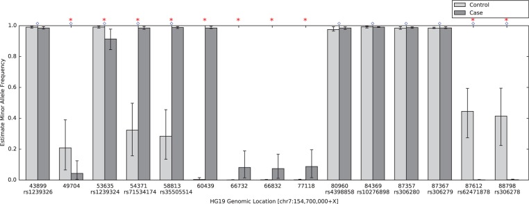
Estimated minor allele fraction for germline and somatic mutations called by RVD2 in the 59kbp PAXIP1 gene. Blue diamonds indicate germline mutations, where ${\mu }^{\text{control}}$ is significantly different from the reference sequence. Red stars indicate somatic mutations, where ${\mu }^{\text{case}}$ is significantly different from ${\mu }^{\text{control}}$. The vertical lines represent 95% credible interval around posterior mean MAF. Ten positions are common population SNPs according to dbSNPv138, and the identities are shown below the positions

5.3.1 Performance comparison with other algorithms

We ran muTect and VarScan2-somatic to call mutations in the PAXIP1 gene in HCC1187 sample. We also compared with the result shown in original research report where Strelka was used to identify mutations in the same sample (Allen, 2013). Figure 6a shows mutation detection result from Strelka, RVD2, muTect and VarScan2-somatic. For notation simplicity, we use position index to present actual positions in Figure 6 (the corresponding genomic positions are provided in Supplementary Table S1).

Fig. 6.

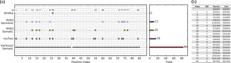
(a) Positions called by VarScan2-somatic, muTect, RVD2 and Strelka in the 59kbp PAXIP1 gene from chr7:154735400 to chr7:154794682. The positions are sorted by index (correspondence to genomic positions shown in Supplementary Table S1). (b) Read counts for each base for positions called by RVD2 and muTect from raw pileup data

The mutations called by RVD2 and muTect are the most consistent among all the techniques. RVD2 detected 15 germline mutations and 10 somatic mutations, while muTect reported 16 mutations; 11 were called by both. In the disagreements, RVD2 did not call positions 1, 39, 54 and 84 while muTect did not call positions 41 75 and 77. Referring to the depth distribution shown in Figure 6b, it can be seen that positions 41, 75 and 77 are more likely mutated while positions 1, 39, 54 and 84 are less likely mutated.

Strelka was the least sensitive algorithm among all the algorithms. According to the technical report, Strelka identified position 26 (chr7:154760439) as variant, but did not call any other variants. In particular Strelka missed the two LOH events called by RVD2. VarScan2-somatic called most positions among all algorithms, 84 positions as shown in Figure 6a. VarScan2-somatic detected all the positions called by RVD2 except position 39, which turns out to be a very likely mutation given the depth distribution in Figure 6b. VarScan2-somatic reported 65 positions which were not called by any other three algorithms. The read depth in Supplementary Table S1 suggests that these positions are very likely to be false positives. As shown in Figure 4, the FDR for VarScan2-somatic at read depth 53 MAF level 1.0% is as high as 1.00. Spencer et al. (2013) also mentioned that VarScan2 has tendency to call many false positives at high read depth.

6 Discussion

We describe here a novel algorithm for model estimation and hypothesis testing for identifying single-nucleotide variants in heterogeneous samples using NGS data. Our algorithm has a higher sensitivity and specificity than many other approaches for a range of read depths and MAFs.

Our inference algorithm uses Gibbs sampling to do inference in the RVD2 hierarchical empirical Bayes model. This sampling procedure provides a guarantee to identify the global optimal parameter settings asymptotically. However, it may require many samples to achieve that guarantee causing the algorithm to be slower than other deterministic approaches. We opted for this balance of speed and accuracy because computational time is often not limiting and the cost of a false positive or false negative greatly outweighs the cost of more computation. Another factor that can affect the speed of RVD2 is the number of M–H sample within one Gibbs sampling run. RVD2 is able to use multiple cores in parallel, which can significantly improve time efficiency. In future studies, we plan to reduce the computational cost by using more sophisticated MCMC sampling methods or deterministic approximation methods such as variational EM or stochastic variational EM.

We have focused on the statistical model and hypothesis test in this study and our results do not include any pre-filtration of erroneous reads or post-filtration of mutation calls beyond a simple quality score threshold. Incorporation of such data-cleaning steps will likely improve the accuracy of the algorithm.

Our approach does not address identification of indels, structural variants or copy number variants. Those mutations typically require specific data analysis models and tests that are different than those for single-nucleotide variants. Furthermore, analysis of RNA-seq data or other data generated on the NGS platform may require different models that are more appropriately tuned to the particular noise feature of that data.

The availability of clinical sequence data is increasing as the technical capability to sequence clinical samples at low-cost improves. Consequently, we require statistically accurate algorithms that are able to call germline and somatic point mutations in heterogeneous samples with low purity. Such accurate algorithms are a step toward greater access to genomics for clinical diagnostics.

References

- 1000 Genomes Project Consortium et al. (2012) An integrated map of genetic variation from 1,092 human genomes. Nature, 491, 56–65. [DOI] [PMC free article] [PubMed] [Google Scholar]
- Alkan C., et al. (2009) Personalized copy number and segmental duplication maps using next-generation sequencing. Nat. Genet., 41, 1061–1067. [DOI] [PMC free article] [PubMed] [Google Scholar]
- Allen E. (2013) Molecular characterization of tumors using next-generation sequencing. Technical Report 770‐2013‐011, 2013 Illumina, Inc. [Google Scholar]
- Benjamini Y., Hochberg Y. (1995) Controlling the false discovery rate: a practical and powerful approach to multiple testing. J. R. Stat. Soc. B 57, 289–300. [Google Scholar]
- Capobianchi M.R., et al. (2012) Next-generation sequencing technology in clinical virology. Clin. Microbiol. Infect., 19, 15–22. [DOI] [PubMed] [Google Scholar]
- Cibulskis K., et al. (2013) Sensitive detection of somatic point mutations in impure and heterogeneous cancer samples. Nature, 31, 213–219. [DOI] [PMC free article] [PubMed] [Google Scholar]
- Cressie N., Read T.R. (1984) Multinomial goodness-of-fit tests. J. R. Stat. Soc. B, 46, 440–464. [Google Scholar]
- Cushing A., et al. (2013) Rvd: a command-line program for ultrasensitive rare single nucleotide variant detection using targeted next-generation DNA resequencing. BMC Res. Notes, 6, 206. [DOI] [PMC free article] [PubMed] [Google Scholar]
- DePristo M.A., et al. (2011) A framework for variation discovery and genotyping using next-generation DNA sequencing data. Nat. Genet., 43, 491–498. [DOI] [PMC free article] [PubMed] [Google Scholar]
- Efron B. (2010) Large-Scale Inference: Empirical Bayes Methods for Estimation, Testing, and Prediction, vol. 1 Cambridge University Press, Cambridge, MA. [Google Scholar]
- Fan H.C., et al. (2008) Noninvasive diagnosis of fetal aneuploidy by shotgun sequencing DNA from maternal blood. PNAS, 105, 16266–16271. [DOI] [PMC free article] [PubMed] [Google Scholar]
- Fisher S.R.A., et al. (1970) Statistical Methods for Research Workers, vol. 14 Oliver and Boyd Edinburgh, Provo, UT. [Google Scholar]
- Flaherty P., et al. (2011) Ultrasensitive detection of rare mutations using next-generation targeted resequencing. Nucleic Acids Res., 40, e2. [DOI] [PMC free article] [PubMed] [Google Scholar]
- Ghedin E., et al. (2010) Deep sequencing reveals mixed infection with 2009 pandemic influenza A (H1N1) virus strains and the emergence of oseltamivir resistance. J. Infect. Dis., 203, 168–174. [DOI] [PMC free article] [PubMed] [Google Scholar]
- Howarth K., et al. (2007) Array painting reveals a high frequency of balanced translocations in breast cancer cell lines that break in cancer-relevant genes. Oncogene, 27, 3345–3359. [DOI] [PMC free article] [PubMed] [Google Scholar]
- Howarth K.D., et al. (2011) Large duplications at reciprocal translocation breakpoints that might be the counterpart of large deletions and could arise from stalled replication bubbles. Genome Res., 21, 525–534. [DOI] [PMC free article] [PubMed] [Google Scholar]
- Jordan M.I. (2004). Graphical models. Stat. Sci., 19, 140–155. [Google Scholar]
- Kitzman J.O., et al. (2012) Noninvasive whole-genome sequencing of a human fetus. Sci. Transl. Med., 4, 137ra76–137ra76. [DOI] [PMC free article] [PubMed] [Google Scholar]
- Koboldt D.C., et al. (2012) VarScan 2: somatic mutation and copy number alteration discovery in cancer by exome sequencing. Genome Res., 22, 568–576. [DOI] [PMC free article] [PubMed] [Google Scholar]
- Koboldt D.C., et al. (2013) The next-generation sequencing revolution and its impact on genomics. Cell, 155, 27–38. [DOI] [PMC free article] [PubMed] [Google Scholar]
- Laird P.W. (2010) Principles and challenges of genomewide DNA methylation analysis. Nat. Rev. Genet., 11, 191–203. [DOI] [PubMed] [Google Scholar]
- Li H. (2011) A statistical framework for SNP calling, mutation discovery, association mapping and population genetical parameter estimation from sequencing data. Bioinformatics, 27, 2987–2993. [DOI] [PMC free article] [PubMed] [Google Scholar]
- McKenna A., et al. (2010) The genome analysis toolkit: a MapReduce framework for analyzing next-generation DNA sequencing data. Genome Res., 20, 1297–1303. [DOI] [PMC free article] [PubMed] [Google Scholar]
- Navin N., et al. (2010) Inferring tumor progression from genomic heterogeneity. Genome Res., 20, 68–80. [DOI] [PMC free article] [PubMed] [Google Scholar]
- Newman S., et al. (2013) The relative timing of mutations in a breast cancer genome. PLoS One, 8, e64991. [DOI] [PMC free article] [PubMed] [Google Scholar]
- Ouyang Z., et al. (2009) ChIP-Seq of transcription factors predicts absolute and differential gene expression in embryonic stem cells. PNAS, 106, 21521–21526. [DOI] [PMC free article] [PubMed] [Google Scholar]
- Quail M.A., et al. (2012) A tale of three next generation sequencingplatforms: comparison of Ion Torrent, PacificBiosciences and Illumina MiSeq sequencers. BMC Genomics, 13, 1–1. [DOI] [PMC free article] [PubMed] [Google Scholar]
- Raczy C., et al. (2013) Isaac: ultra-fast whole genome secondary analysis on illumina sequencing platforms. Bioinformatics, 29, 2041–2043. [DOI] [PubMed] [Google Scholar]
- Rivera C.M., Ren B. (2013) Mapping human epigenomes. Cell, 155, 39–55. [DOI] [PMC free article] [PubMed] [Google Scholar]
- Robasky K., et al. (2013) The role of replicates for error mitigation in next-generation sequencing. Nat. Rev. Genet., 15, 56–62. [DOI] [PMC free article] [PubMed] [Google Scholar]
- Saunders C.T., et al. (2012) Strelka: accurate somatic small-variant calling from sequenced tumor-normal sample pairs. Bioinformatics, 28, 1811–1817. [DOI] [PubMed] [Google Scholar]
- Spencer D.H., et al. (2013) Performance of common analysis methods for detecting low-frequency single nucleotide variants in targeted next-generation sequence data. J. Mol. Diagn., 16, 75–88. [DOI] [PMC free article] [PubMed] [Google Scholar]
- Stead L.F., et al. (2013) Accurately identifying low-allelic fraction variants in single samples with next-generation sequencing: applications in tumor subclone resolution. Hum. Mutat., 34, 1432–1438. [DOI] [PubMed] [Google Scholar]
- The Human Microbiome Project Consortium (2013) A framework for human microbiome research. Nature, 486, 215–221. [DOI] [PMC free article] [PubMed] [Google Scholar]
- Yau C., et al. (2010) A statistical approach for detecting genomic aberrations in heterogeneous tumor samples from single nucleotide polymorphism genotyping data. Genome Biol., 11, R92–R92. [DOI] [PMC free article] [PubMed] [Google Scholar]
- Zagordi O., et al. (2010) Error correction of next-generation sequencing data and reliable estimation of HIV quasispecies. Nucleic Acids Res., 38, 7400–7409. [DOI] [PMC free article] [PubMed] [Google Scholar]
Associated Data
This section collects any data citations, data availability statements, or supplementary materials included in this article.