Abstract
Neural networks offer a powerful new approach to information processing through their ability to generalize from a specific training data set. The success of this approach has raised interesting new possibilities of incorporating statistical methodology in order to enhance their predictive ability. This paper reports on two complementary methods of prediction. one using neural networks and the other using traditional statistical methods. The two methods are compared on the basis of their prediction applied to standardized developmental infant outcome measures using preselected infant and maternal variables measured at birth. Three neural network algorithms were employed. In our study, no one network outperformed the other two consistently. The neural networks provided significantly better results than the regression model in terms of variation and prediction of extreme outcomes. Finally we demonstrated that selection of relevant input variables through statistical means can produce a reduced network structure with no loss in predictive ability.
Keywords: feed forward MLP, functional link net (FLN), flat net, regression
1. Introduction
Neural network computation [14] continues to gain popularity as an information processing tool and has been applied to several problems in medical decision-making that traditionally have been attacked using statistical methods [1,4,10,11,14,23-26]. When neural network methodology is compared to statistical approaches to solve these problems, it is seen to have both advantages and disadvantages. On the positive side, neural networks are “model free” in that no a priori mathematical model must be assumed. Thus, expert knowledge about the process being modeled is not needed. Neural networks are also self-training and amenable to incremental training after being put into use. On the negative side, neural networks operate as “black boxes” in that they fail to elucidate any “deep” knowledge about the process being modeled. Further, since neural networks learn by example, training data must be available for use by the learning process.
We report on our experience in combining both statistical and neural network techniques in constructing predictive models in the context of a pediatric psychological study. In particular, we compare the predictive modeling capabilities of a linear regression model, three different neural network models, and a neural network model with statistical enhancement. The objective of this study was to identify ways in which statistical techniques can be incorporated into neural processing, thereby taking advantage of the strengths of each.
1.1. Neural Network Architectures
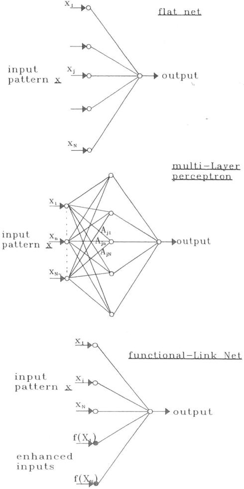
Among the many different neural network architectures that have been proposed, the most commonly used neural network structure for supervised learning is the multi-layer perceptron (MLP) [8,14]. An MLP is a network of simple processing nodes (“neurons”) arranged into an input layer, zero or more hidden layers, and an output layer. The layers are fully interconnected in that the output from each node of one layer is linked to the inputs of all of the nodes of the next layer. A second commonly-used neural network architecture is the flat net [14]. The flat net is a simplified version of the MLP in which there is no hidden layer. A third neural network architecture in use is the functional-link net (FLN) [14-16]. The FLN is a recent modification of the flat net in which functional enhancements of the original inputs are used as additional inputs to the network. These functional enhancements typically take the form of sinusoidal functions, power series, or random vectors. The enhancements provide the nonlinear dynamics that the additional layers in an MLP provide, but at a significantly lower algorithmic overhead. The three types of net work models are shown in Figure [1].
Figure I.
Three types of Neural Network Models: flat net, feed forward MLP and functional-link net.
1.2. Statistical Techniques
Several regression methodologies are available for statistical predictive modeling. Multiple logistic regression [9], discriminant analysis [13] and classification and regression trees [2] have been used for binary outcomes. For continuous outcomes, multiple linear regression, nonparametric regression, and generalized additive models [7] have been employed. The choice of any of these models is dependent on the dimensionality of the input variables. In low dimensional settings, piecewise polynomial fitting procedures based on splines [22] and locally weighted straight-line smoothers [3] are very popular non-parametric procedures. However, due to problems with surface smoothers in higher dimensional settings, several multivariate nonparametric regression techniques have been devised. Both recursive-partitioning regression [5] and projection-pursuit regression [12] methodologies attempt to approximate general functions in higher dimensions by adaptive computation. Friedman [6] presented the multivariate adaptive regression splines as a tool for flexible modeling of high dimensional data. Statistical pattern recognition based on Bayes’ decision rules has also been used. Here, classification techniques like discriminant analysis and nearest-neighbor methods are employed [17].
1.3. Objectives
Our overall goal in this work as well as in previous efforts and in ongoing parallel efforts is to construct a high quality predictive model in the context of an ongoing study of the medical, social, and developmental correlates of chronic lung disease during the ftrst three years of life [18-21]. Specifically, we want to predict developmental outcome at twelve months of age from data gathered at and immediately following birth. In this particular investigation, our goal was to determine the comparative advantages and disadvantages of several predictive models in this context, including models that combine statistical and neural network methodologies.
2. Methods
2.1. Data Collection
Data were obtained from an ongoing five-year prospective investigation of the medical, social, and developmental correlates of chronic lung disease during the first three years of life [18-21]. Twenty-eight variables capturing demographic factors and neonatal medical history believed to affect infant development during early childhood and two variables measuring developmental outcome at twelve months of age were selected for 331 study subjects. The outcome variables, chosen to be measurements of infant development, were the 12-month Bayley Mental Development Index (MDI) and the 12-month Bayley Psychomotor Development Index. (POI). The twenty-eight input variables are listed in Table [1].
Table 1.
Study Variables (N=272 to 331)
| Variable Name | N | Mean(SD) | Note |
|---|---|---|---|
| Bayley (Outcome Variables) | |||
| Mental Development Index 12 month (MDI) | 272 | 104(23) | continuous |
| Psychomotor Development 12 month (PDI) | 272 | 96(21) | continuous |
| Medical Risk (Input Variables) | |||
| Total Days on Supplemental Oxygen * | 303 | 29.2(44.1) | continuous |
| Intra-Ventricular Hemorrhaging (IVH) | 303 | 0.44(0.94) | continuous |
| Intra-Ventricular hemorrhaging (IVH) * | 303 | 0.23(0.42) | 0/1 |
| Neurological Malformation (NEURAL) | 303 | 0.003(0.057) | 0/1 |
| Seizures | 303 | 0.023(0.150) | 0/1 |
| Echodense Lesion | 303 | 0.116(0.320) | 0/1 |
| Cystic Periventricular Leukomalacia | 303 | 0.050(0.217) | 0/1 |
| Porencephaly on follow-up Sonogram | 303 | 0.026(0.161) | 0/1 |
| Post-Hemorrhaging | 303 | 0.056(0.231) | 0/1 |
| Ventriculo Peritoneal Shunt | 303 | 0.017(0.128) | 0/1 |
| Meninges (MENING) | 303 | 0.007(0.081) | 0/1 |
| Sum of IVH to MENING (MED_ACUM) | 303 | 0.528(1.088) | continuous |
| Sum of NEURAL to MENING (MED_ACUM2) * | 303 | 0.297(0.816) | continuous |
| MED_ACUM >0 | 303 | 0.281(0.450) | 0/1 |
| MED_ACUM2 >0 | 303 | 0.182(0.386) | 0/1 |
| Social/Demographic (Input Variables) | |||
| Maternal Cocaine Use * | 331 | 0.13(0.34) | 0/1 |
| Multiple Birth * | 331 | 0.24(0.43) | 0/1 |
| Bronchopulmonary Dysplasia * | 331 | 0.38(0.49) | 0/1 |
| Very Low Birthweight without BPD * | 331 | 0.24(0.43) | 0/1 |
| Very Low Birthweight with or without BPD | 331 | 0.62(0.49) | 0/1 |
| Healthy Term Control | 331 | 0.38(0.49) | 0/1 |
| Gestational Age in weeks * | 331 | 32.7(5.9) | continuous |
| Social Economic Status * | 321 | 3.67(1.06) | continuous |
| White Race * | 331 | 0.46(0.5) | 0/1 |
| Birthweight * | 330 | 1950(1192) | continuous |
| Primary Caregiver is Biological Mother * | 297 | 0.96(0.19) | 0/1 |
| Mother's Age at Birth * | 318 | 27.7(5.8) | continuous |
| Mother's Education * | 318 | 13.2(2.3) | continuous |
0/1: 0=NO, l=YES
= regression variables
Only subjects with complete data for all of the 30 selected variables were included in the final data set. This data set was randomly divided three times into a 200-record set for training and a 131 -record set for evaluation. This allowed for the performance of three independent trials for the fit of each predictive model that we investigated. The same data sets were used for construction of both statistical and neural network models. The neural network programmer and biostatistician were blinded to each other's efforts at this point in our work.
2.2. Baseline Statistical Model
For the statistical regression models, we used fourteen explanatory variables believed to play a role in early infant development to help predict the developmental outcome variables. Several approaches to construction of a statistical model for this data were investigated, including non-linear regression and logistic regression. We settled on a multiple regression model and did not pursue other candidate models further. The fourteen variables this linear regression model are those listed in Table [2].
Table 2.
Stepwise Regression; Predictive Model Variables
| Variable Name | MDI (set1) | MDI (set2) | MDI (set3) | PDI (set 1) | PDI (set 2) | PDI (set 3) |
|---|---|---|---|---|---|---|
| Total Days on Supplemental Oxygen | x | x | x | x | x | x |
| Intra-Ventricular hemorrhaging | x | x | x | |||
| Sum of NEURAL to MENING | x | x | x | x | x | x |
| Maternal Cocaine | x | x | x | |||
| Multiple Birth | x | x | x | x | x | x |
| Bronchopulmonary Dysplasia | x | x | x | |||
| Very Low Birthweight without BPD | x | x | ||||
| Gestational Age in weeks | x | |||||
| Social Economic Status | x | x | x | x | ||
| Race | x | x | x | |||
| Birthweight | x | |||||
| Primary Caregiver is Biological Mother | x | x | x | x | ||
| Mother's Age at Birth | x | |||||
| Mother's Education | x | x | x | x | x | |
| Coefficient of Determination (R2) | 0.34 | 0.34 | 0.33 | 0.36 | 0.38 | 0.36 |
| Total Degrees of Freedom (DF) | 138 | 132 | 139 | 139 | 133 | 139 |
x = Stepwise Regression Selected Variables
2.3. Baseline Neural Network Models
For each of the three neural network architectures under consideration, a network was trained using the 28 input variables and two output variables. In the case of the MLP, a hidden layer of fifteen nodes was used. In the case of the FLN, fifteen enhanced features of random vector type were used to supplement the 28 original features. In all cases, each neuron's activation function was sigmoidal with the momentum set to 0.001 and the learning parameter set to 0.005. Each network was trained for 200 iterations. We used neural network simulation software developed in-house by one of the authors (S.M. Hosseini-Nezhad).
2.4. Neural Network Models with Statistical Preprocessing
Beginning with the fourteen variables used in the linear regression described earlier, a stepwise linear regression was fit to the data. A variable was considered significant for entry into the stepwise model if the p-value associated with that variable was less than 0.4, and it was allowed to leave the model if the p-value was over 0.4.
The variables identified in the stepwise models were deemed to be more relevant to prediction of the outcomes than the variables omitted from the models. We used this reduced subset of “relevant” variables in the training of new neural network models of the same three architectures as described earlier. Once again, each network was trained for 200 iterations.
2.5. Comparison of Models
In all, we constructed seven predictive models: three baseline neural network models, one baseline regression model, and three statistically enhanced neural network models. We compared these models on the bases of both goodness of fit to training data and the ability to predict outcomes from previously unseen input data.
3. Results
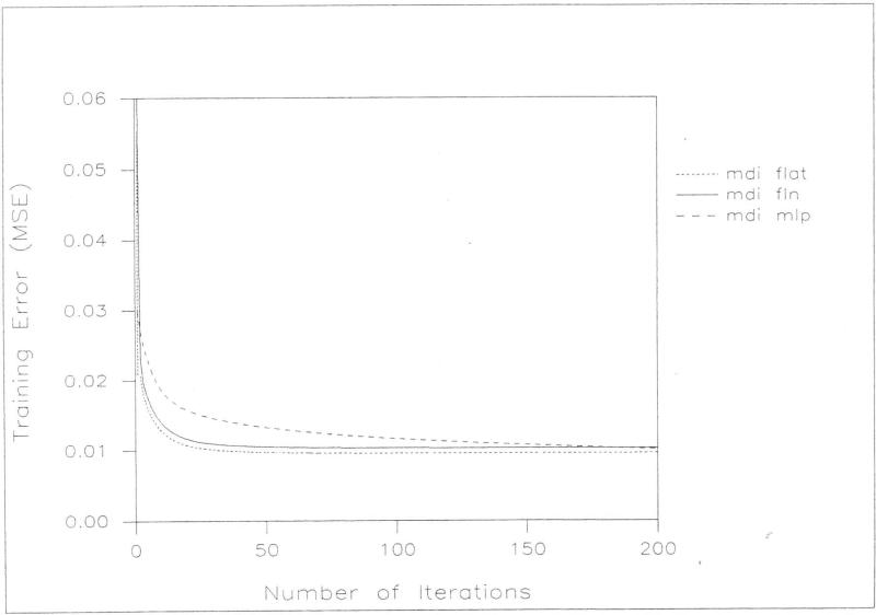
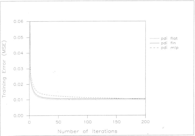
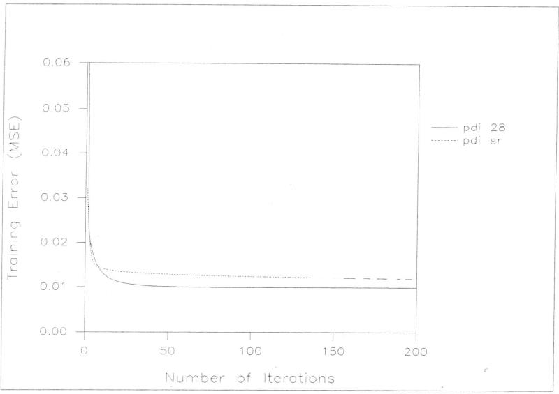
All of the models fit well to the data used in their construction. The mean-squared error (MSE) was computed by averaging the squares of the differences between actual outcome and predicted outcome for all inputs in the training data set. Among the neural network models, the flat net fit slightly better for both MDI and PDI prediction on the basis of a comparison of mean square error at 200 iterations. Among the three neural network models, the flat net required the least training time and the MLP the greatest time to achieve an acceptable training error. The flat net model for predicting MDI achieved a training error of 0.01 within only 50 iterations while neither of the other networks had achieved that training error by the 200 iteration maximum. The flat net model for predicting POI achieved a training error of 0.0125 within only five iterations while the FLN required ten and the MLP over 50 iterations to achieve that training error. Figures [2] and [3] graphically display the results of the training experiments.
Figure 2.
A comparison of MDI training error (MSE) and the number of iterations for flat net (mdi flat), functional-link net (mdi fln) and feed forward MLP (mdi mlp) .
Figure 3.
A comparison of PDI training error (MSE) and the number of iterations for flat net (pdi flat), functional-link net (pdi fin) and feed forward MLP (pdi mlp).
3.1. Prediction Error
Prediction error for each of the various models was determined by computing a percent error using the target outcome and the predicted outcome within each of the trial sets. Comparisons of models were made by using pairwise t-test. In order to reduce the effects of sampling, we performed this test in each of three trials in which 200 data records of the 331 were used for training and the remaining records used for testing. For each trial and for each of PDI and MDI prediction data records missing any values required for the trial were eliminated, resulting in slightly different data set size among the six experiments.
Among the baseline neural network models, the MLP generally provided the lowest prediction error and the flat net the highest (Table [3]). The flat net performed at least as well as the other network models in two of the three trial sets for PDI. The MLP outperformed the other network models in the other PDT trial. In the MDI trials, the MLP was better for two of the trial data sets, and there was no significant difference in performance in the other trial.
Table 3.
PERCENT PREDICTION ERROR: Flat Net, Feed Forward MLP and Functional-link Net (FLN) (28 input variables)
| Flat Net | FLN | Feed Forward MLP | ||||||||||||
|---|---|---|---|---|---|---|---|---|---|---|---|---|---|---|
| N | Mean1 | SD | Min | Max | Mean1 | SD | Min | Max | Mean1 | SD | Min | Max | ||
| MDI | Set1 | 82 | −1.8 | 39.3 | −268.6 | 52.5 | −2.3 | 43.6 | −262 | 53.8 | 3.9 | 20.4 | −41.2 | 72.5 |
| Set2 | 88 | 6.6 | 14.7 | −26.0 | 54.1 | −4.0 | 17.1 | −45.9 | 49.3 | −.7 | 16.0 | −48.8 | 49.8 | |
| Set3 | 81 | 5.0 | 18.1 | −34.8 | 66.7 | 6.3 | 16.8 | −28.1 | 59.1 | −1.3 | 20.2 | −78.8 | 50.7 | |
| MEAN | 3.3 | 24.0 | 0.0 | 25.8 | .63 | 18.87 | ||||||||
| PDI | Setl | 82 | −1.6 | 24.3 | −131.0 | 36.7 | −9.1 | 36.1 | −193.1 | 35.8 | 1.4 | 19.9 | −55.3 | 70.0 |
| Set2 | 88 | 5,4 | 15.2 | −26.6 | 37.8 | 1.9 | 16.4 | −29.2 | 35.9 | 1.7 | 15.9 | −41.2 | 32.2 | |
| Set3 | 81 | −1.2 | 21.9 | −67.5 | 65.1 | 4.0 | 20.3 | −63.7 | 50.6 | −3.4 | 22.5 | −105.2 | 42.4 | |
| MEAN | 0.9 | 20.5 | −1.1 | 24.3 | −0.1 | 19.4 | ||||||||
Mean % error
The stepwise multiple linear regression model identified different sets of significant variables in each of the tree trials for each of PDI and MDI outcomes (Table [2]). Using these sets of regression-selected variables, “statistically” enhanced flat net models were constructed. Although there was no significant difference in prediction error between the multiple linear regression model and the statistically enhanced flat net model, the tlat net produced significantly lower variance predictions (p < 0.0001) in all three MDI trials and two of the three PDI trials (p < 0.05) (Table [4]). The flat net also performed better for the prediction of extreme outcomes.
Table 4.
PERCENT PREDICTION ERROR: Stepwise Regression and Flat Net (using the Stepwise Regression Selected Variables)
| Stepwise Regression | Flat Net | ||||||||||||
|---|---|---|---|---|---|---|---|---|---|---|---|---|---|
| Mean1 | SD | Mean2 | SD | Min | Max | Mean1 | SD | Mean2 | SD | Min | Max | ||
| MDI | Set1 | −12.6 | 50.4 | 23.4 | 46.3 | −338.8 | 28.9 | 0.3 | 19.5 | 14.8 | 12.6 | −48.8 | 65.7 |
| Set2 | −4.7 | 22.4 | 15.8 | 16.5 | −126.6 | 29.5 | 0.6 | 18.0 | 14.1 | 11.1 | −3.9 | 52.6 | |
| Set3 | −8.2 | 39.9 | 20.2 | 35.4 | −283.5 | 32.2 | 0.9 | 20.9 | 15.5 | 13.8 | −55.8 | 70.6 | |
| MEAN | −8.5 | 37.6 | 19.8 | 32.7 | 0.6 | 19.5 | 14.8 | 12.5 | |||||
| PDI | Set1 | −8.4 | 46.5 | 22.0 | 41.8 | −343.6 | 37.0 | −2.9 | 21.7 | 16.3 | 14.5 | −58.9 | 73.6 |
| Set2 | −5.3 | 20.1 | 15.7 | 13.4 | −74.9 | 34.7 | 1.1 | 19.0 | 15.1 | 11.5 | −57.1 | 39.1 | |
| Set3 | −3.6 | 31.7 | 19.2 | 25.4 | −175.5 | 37.9 | −2.2 | 21.4 | 16.0 | 14.3 | −49.5 | 60.8 | |
| MEAN | −5.8 | 32.8 | 15.7 | 41.8 | −1.3 | 20.7 | 15.8 | 14.5 | |||||
Mean % error
Mean % absolute error
When we compared the prediction performance of the baseline (28 variable) flat net model and the statistically enhanced flat net model, the statistically enhanced flat net model performed significantly better than the baseline flat net model for two of the three MDI trials (p < 0.002) with no significant difference in performance in the other trial. There was no significant difference in performance in any of the three PDI trials. Again, the statistically enhanced flat net model generally produced lower variance predictions than the baseline flat net model. See Table [5].
Table 5.
PERCENT PREDICTION ERROR: Flat Net with All 28 Variables and with Stepwise Regression Selected Variables
| Stepwise Regression Selected Variables | All Variables (28) | ||||||||||||
|---|---|---|---|---|---|---|---|---|---|---|---|---|---|
| Mean1 | SD | Mean2 | SD | Min | Max | Mean1 | SD | Mean2 | SD | Min | Max | ||
| MDI | Set1 | 0.3 | 19.5 | 14.8 | 12.6 | −48.8 | 65.7 | −1.8 | 39.3 | 20.5 | 33.6 | −268.6 | 52.5 |
| Set2 | 0.6 | 18.0 | 14.1 | 11.1 | −43.9 | 52.6 | 6.6 | 14.7 | 12.6 | 9.9 | −26.0 | 54.1 | |
| Set3 | 0.9 | 20.9 | 15.5 | 13.8 | −55.8 | 70.6 | 5.0 | 18.1 | 13.6 | 12.8 | −34.8 | 66.7 | |
| MEAN | 0.6 | 19.5 | 14.8 | 12.5 | 3.3 | 24.0 | 15.6 | 18.8 | |||||
| PDI | Set1 | −2.9 | 21.7 | 16.3 | 14.5 | −58.9 | 73.6 | −1.6 | 24.3 | 16.6 | 17.8 | −131.0 | 36.7 |
| Set2 | 1.1 | 19.0 | 15.1 | 11.5 | −57.1 | 39.1 | 5.4 | 15.2 | 13.1 | 9.2 | −26.6 | 37.8 | |
| Set3 | −2.2 | 21.4 | 16.0 | 14.3 | −49.5 | 60.8 | −1.2 | 21.9 | 15.8 | 15.0 | −67.5 | 65.1 | |
| MEAN | −1.3 | 20.7 | 15.8 | 13.4 | 0.9 | 20.5 | 15.2 | 14.0 | |||||
Mean % error
Mean % absolute error
3.2 Importance of Predictor Variables
There was substantial agreement on included and excluded variables among the three stepwise multiple linear regression models (Table [2]). However, attempts to relate the contribution of a variable to the predictive ability of a neural network model via the magnitude of its associated link weights were inconclusive. Although a precise interpretation of the relevance of link weight magnitudes in neural networks has yet to be given, it seems reasonable that link weights of relatively small magnitudes (approaching zero) in a flat net architecture imply that the connecting input has very little bearing on the process outcome. Our results neither support nor reject this conclusion.
4. Discussion
The flat neural network model performed well as compared to the regression model (Table [4]). In addition to less variation in prediction error, the flat net also displayed robust learning in the presence of extraneous inputs. This characteristic is advantageous when there is not much knowledge about the influential factors on a process outcome.
Perhaps the most interesting finding in our work was the consistency with which both the statistical modeling approach and the neural network modeling approach rejected the introduction of nonlinear elements in this particular setting. The flat network with no enhancements generally performed as well as both the FLN and the MLP. This might be considered unexpected because the flat network is a special case of both the FLN and the MLP in which the nonlinear elements, enhanced inputs and hidden layers, respectively, are removed. The lack of improvement of performance that results from the inclusion of nonlinear model elements strongly suggests that there is a simple linear relationship between the input data and output data of the test data sets.
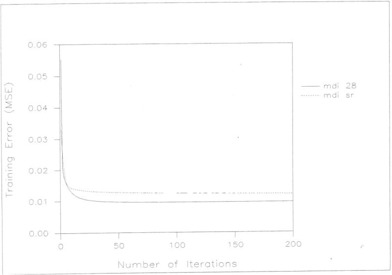
The results of the comparison of the baseline flat network model and the statistically enhanced flat net model were inconsistent in that in half of the trials the enhanced network was superior and in the other half there was no significant difference (Table [5]). Although the baseline flat network fits the data slightly better in training (Figures [4] and [5]) , training of the enhanced flat net required 50% less computational overhead due to of the fewer number of variables involved. Equally importantly, the enhanced flat net requires less neural computation in post-training work. In conventional neural computation, relevant inputs are selected by trial and error through a process of training a network and then analyzing the results to determine which inputs can be eliminated. This process is tedious and limited because redundancies among inputs cannot be isolated by this technique. As we have shown, regression can be used to select relevant inputs in a less tedious way .
Figure 4.
A comparison of MDI training error (MSE) and the number of iterations for flat net with stepwise regression selected variables (mdi sr) and all 28 variables (mdi 28).
Figure 5.
A comparison of PDI training error (MSE) and the number of iterations for flat net with stepwise regression selected variables (pdi sr) and all 28 variables (pdi 28).
Examination of the relative magnitudes of the link weights in the trained networks does not reveal a strong consistency in selection of the same variables as significant to the predicted outcome. The results of the linear regression model in this regard are more consistent. This is disappointing because it casts doubt on the possibility that direct analysis of link weights could supplant regression as a method for selecting relevant input variables.
With the advent of improved medical care for very low birth weight infants and those with BPD, more such infants are surviving and it is anticipated that most will probably enter childhood and early adulthood with significant medical and developmental problems. Because BPD is a relatively new disease, the long term outcome remains unknown. Thus, any technology that can help accurately predict the clinical outcome for such infants will improve overall clinical management. As we progress with our study we hope to continue to combine the strengths of statistical and neural network methods to predict second and third year outcomes of these children using demographic, medical and historical behavioral variables.
Acknowledgements
This study was supported in part by grants from the NIH RO1-HL38193 and MCJ390592. We wish to thank Ms. Jie Huang for her assistance in the statistical analysis.
Contributor Information
Toyoko S Yamashita, Departments of Pediatrics and Epidemiology & Biostatistics, Case Westem Reserve University School of Medicine, Cleveland, Ohio 44106 U.S.A. tsy@po.cwru.edu
Isaac F. Nuamah, Biostatistics Unit, University of Pennsylvania Cancer Center, Philadelphia, Pennsylvania 19104 U.S.A. nuamah@a1.mscf.upenn.edu
Philip A. Dorsey, Departments of Electrical Engineering and Pediatrics, Case Western Reserve University, Cleveland, Ohio 44106 U.S.A.
Seyed M. Hosseini-Nezhad, Department of Electrical Engineering, Case Western Reserve University, Cleveland, Ohio 44106 U.S.A.
Roger A. Bielefeld, Department of Epidemiology and Biostatistics, Case Western Reserve University School of Medicine, Cleveland, Ohio 44106 U.S.A. rab@hal.cwru.edu
Edward F. Kerekes, Department of Pediatrics, Case Western Reserve University School of Medicine, Cleveland, Ohio 44106 U.S.A.
Lynn T. Singer, Department of Pediatrics, Case Western Reserve University School of Medicine, Cleveland, Ohio 44106 U.S.A.
References
- 1.Baxt W. Use of an artificial neural network for the diagnosis of myocardial infarction. Annals of Internal Medicine. 1991;115:843–848. doi: 10.7326/0003-4819-115-11-843. [DOI] [PubMed] [Google Scholar]
- 2.Brei man L, Friedman JH, Olshen RA, Stone CJ. Classification and Regression Trees. Wadsworth; Belmont, California: 1984. [Google Scholar]
- 3.Cleveland WS. Robust locally weiglued regression and smoothing scatter plots. J. Amer. Stat. Assoc. 1979;74:828–836. [Google Scholar]
- 4.Davis GE, Lowell WE, Davis GL. A neural network that predicts psychiatric length of stay. M.D. Computing. 1993;2:87–92. [PubMed] [Google Scholar]
- 5.Friedman JH, Wright MH. A nested partitioning procedure for manerical multiple integration. ACM Trans. Math. Software. 1981;7:76–92. [Google Scholar]
- 6.Friedman JH. Multivariate adaptive regression splines (with discussion) Ann. Stat. 1991;19:1–141. [Google Scholar]
- 7.Hastie TJ, Tishirani RJ. Generalized Additive Models. Chapman and Hall; London: 1990. [Google Scholar]
- 8.Hornik K, Stinchcombe M, White H. Multilayer feedforward networks are universal approximators. Neural networks. 1989;2:359–366. [Google Scholar]
- 9.Hosmer DW, Lemeshow S. Applied Logistic Regression. John Wiley and Sons; New York: 1989. [Google Scholar]
- 10.Hosseini-Nezhad SM, Yamashita TS, Bielefeld RA, Krug SE, Pao Y-H. Detennination of lnterhospital Transport Mode by a Neural Network. Computers and Biomedical Research. doi: 10.1006/cbmr.1995.1022. (under review) [DOI] [PubMed] [Google Scholar]
- 11.Hosseini-Nezhad SM, S Yamashita T, Blumer JL, Pao Y-H. A Neural Network Approach to PICU Medical Infonnation Utilization. Bedside Computing in the 90's. 1991;50 [Google Scholar]
- 12.Huber PJ. Projection pursuit (with discussion) Ann. Stat. 1985;13:435–475. [Google Scholar]
- 13.Lachenbruch PA. Discriminant Analysis. Hafner Press; New York: 1975. [Google Scholar]
- 14.Pao Y-H. Adaptive Pattern Recognition and Neural Networks. Addison-Wesley; 1989. [Google Scholar]
- 15.Pao Y-H. In Functional-link net: removing hidden/ayers. AI Expert. 1989;4:60–68. [Google Scholar]
- 16.Pao Y-H, Takefuji Y. Functional-link net computing: theory, system, architecture and fwzctionalities. Computer. 1992;5:76–79. [Google Scholar]
- 17.Riley BD. Statistical aspects of neural networks, Proceeding of the European Statistical Seminar. Chapman and Hall; London: 1993. [Google Scholar]
- 18.Singer L, Martin R, Hawkins S, Benson-Szekely L, Yamashita T, Carlo W. Oxygen desaturation complicates feeding of bronchopulmonary dysplasia infants in the home environment. Pediatrics. 1992;90:380–384. [PMC free article] [PubMed] [Google Scholar]
- 19.Singer L, Yamashita T, Hawkins S, Cairns D, Kliegman R. Incidence of Intraventricular Hemorrhage in Cocaine-Exposed, Very Low Birthweight Infants. J. Ped. 1994;124:765–771. doi: 10.1016/s0022-3476(05)81372-1. [DOI] [PMC free article] [PubMed] [Google Scholar]
- 20.Singer L, Yamashita T, Hawkins S, Bruening P, Davillier M. Fathers of very low birthweight infants: Distress, coping and changes over time. Abstracts of the SRCD. 1993;9:598. [Google Scholar]
- 21.Singer L, Yamashita T, Hawkins S, Collin M, Baley J. Bronchopulmonary dysplasia and cocaine-exposure predict poorer motor outcome in very low birthweight infants. Pediatric Res. 1993;33:276A. [Google Scholar]
- 22.Smith PL. Splines as a useful and convenient statistical tool. Amer. Stat. 1979;33:57–62. [Google Scholar]
- 23.Tu JV, Guerriere MRJ. Use of a neural network as a predictive instrument for length of stay in the intensive care unit following cardiac surgery. Computers and Biomedical Research. 1993;26:220–229. doi: 10.1006/cbmr.1993.1015. [DOI] [PubMed] [Google Scholar]
- 24.Yamashita TS, Ganesh P, Krug SE. A Neural Network based pediatric transport scoring System. Pediatric and Perinatal Epidemiology. 1991;5:A2. [Google Scholar]
- 25.Yamashita TS, Hosseini-Nezhad SM, Krug SE. A Functional-link net approach to pediatric interhospital transport mode determination. In: Lun KC, et al., editors. “MEDINFO 92”. Elsevier Science Publishers B. V.; North-Holland: 1992. p. 672. [Google Scholar]
- 26.Veselis RA, Reinsel R, Sommer S, Carlon G. Use of neural network analysis to classify electroencephalographic pattems against depth of midazolam sedation in intensive care unit patients. Journal of Clinical Monitoring. 1991;7:259–267. doi: 10.1007/BF01619271. [DOI] [PubMed] [Google Scholar]


