Learning a Dictionary of Shape Epitomes with Applications to Image Labeling

Abstract

The first main contribution of this paper is a novel method for representing images based on a dictionary of shape epitomes. These shape epitomes represent the local edge structure of the image and include hidden variables to encode shift and rotations. They are learnt in an unsupervised manner from groundtruth edges. This dictionary is compact but is also able to capture the typical shapes of edges in natural images. In this paper, we illustrate the shape epitomes by applying them to the image labeling task. In other work, described in the supplementary material, we apply them to edge detection and image modeling.

We apply shape epitomes to image labeling by using Conditional Random Field (CRF) Models. They are alternatives to the superpixel or pixel representations used in most CRFs. In our approach, the shape of an image patch is encoded by a shape epitome from the dictionary. Unlike the superpixel representation, our method avoids making early decisions which cannot be reversed. Our resulting hierarchical CRFs efficiently capture both local and global class co-occurrence properties. We demonstrate its quantitative and qualitative properties of our approach with image labeling experiments on two standard datasets: MSRC-21 and Stanford Background.

1. Introduction

In this paper, we propose a novel representation for local edge structure based on a dictionary of shape epitomes, which were inspired by [12]. This dictionary is learnt from annotated edges and captures the mid-level shape structures. By explicitly encoding shift and rotation invariance into the epitomes, we are able to accurately capture object shapes using a compact dictionary of only five shape epitomes. In this paper, we explore the potential of shape epitomes by applying them to the task of image labeling. Most modern image labeling systems are based on Conditional Random Fields (CRFs) [18, 20] for integrating local cues with neighborhood constraints. Image segments are typically represented in the pixel domain [9, 17, 26], or in the domain of superpixels (a region of pixels with uniform statistics) [6, 7, 10, 11, 21, 23].

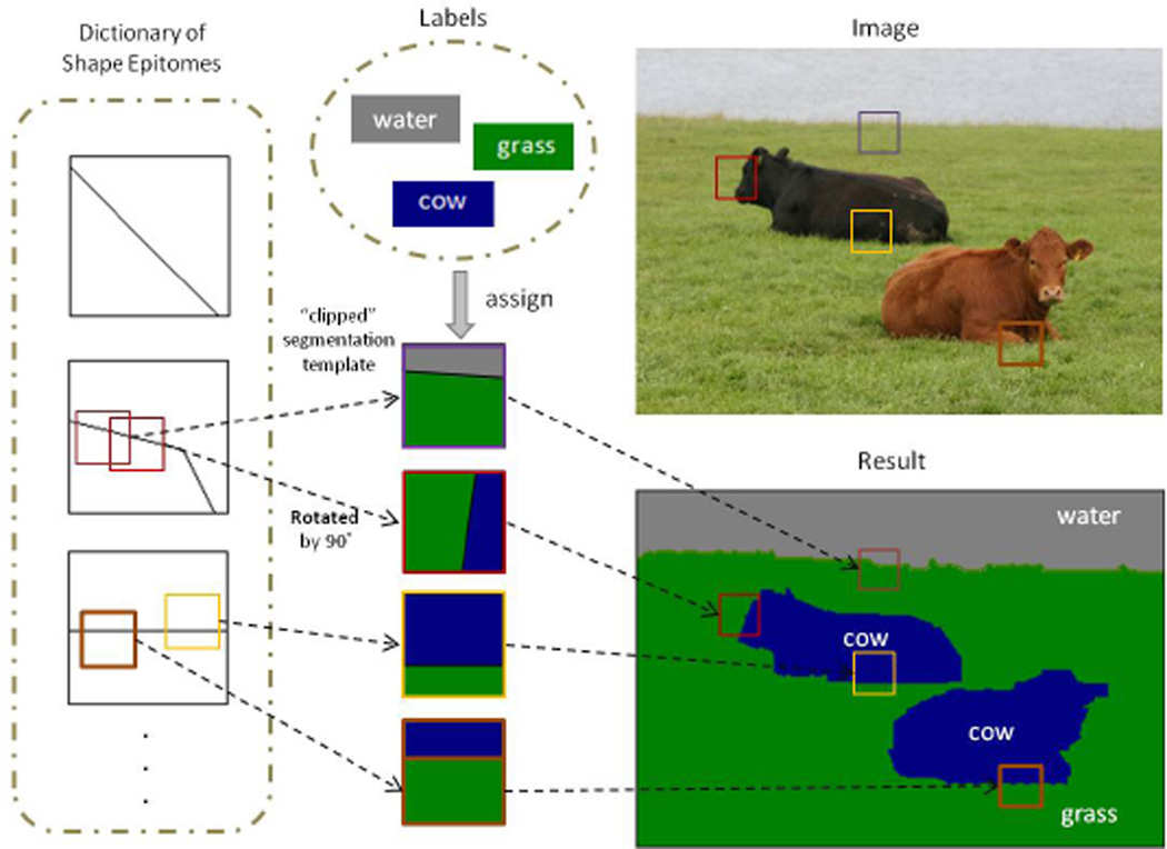
One motivation for shape epitomes was the success of segmentation templates for image labeling [27]. These templates also represent the local edge structure but differ from pixels and superpixels because they represent typical edges structures, such as L-junctions, and hence provide a prior model for edge structures. Each patch in the image was encoded by a particular segmentation template with semantic labels assigned to the regions specified by the template, as illustrated in Fig. 1. Segmentation templates, like superpixels, have computational advantages over pixel-based approaches by constraining the search process and also allow enforcing label consistency over large regions. Compared to superpixels, segmentation templates do not make early decisions based on unsupervised over-segmentation and, more importantly, explicitly enumerate the possible spatial configurations of labels making it easier to capture local relations between object classes. See Table 1 for a comparison summary.

Figure 1.

Proposed dictionary of Shape Epitomes in the context of image labeling. Segmentation templates are generated from the shape epitomes, by specifying the values of the hidden variables. Image labels are assigned to the regions within the templates, and thus the local relationship between object classes is explicitly modeled. Note the rotation and shift-invariance illustrated in the second and third shape epitome, respectively.

Table 1.

General comparison between representations from the aspects of Computation, Flexibility (better align with object shapes), Long-Range consistency, and ability to Explicitly model the local configuration of objects. We improve the flexibility of template-based representation by learning a dictionary of shape epitomes.

	Pixel	Superpixel	Template
Computation	−	+	+
Flexibility	+	+	+
Long-Range	−	+	+
Explicit Configuration	−	−	+

But those segmentation-templates [27] have limitations. Firstly, they were hand-specified. Secondly, there were not invariant to shift and rotation which implies that a very large number of them would be needed to give an accurate representation of edge structures in the images (Zhu et al [27] used only thirty segmentation-templates which meant that they could only represent the edges very roughly).

Each shape epitome can be thought of a set of segmentation-templates which are indexed by hidden variable corresponding to shift and rotation. More precisely, a shape epitome consists of two square regions one inside the other. The hidden variable allows the inner square region to shift and rotate within the the bigger square, as shown in Fig. 1. The hidden variable specifies the shift and rotation. In the current paper, each shape epitome corresponds to 81 × 4 = 324 segmentation-templates. Hence, as we will show, a small dictionary of shape epitomes is able to accurately represent the edge structures (see Sec. 4.3.1). Intuitively the learned dictionary captures generic mid-level shape-structures, hence making it transferable across datasets. By explicitly encoding shift and rotation invariance, our learned epitomic dictionary is compact and only uses five shape epitomes. We also show that shape epitomes can be generalized to allow the inner square to expand which allow the representation to deal with scale (see Sec. 4.3.4).

We propose shape epitomes as a general purpose representation for edge structures (i.e. a mid-level image description). In this paper we illustrate them by applying them to the image labeling task. In the supplementary material we show how they can be also used for edge detection and for local appearance modeling. For image labeling, we consider three increasingly more complex models, which adapt current CRF techniques for shape epitomes. We use patches at a single fine resolution whose shape is encoded by a segmentation template (i.e. a shape epitome with hidden variable specified). The patches are overlapping, thus allowing neighbors to directly communicate with each other and find configurations which are consistent in their area of overlap (Model-1). We explore two enhancements of this basic model: Adding global nodes to enforce image-level consistency (Model-2) and also further adding an auxiliary node to encourage sparsity among active global nodes, i.e., encourage that only few object classes occur within an image (Model-3). We conduct experiments on two standard datasets, MSRC-21 and Stanford Background, obtaining promising results.

Related work

Our model is based on the success of several works. First, the ability to generate an image from a condensed epitomic representation [12]. We leverage on this idea to learn a dictionary of shape epitomes. Each segmentation template is generated within a shape epitome. This encodes the shift-invariance into the dictionary, since a segmentation template is able to move within a shape epitome. Besides, we encode rotation invariance by allowing the shape epitome to rotate by 0, 90, 180, and 270 degrees.

Second, the potential of using template-based representation and overlapped patches. It has been shown that learning the generic patterns capturing statistics over large neighborhoods can be beneficial for image denoising [24] and image labeling [15]. Besides, finding the mutual consensus between neighboring nodes by using overlapped patches [28] has shown to be effective. Similar ideas have been applied to image labeling [16]. However, they did not learn a dictionary for object shapes.

Third, the power of introducing simple global nodes for image labeling. Ladicky et al. [19] introduced global nodes that can take values from the predefined label set L and a “free” label. There is no energy cost, when the global node takes the free label. Gonfaus et al. [8] proposed a harmony model to generalize the idea by allowing the global node to take labels from the power set of L. However, it is computationally challenging to find the most probable state for the global node from the power set. Then, Lucchi et al. [22] proposed the Class Independent Model (CIM) to decompose the global node into |L| global nodes. Our model moves further based on the CIM by encoding the image-level co-occurrence, and adding an auxiliary node to encourage the sparsity of active global nodes, similar to [4].

Structure

Sec. 2 describes our method of learning a dictionary of shape epitomes, and Sec. 3 describes our model based on CRF. Experimental results are discussed in Sec. 4.

2. Learning a dictionary of shape epitomes

In this section, we present our algorithm for learning the dictionary of shape epitomes from annotated images.

To learn the generic dictionary, we use the BSDS500 dataset [1], which provides ground truth of object boundaries. Given that, we extract M × M patches around the shape boundaries (called shape patches). We cluster these shape patches using affinity propagation [5] to build our shape epitomes (note that the size of shape patches is the same as that of shape epitomes). The segmentation templates are of smaller size m × m (m < M) than the shape epitomes, and are generated as sub-windows of them. By generating the segmentation template from a larger shape epitome, we are able to explicitly encode shift-invariance into the dictionary, as illustrated in Fig. 1. Therefore, one shape epitome compactly groups many segmentation templates which are shifted versions of each other.

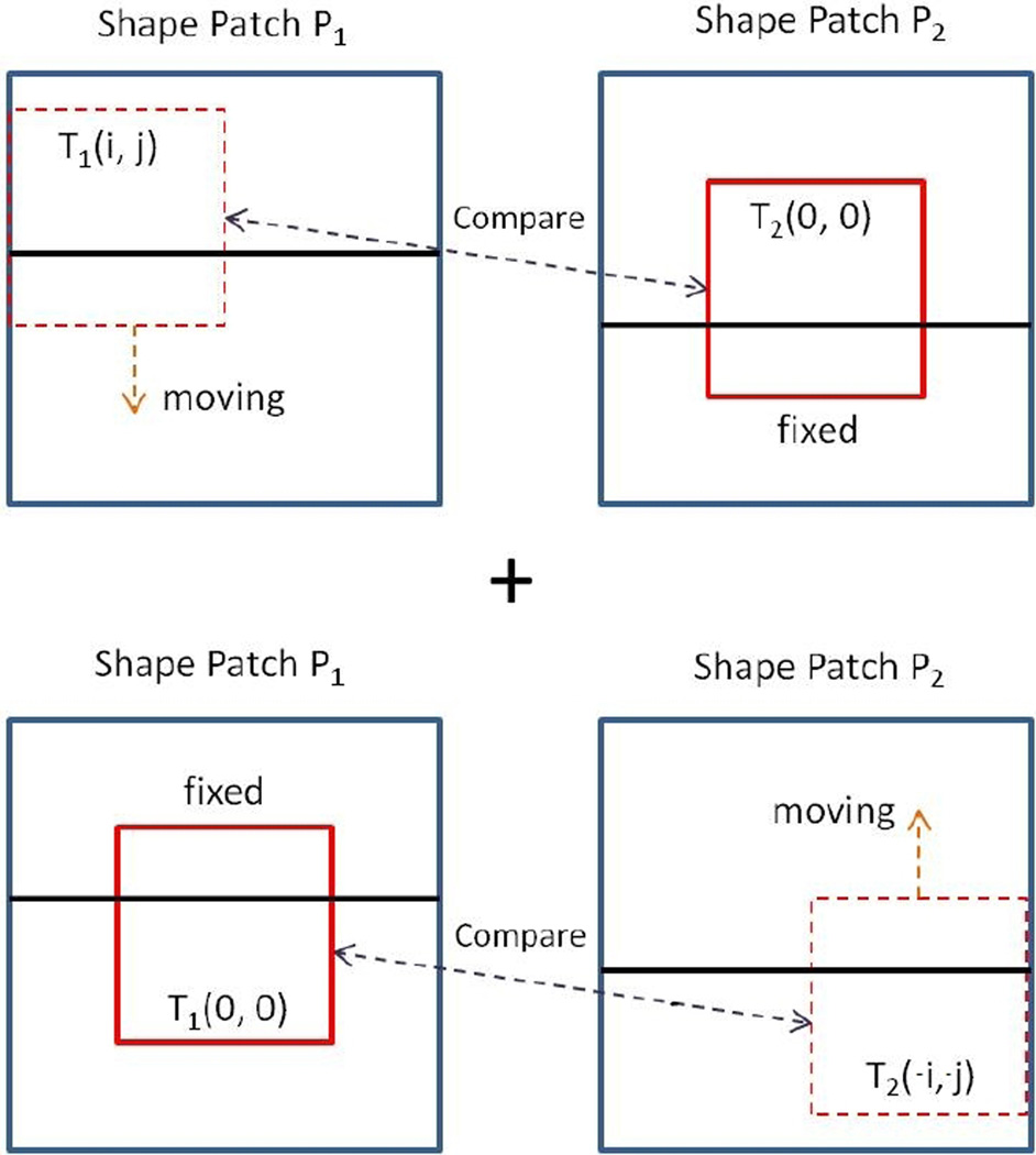
Clustering by affinity propagation requires a similarity measure F (P₁, P₂) between two M × M shape patches P₁ and P₂. We induce F (P₁, P₂) from another similarity measure F_T (T₁, T₂) between two m × m segmentation templates T₁ and T₂ extracted from P₁ and P₂, respectively. Specifically, let T (i, j) denote the segmentation template extracted from P and centered at (i, j), with (0, 0) being the center of P. We define the similarity between the two shape patches P₁ and P₂ to be

$$F(P_1,P_2)=\underset{\frac{m-M}{2}\le i,j\le \frac{M-m}{2}}{\text{max}}\frac{1}{2}[F_T(T_1(i,j),T_2(0,0))+F_T(T_1(0,0),T_2(-i,-j))],$$ (1)

as illustrated in Fig. 2. We employ the covering of the template T₁ by the template T₂ [1] as the similarity measure F_T (T₁, T₂) between them:

$$F_T(T_1,T_2)=\frac{1}{|T_2|}\sum _{r_2\in T_2}|r_2|\underset{r_1\in T_1}{\text{max}}\frac{|r_1\cap r_2|}{|r_1\cup r_2|},$$

where r₁ and r₂ are the regions in templates T₁ and T₂, respectively, and |r| is the area of region r. Note that F_T (T₁, T₂) and consequently F (P₁, P₂) range from 0 (no similarity) to 1 (full similarity).

Figure 2.

The similarity measure between two shape patches. The optimal value of shift variables (i, j) is shown for this example.

Directly applying affinity propagation results in many similar shape epitomes because simple horizontal or vertical boundaries are over-represented in the training set. We follow [13] and grow the dictionary incrementally, ensuring that each newly added shape epitome is separated from previous ones by at least distance t, as follows:

1. Clustering. Apply affinity propagation to find one shape epitome that contains the most members (i.e., the largest cluster) in current training set.

2. Assigning. For each shape patch in training set, assign it to the shape epitome found in step 1, if their distance, defined as 1 − F (P₁, P₂), is smaller than t.

3. Update. Remove the shape patches that are assigned to the shape epitome from the current training set.

4. Repeat until no shape patch is left in the training set.

3. Adapting CRFs for segmentation templates

Having learned the dictionary of shape epitomes, we now proceed to show how we can build models for image labeling on top of it. We propose three models by adapting current CRF models to the template-based representation.

The problem of image labeling in this context can be formulated as follows. Given an image I, we represent it by a set of overlapped m × m patches. The goal is to encode each patch by a segmentation template, and by assigning labels (from a categorical set L) to each region in the segmentation template. Specifically, the labeling assignment x is represented by both segmentation template and labels. That is, x = {x_i}_i∈𝒱 with x_i = {s_i, l_i}, where 𝒱 is the set of patches, s_i and l_i denote the type of segmentation template and object labeling, respectively. Note that l_i is a vector, whose length is the number of regions within the segmentation template. For example, l_i = (cow, grass) means that label cow and label grass are assigned to the first region and second region within segmentation template s_i. We call our models SeCRF, short for Shape epitome CRF.

3.1. Model 1: One-level SeCRF

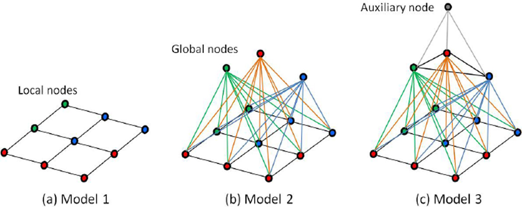
We first introduce a flat model, which is represented by a graph with a single layer 𝒢 = {𝒱_l, ℰ_l}, as shown in Fig. 3(a). Each node corresponds to a patch region, and it is encoded by both the type of segmentation template and the labels assigned to it. The image region represented by node i (i.e., i-th patch) is denoted by R (i).

Figure 3.

Adapting CRFs for segmentation templates. (a) Model 1 uses only a single layer of local nodes. (b) Model 2 adds global nodes to encode global consistency, similar to [22] (but the energy value is soft in our model). (c) Model 3 encodes the pairwise co-occurrence between global nodes, and adds an auxiliary node to encourage the sparsity of active global nodes.

The energy of x given image I is given by:

$$E(\mathit{x}|I)=E_1(\mathit{x};{\alpha }_1)+E_2(\mathit{x};{\alpha }_2)+E_3(\mathit{s};{\alpha }_3)+E_4(\mathit{l};{\mathit{\alpha }}_{\mathbf{4}})+E_5(\mathit{x};{\mathit{\alpha }}_{\mathbf{5}})$$ (2)

where α is the model parameters. Note we suppress the dependency on the image I in subsequent equations. Each energy term is defined below.

The first term E₁ (x; α₁) is the data term which accumulates the pixel features with respect to certain type of segmentation template and labels assigned to the corresponding regions. We set E₁ (x; α₁) = −α₁ ∑_i∈𝒱l ψ₁ (x_i), and

$${\psi }_1(x_i)=\frac{1}{|R(i)|}\sum _{p\in R(i)}\text{log}\hspace{1em}\mathit{\text{Pr}}(x_i^p|I)$$

where we define $x_i^p$ as the labeling of pixel p in the region of segmentation template s_i. The value $\mathit{\text{Pr}}(x_i^p|I)$ is computed by a strong classifier with features (e.g., filter bank responses) extracted within a region centered at position p.

The second term is used to encourage the consistency between neighboring nodes in their area of overlap. For a pixel that is covered by both node i and j, we encourage node i to assign the same label to it as node j. The consistency is defined by using the Hamming distance:

$$E_2(\mathit{x};{\alpha }_2)=-{\alpha }_2\sum _{(i,j)\in {ℰ}_l}{\psi }_2(x_i,x_j)$$

where

$${\psi }_2(x_i,x_j)=\frac{1}{|O(i,j)|}\sum _{p\in O(i,j)}\delta (x_i^p=x_j^p)$$

where O (i, j) is the overlapped region between nodes i and j, and $\delta (x_i^p=x_j^p)=1$ if $x_i^p=x_j^p$, and zero, otherwise. In our experiments, we use 4-neighborhood.

The third term encodes the generic prior of segmentation templates. Specifically, we binarize the type of s_i to be either 1, meaning that it contains some type of shapes, or 0, meaning that it contains no shape.

$$E_3(\mathit{s};{\alpha }_3)=-{\alpha }_3\sum _{i\in {𝒱}_l}\text{log}\hspace{1em}\mathit{\text{Pr}}(s_i)$$

The fourth term E₄ (x; α₄) is used to model the co-occurrence of two object classes within a segmentation template. Note that parameter α₄ is a 2-D matrix, indexed by u and υ, ranging over the label set L.

$$E_4(\mathit{l};{\mathit{\alpha }}_4)=-\sum _{i\in {𝒱}_l}\sum _{u,\upsilon =1,\dots ,|L|}{\alpha }_4(u,\upsilon ){\psi }_4(u,\upsilon ,{\mathit{l}}_i)$$

where |L| is the total number of object classes, and ψ₄ (u, υ, l_i) is an indicator function which equals one when both object classes u and υ belong to l_i.

The fifth term E₅ (x; α₅) models the spatial relationship between two classes within a segmentation template. We model only the ”above” relationship. For example, we encourage sky to appear above road, but not vice versa.

$$E_5(\mathit{x};{\mathit{\alpha }}_5)=-\sum _{i\in {𝒱}_l}\sum _{u,\upsilon =1,\dots ,|L|}{\alpha }_5(u,\upsilon ){\psi }_5(u,\upsilon ,x_i)$$

where ψ₅ (u, υ, x_i) is an indicator function which equals one when object class m is above class n within a certain segmentation template. Note that for some segmentation template that does not have the ”above” relationship (e.g., a template with vertical boundary), this term is not used.

3.2. Model 2: Two-level SeCRF

Motivated by the Class Independent Model (CIM) in [22], we add |L| independent global nodes {𝒱_g} to enforce image-level consistency, as shown in Fig. 3(b). A global node encodes the absence or presence of a object class in the image (i.e., y_i ∈ {0, 1}, ∀i ∈ 𝒱_g), and it is densely connected to every local node. We denote the set of edges connecting global nodes and local nodes as {ℰ_lg}, and then labeling assignment x = {{x_i}_i∈𝒱l ∪ {y_i}_i∈𝒱g}. An extra global-local energy term is added to Equation 2 with each global node y_j having a 2-D matrix parameter ${\mathbf{\alpha }}_6^j$:

$$E_6(\mathit{x};{\mathit{\alpha }}_6)=-\sum _{(i,j)\in {ℰ}_{lg}}\sum _{u=1}^{|L|}\sum _{\upsilon =0}^1{\alpha }_6^j(u,\upsilon ){\psi }_6(u,\upsilon ,x_i,y_j)$$

where

$${\psi }_6(u,\upsilon ,x_i,y_j)=\{\begin{array}{cc}\frac{1}{|R(i)|}\sum _{p\in R(i)}\delta (x_i^p=u),\hfill & \text{if}{y}_j=\upsilon \hfill \\ 0,\hfill & \text{otherwise}\hfill \end{array}$$

Note that our Model 2 differs from CIM in two parts. First, the value of function ψ₆ is proportional to the number of pixels whose labels are u in the node x_i. This formulation is different from the energy cost used in the original CIM, which is either zero or one (i.e., a hard value). On the contrary, we formulate this energy cost as a soft value between zero and one. Second, our local nodes are based on overlapped segmentation templates (not superpixels) so that neighbors can directly communicate with each other. Furthermore, unlike the robust Pⁿ model [14], our penalty depends on the region area within a segmentation template, and thus it is a function of the segmentation template type.

3.3. Model 3: Three-level SeCRF

We further refine Model 2 by adding image-level classification scores to the unary term of global nodes [25]. Specifically, we train |L| SVM classifiers to predict the presence or absence of object classes, following the pipeline of [2]. The unary energy for global nodes is then defined as follows.

$$E_7(\mathit{y};{\alpha }_7)=-{\alpha }_7\sum _{i\in {𝒱}_g}C(y_i|I)$$

where C (y_i|I) is the output of i-th classifier.

The independency among global nodes in Model 2 ignores the co-occurrence between object classes in the image level. Hence, we add edges {ℰ_g} to connect every pair of global nodes, and define an energy term on them:

$$E_8(\mathit{y};{\mathit{\alpha }}_8)=-\sum _{(i,j)=e\in {ℰ}_g}\sum _{u,\upsilon =0}^1{\alpha }_8^e(u,\upsilon )\delta (y_i=u,y_j=\upsilon )$$

where ${\mathbf{\alpha }}_8^e$ depends on the specific edge e = {i, j} that connects two different global nodes, y_i and y_j.

As shown in Fig. 3(c), we also add an auxiliary node 𝒱_a (then, x = {{x_i}_i∈𝒱l ∪ {y_i}_i∈𝒱g ∪ {z_i}_i=𝒱a}). This node favors sparsity among global nodes (similar to [4]) by introducing a set of edges {ℰ_ga} from {𝒱_g} to 𝒱_a. Specifically, 𝒱_a is a dummy node, which can take only one meaningless state. We define an energy term on {ℰ_ga} to encourage only few global nodes to be active as follows.

$$E_9(\mathit{y},z_j;{\alpha }_9)=-{\alpha }_9\sum _{(i,j)\in {ℰ}_{ga}}\delta (y_i=0)$$

where δ (y_i = 0) equals one when the global node y_i is off. This energy term has the effect of biasing the global nodes.

4. Experiments

In this section, we first show the results of learning a dictionary of shape epitomes following the methods described in Sec. 2. We then use this dictionary for image labeling using the SeCRF models of Sec. 3.

4.1. Learned dictionary of shape epitomes

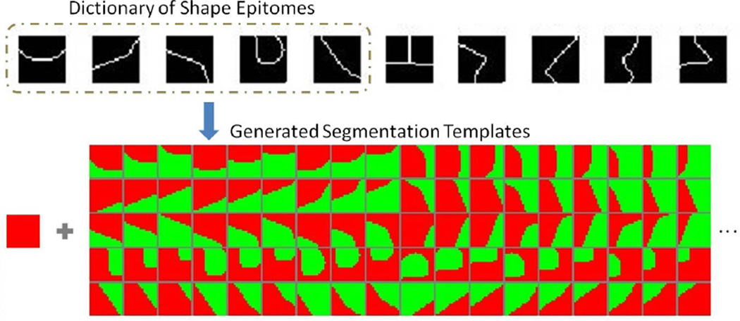
We learn the dictionary of shape epitomes from shape patches extracted from the BSDS500 dataset [1]. In the experiment, we fix the size of a shape patch to be 25 × 25, and the size of segmentation template 17 × 17, namely M = 25 and m = 17. After applying affinity propagation incrementally with distance t = 0.05, the first 10 shape epitomes are shown at the top of Fig. 4.

Figure 4.

Top row: first 10 shape epitomes learned by our method. Bottom: a flat segmentation template (i.e., no shape) and some others generated from the first 5 shape epitomes. Note that some of them are generated from the rotated shape epitomes.

For computational and modeling purposes it is desirable to have a compact dictionary consisting of only few shape epitomes. We have found that the first 5 shape epitomes contain most of the shape patches in the training set of BSDS500, and the cluster size decreases very quickly.

In our setting, a segmentation template is allowed to move within a shape epitome for each horizontal and vertical displacement up to ±4 pixels. We define stride as the step-size for horizontal/vertical displacement. For example, if stride = 4, we can generate 9 templates from each shape epitome, only considering the nine templates T (i, j) ∀i, j ∈ {−4, 0, 4} at all four possible orientations (0, 90, 180 and 270 degrees), ending up with 45 = 9 × 5 templates per epitome. In total, there are 181 (5 × 45 + 1) segmentation templates, including the flat one that contains no shape. On the other hand, if stride = 1, we use every template within a shape epitome, resulting in 1621 (81 × 5 × 4 + 1) segmentation templates.

Using this compact dictionary of 5 shape epitomes suffices to accurately encode the ground truth segmentations in our datasets, as demonstrated in Sec. 4.3.1. As one can observe in Fig. 4, our generated segmentation templates cover the common boundary shapes, such as vertical/horizontal edges, L-junctions, and U-shapes. The learned dictionary thus captures generic mid-level shape-structures and can be used across datasets. We emphasize that we learn it on the BSDS500 dataset and use it unadapted for image labeling on MSRC-21 and Stanford Background datasets.

4.2. Implementation details for image labeling

MAP Inference

We use loopy belief propagation (LBP) to minimize the energy function in Equation 2. We prune the unpromising states by rejecting the unlikely proposals whose E₁ data terms are too high, similar to [27]. We fix the number of states per node to be 100, since in our experiments adding more states only improve the performance marginally at the sacrifice of computation time.

Learning the parameters

We use the same structure-perceptron algorithm [3] as HIM [27], because we would like to have a direct comparison with it by emphasizing on the representation part of our model, not learning.

Fusion of predicted labels

The traditional Conditional Random Field models directly assign an object class label to each pixel in the image. On the contrary, our model uses overlapped patches, and each patch is encoded by a segmentation template and by labels assigned to the regions in the template. The number of patches that will cover the same pixel depends on the size of overlap between patches. We set the overlap size to be (m − 1)/2 pixels in all experiments. To find the labels for every pixel, we fuse the predicted labels for each pixel by letting the patch having the minimal unary energy (E₁ + E₃ + E₄ + E₅) determine the final result of the covered pixel, since the pairwise term E₂ already encourages consistency.

4.3. Results

For image labeling, we experiment on two datasets: (1) The MSRC-21 with 591 images and |L| = 21 classes, using the original splitting (45% for training, 10% for validation, and 45% for testing) from [26]. (2) The Stanford Background dataset [10] consisting of 715 images and |L| = 8 classes, which we randomly partition into training set (572 images) and test set (143 images). Note in all the experiments, we fix M = 25, and m = 17 except in Sec. 4.3.4.

4.3.1. Encoding the ground truth

The ground truth provided by the datasets contains the true labeling for each pixel, not the true states of segmentation template type with regions labeled. This experiment is designed to see if our learned dictionary of shape epitomes can accurately encode the ground truth. We estimate the true states of the local nodes by selecting the pairs of segmentation template type and labeling (i.e., find true x_i = (s_i, l_i)) that have maximum overlap with the true pixel labels. For MSRC-21 dataset, our result shows that this encoding of ground truth results in 0.27% error in labeling image pixels, while HIM [27] reported 2% error. This shows that our learned dictionary of shape epitomes is flexible enough to more accurately encode the MSRC ground truth than the hand-crafted dictionary of [27].

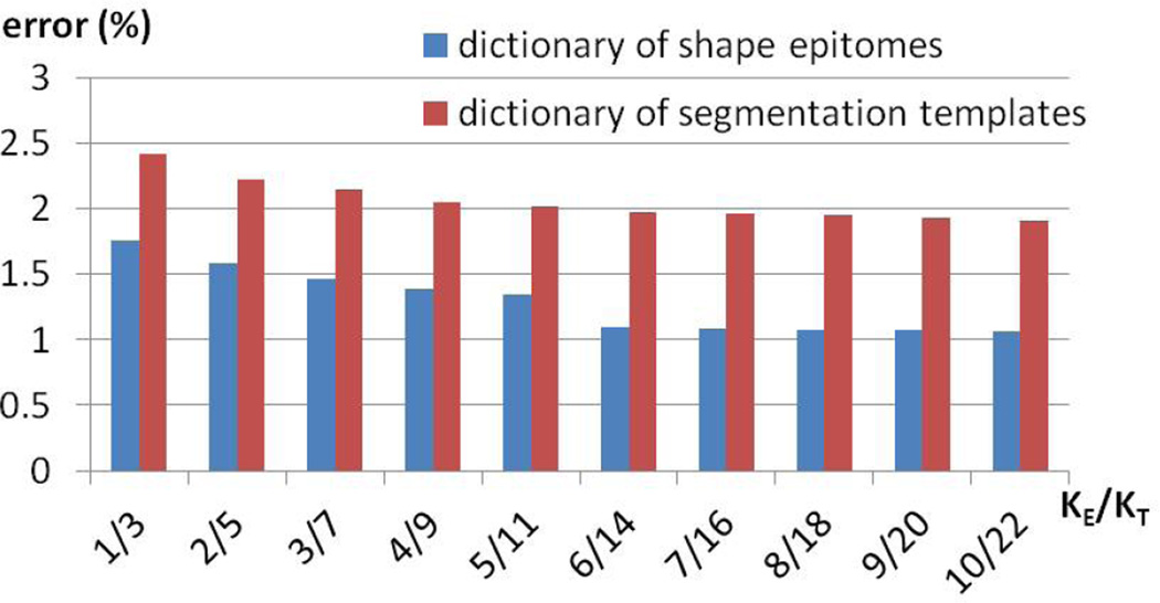
Here, we show the advantage of using our learned dictionary of shape epitomes over directly learning a dictionary of segmentation templates (in the latter case, the training shape patches have size m × m instead of M × M) by conducting experiments on the Stanford Background dataset, which provides more detailed object boundaries. We propose to compare those two dictionaries in terms of the error of encoding the ground truth, when given the same covered areas, which is equivalent to learning the same number of parameters. Suppose the size of the dictionary of shape epitomes is K_E, and the size of the dictionary of segmentation templates is K_T. Given K_E, to cover the same areas, we select K_T = 25²/17²K_E. As shown in Fig. 5, our learned dictionary of shape epitomes attains better performance than the dictionary of segmentation templates when given the same number of parameters.

Figure 5.

Error (%) of encoding ground truth of Stanford Background dataset, when using a dictionary of K_E shape epitomes or a dictionary of K_T segmentation templates.

4.3.2. Image labeling: MSRC-21 dataset

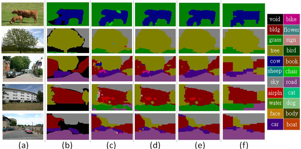
We generate 9 segmentation templates from each of the 5 shape epitomes in the labeling experiments (i.e., 181 templates totally). In a first set of experiments we directly compare our models with HIM [27]. We use the same boosting-based data term as HIM, provided by the authors, the main difference between HIM and our model lying in the representation part. As shown in Fig.7, our learned dictionary encodes the object shapes better than the hand-crafted dictionary used by HIM. Furthermore, both our Model 2 and Model 3 attain better performance than HIM (see Table 3).

Figure 7.

Qualitative results for the MSRC dataset. (a) Original image. (b) Ground truth. (c) Model 1. (d) Model 2. (e) Model 3. (f) HIM (excerpted from [27]). Note that our models capture object shapes more accurately than the HIM.

Table 3.

MSRC labeling results. Pixel-wise classification rates are provided for each category. Global accuracy refers to the pixel-wise classification rate averaged over the whole dataset, and Average accuracy refers to the mean of all object class classification rates. The Pxl-Cls model is the pixel-wise classifier, whose output is integrated in our models.

		building	grass	tree	cow	sheep	sky	airplane	water	face	car	bicycle	flower	sign	bird	book	chair	road	cat	dog	body	boat	Average	Global
Exp1 use same data term as HIM	Pxl-Cls	59.4	95.8	85.2	73.8	74.4	91.6	80.3	66.3	82.9	63.3	84.5	59.3	49.7	40.4	82.4	65.3	73.8	61.3	37.8	65.5	17.6	67.2	75.9
	Model 1	62.7	96.2	87.9	78.7	78.6	92.6	83.7	66.8	85.5	69.2	87.1	63.9	53.6	45.3	85.7	71.8	75.4	66.5	41.9	68.4	17.5	70.4	78.1
	Model 2	66.2	97.7	88.9	88.0	85.7	91.9	82.8	72.6	85.7	80.1	89.8	66.6	64.0	54.1	90.4	74.1	78.9	60.3	53.8	71.3	15.3	74.2	81.4
	Model 3	69.1	97.7	88.5	86.5	84.0	91.6	82.7	70.7	85.6	80.4	90.3	68.5	62.5	67.6	90.7	73.0	79.0	73.3	50.9	69.8	13.1	75.0	81.7
	HIM [27]	66.5	96.2	87.9	82.3	83.3	91.4	80.7	65.7	89.0	79.0	91.9	78.5	69.9	44.5	92.6	80.3	78.2	77.6	41.2	71.9	13.1	74.1	81.2
Exp2 use data term from Darwin software library	Pxl-Cls	55.9	95.9	82.0	77.1	71.1	90.3	72.4	69.1	79.7	54.3	78.7	62.2	42.5	38.8	64.3	58.0	84.4	59.4	39.8	64.4	27.8	65.2	74.5
	Model 1	63.9	96.9	86.6	81.9	75.2	91.9	76.1	72.8	81.3	59.9	84.4	65.8	45.5	41.7	66.1	61.9	87.7	64.0	43.4	67.5	29.4	68.7	77.6
	Model 2	71.6	98.3	91.9	90.1	76.1	94.5	68.3	78.3	82.2	57.3	84.7	74.0	44.7	35.8	73.6	55.4	88.7	67.0	44.9	61.8	23.6	69.7	80.4
	Model 3	73.0	98.1	92.3	91.4	78.4	94.4	70.6	77.2	82.5	60.2	86.2	73.4	48.4	35.3	76.8	60.3	89.0	68.0	44.6	63.1	22.2	70.7	81.1
	[9]	-	-	-	-	-	-	-	-	-	-	-	-	-	-	-	-	-	-	-	-	-	71.1	81.0
some state-of-the-art models	[19]	80	96	86	74	87	99	74	87	86	87	82	97	95	30	86	31	95	51	69	66	9	75	86
	[23]	63	93	88	84	65	89	69	78	74	81	84	80	51	55	84	80	69	47	59	71	24	71	78
	[8]	60	78	77	91	68	88	87	76	73	77	93	97	73	57	95	81	76	81	46	56	46	75	77
	DPG [22]	65	87	87	84	75	93	94	78	83	72	93	86	70	50	93	80	86	78	28	58	27	76	80
	[17]	-	-	-	-	-	-	-	-	-	-	-	-	-	-	-	-	-	-	-	-	-	78.3	86.0

We also compare our model with the recent method of [9] which incorporates powerful non-local patch similarity. We have used the same boosting-based data term as [9], as implemented in the Darwin software library¹. As shown in Table 3, our Model 3 attains similar performance to [9], although we do not use non-local cues at the patch level.

4.3.3. Image labeling: Stanford background dataset

In this experiment, we use the data term provided by the Darwin software library. The results for the Stanford Background dataset are shown in Fig. 8. We achieve comparable results with other state-of-the-art models. Specifically, our segmentation template-based Model 3 performs better than the more complicated model of [10], which builds on a dynamic superpixel representation and incorporates both semantic and geometric constraints in a slow iterative inference procedure. We also perform better than the hierarchical semantic region labeling method of [23]. Our models perform somewhat worse than the long-range model of [9] (unlike the MSRC case), and the segmentation tree model of [21], which however employs different image features.

Figure 8.

Qualitative and quantitative results on the Stanford Background dataset.

4.3.4. Scaling the segmentation templates

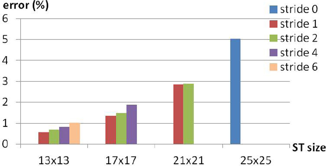
Here, we show that our learned dictionary can generate different sizes of segmentation templates, while attaining good performance on the Stanford Background dataset. Specifically, we explore the effect of varying the size of generated segmentation templates as the dictionary of shape epitomes is fixed. First, we explore the effect by encoding the ground truth. The size varies from m = {13, 17, 21, 25}. The stride variable is also changed to generate different number of segmentation templates from the dictionary. As shown in Fig. 6, the error is consistently decreased when m or stride is smaller. Second, we extract spatially equally 9 segmentation templates from the dictionary for different m (all resulting in 181 templates), and apply our Model 1 based on these templates to label the test images, as shown in Table 2. These results show that our proposed representation: shape epitomes is also able to handle scale effects without relearning the dictionary.

Figure 6.

Error (%) of encoding ground truth of Stanford Background dataset. The dictionary of shape epitomes is fixed. The size of generated templates is different, and so is the stride.

Table 2.

Reuse the dictionary of shape epitomes with different size of generated templates on Stanford Background dataset.

Template size	13 × 13	17 × 17	21 × 21
Global	76.9	76.7	76.3

5. Conclusion

In this paper, we introduced shape epitomes and showed that they could efficiently encode the edge structures in the MSRC and Stanford Background datasets. This efficient encoding is due to their ability to represent local shifts and rotations explicitly. The dictionary of shape epitomes were learnt from BSDS500 dataset. Next we explored the use of shape epitomes for CRF models of image labeling. The proposed SeCRF model can attain comparable results with other state-of-the-art models. Our supplementary material shows other applications of shape epitomes to edge detection and local appearance modeling.

References

- 1.Arbelaez P, Maire M, Fowlkes C, Malik J. Contour detection and hierarchical image segmentation. PAMI. 2011 doi: 10.1109/TPAMI.2010.161. [DOI] [PubMed] [Google Scholar]
- 2.Chatfield K, Lempitsky V, Vedaldi A, Zisserman A. The devil is in the details: an evaluation of recent feature encoding methods. BMVC. 2011 [Google Scholar]
- 3.Collins M. Discriminative training methods for hidden markov models: Theory and experiments with perceptron algorithms. ACL. 2002 [Google Scholar]
- 4.Delong A, Osokin A, Isack HN, Boykov Y. Fast approximate energy minimization with label costs. International Journal of Computer Vision. 2012 [Google Scholar]
- 5.Frey B, Dueck D. Clustering by passing messages between data points. Science. 2007 doi: 10.1126/science.1136800. [DOI] [PubMed] [Google Scholar]
- 6.Fulkerson B, Vedaldi A, Soatto S. Class segmentation and object localization with superpixel neighborhoods. ICCV. 2009 [Google Scholar]
- 7.Galleguillos C, Rabinovich A, Belongie S. Object categorization using co-occurrence, location and appearance. CVPR. 2008 [Google Scholar]
- 8.Gonfaus J, Boix X, Van De Weijer J, Bagdanov A, Serrat J, Gonzalez J. Harmony potentials for joint classification and segmentation. CVPR. 2010 [Google Scholar]
- 9.Gould S. Multiclass pixel labeling with non-local matching constraints. CVPR. 2012 [Google Scholar]
- 10.Gould S, Fulton R, Koller D. Decomposing a scene into geometric and semantically consistent regions. ICCV. 2009 [Google Scholar]
- 11.He X, Zemel R, Ray D. Learning and incorporating top-down cues in image segmentation. ECCV. 2006 [Google Scholar]
- 12.Jojic N, Frey B, Kannan A. Epitomic analysis of appearance and shape. ICCV. 2003 [Google Scholar]
- 13.Jurie F, Triggs B. Creating efficient codebooks for visual recognition. ICCV. 2005 [Google Scholar]
- 14.Kohli P, Ladicky L, Torr P. Robust higher order potentials for enforcing label consistency. IJCV. 2009 [Google Scholar]
- 15.Komodakis N, Paragios N. Beyond pairwise energies: Efficient optimization for higher-order mrfs. CVPR. 2009 [Google Scholar]
- 16.Kontschieder P, Buló S, Bischof H, Pelillo M. Structured class-labels in random forests for semantic image labelling. ICCV. 2011 doi: 10.1109/TPAMI.2014.2315814. [DOI] [PubMed] [Google Scholar]
- 17.Krähenbühl P, Koltun V. Efficient inference in fully connected CRFs with gaussian edge potentials. NIPS. 2011 [Google Scholar]
- 18.Kumar S, Hebert M. Discriminative random fields. IJCV. 2006 [Google Scholar]
- 19.Ladicky L, Russell C, Kohli P, Torr P. Associative hierarchical CRFs for object class image segmentation. ICCV. 2009 [Google Scholar]
- 20.Lafferty J, McCallum A, Pereira F. Conditional random fields: Probabilistic models for segmenting and labeling sequence data. ICML. 2001 [Google Scholar]
- 21.Lempitsky V, Vedaldi A, Zisserman A. A pylon model for semantic segmentation. NIPS. 2011 [Google Scholar]
- 22.Lucchi A, Li Y, Boix X, Smith K, Fua P. Are spatial and global constraints really necessary for segmentation? ICCV. 2011 [Google Scholar]
- 23.Munoz D, Bagnell J, Hebert M. Stacked hierarchical labeling. ECCV. 2010 [Google Scholar]
- 24.Roth S, Black M. Fields of experts. IJCV. 2009 [Google Scholar]
- 25.Shotton J, Johnson M, Cipolla R. Semantic texton forests for image categorization and segmentation. CVPR. 2008 [Google Scholar]
- 26.Shotton J, Winn J, Rother C, Criminisi A. Textonboost for image understanding: Multi-class object recognition and segmentation by jointly modeling texture, layout, and context. IJCV. 2009 [Google Scholar]
- 27.Zhu L, Chen Y, Lin Y, Lin C, Yuille A. Recursive segmentation and recognition templates for image parsing. PAMI. 2012 doi: 10.1109/TPAMI.2011.160. [DOI] [PubMed] [Google Scholar]
- 28.Zoran D, Weiss Y. From learning models of natural image patches to whole image restoration. ICCV. 2011 [Google Scholar]
Associated Data
This section collects any data citations, data availability statements, or supplementary materials included in this article.