Are older adults living in more equal counties healthier than older adults living in more unequal counties? A propensity score matching approach

Abstract

We assessed the potential contextual effect of income inequality on health by: 1) comparing individuals with similar socioeconomic status (SES) but who reside in counties with different levels of income inequality; and 2) examining whether the potential effect of county-level income inequality on health varies across SES groups. We used the Health and Retirement Study, a nationally representative study of Americans over the age of 50. Using propensity score matching, we selected SES-comparable individuals living in high-income inequality counties and in low-income inequality counties. We examined differences in self-rated overall health outcomes and in other specific physical/mental health outcomes between the two groups using logistic regression (n=34,994) and imposing different sample restrictions based on residential duration in the area. We then used logistic regression with interactions to assess whether, and if so how, health outcomes differed among participants of different SES groups defined by wealth, income, and education. In bivariate analyses of the unmatched full sample, adults living in high-income inequality counties have worse health outcomes for most health measures. After propensity score matching, adults in high-income inequality counties had worse self-rated health status (AOR=1.12; 95% CI 1.04–1.19) and were more likely to report diagnosed psychiatric problems (AOR=1.08; 95% CI 0.99–1.19) than their matched counterparts in low-income inequality counties. These associations were stronger with longer-term residents in the area. Adverse health outcomes associated with living in high-income inequality counties were significant particularly for individuals in the 30^th or greater percentiles of income/wealth distribution and those without a college education. In summary, after using more precise matching methods to compare individuals with similar characteristics and addressing measurement error by excluding more recently arrived county residents, adults living in high-income inequality counties had worse reported overall physical and mental health than adults living in low-income inequality counties.

I. Background

Compared to their peers in other high-income countries, Americans have worse health and higher mortality rates (Banks, Marmot, Oldfield, & Smith, 2006; Banks, Muriel, & Smith, 2010; Cohen, Preston, & Crimmins, 2011; Crimmins, Preston, & Cohen, 2011; J. Y. Ho, 2013; Jessica Y Ho & Preston, 2010; Woolf & Aron, 2013). Income inequality is also significantly greater, with the United States ranking as the fourth most unequal country among 34 high-income countries (OECD, 2013). Numerous ecological studies have shown a significant association between higher income inequality, measured at the national-, state-, or community- levels, and worse population health (Kaplan, Pamuk, Lynch, Cohen, & Balfour, 1996; Kennedy, Kawachi, & Prothrow-Stith, 1996). However, multilevel analyses have reached mixed conclusions about the contextual effects of income inequality on population health (Ash & Robinson, 2009; Babones, 2008; Ben-Shlomo, White, & Marmot, 1996; Daly, Duncan, Kaplan, & Lynch, 1998; Deaton & Lubotsky, 2003, 2009; Fiscella & Franks, 1997; Fisella & Franks, 2000; Kennedy, Kawachi, Glass, & Prothrow-Stith, 1998; LeClere & Soobader, 2000; Lochner, Pamuk, Makuc, Kennedy, & Kawachi, 2001; J. W. Lynch et al., 1998; Muramatsu, 2003; Soobader & LeClere, 1999; Wilkinson & Pickett, 2006, 2008). Systematic literature reviews and meta-analyses suggest that studies examining income inequality over larger geographic boundaries (e.g., states) are more likely to report significant associations between income inequality and health, compared to studies examining income inequality over smaller geographic units (e.g., county or census tract) (Kondo et al., 2009; S. V. Subramanian & Kawachi, 2004; Wilkinson & Pickett, 2006).

A number of studies have also found mixed results for the contextual effect of income inequality on health across socioeconomic groups. Lochner et al. (2001) found that the mortality risk of near-poor individuals was more strongly associated with state income inequality than the mortality risk of the poor (Lochner et al., 2001). Subramanian et al. (2001) reported a differential impact of state income inequality on high-income groups, such that the affluent report better health from living in high inequality states (S.V. Subramanian, Kawachi, & Kennedy, 2001). In contrast, according to Subramanian and Kawachi (2006), income inequality exerts a comparable contextual effect across all socioeconomic sub-groups with self-rated health status (S. V. Subramanian & Kawachi, 2006).

These studies examining the association between income inequality and health attempted to control for measured confounders by including individual-level socio-economic characteristics as independent variables in multiple regression analyses. A far more rigorous method to adjust for potential confounders, such as socioeconomic status (SES), would compare the health outcomes of a matched sub-sample of individuals with similar demographic and socioeconomic characteristics, but who live in places with different levels of income inequality. Yet, to our knowledge, no prior multilevel analyses to date have used a matched sample based on a propensity scores to select individuals who are comparable on their SES characteristics to assess the possible contextual effect of income inequality on adult health. Filho et al. (2012) used a propensity score matching technique to match districts but not individuals, using an aggregate, district-level dataset (Chiavegatto Filho, Kawachi, & Gotlieb, 2012). To assess individuals’ health differences attributable to the level of income inequality of the place where they reside, a better approach is to match study samples at the individual level, based on individuals’ demographic and socioeconomic attributes, and then examine differences in health outcomes between those who live in high versus low-income inequality places.

Another important empirical issue in identifying whether a contextual measure of income inequality is associated with health outcomes is the potential measurement error that could occur as a result of recent migration to the area, as recent arrivals may not have lived in the community long enough to experience any consequences of local conditions. To experience health consequences, individuals would likely need to be exposed to the local conditions for some time. However, to our knowledge, no prior study has addressed the potential measurement error resulting from the inclusion of individuals who have recently moved to the area.

Accordingly, in this study, we aimed to contribute to the literature by: 1) improving the measurement of a potential contextual effect of income inequality on residents’ health by using a propensity score matching technique to identify comparable individuals living in counties with different income inequality levels; 2) addressing the measurement error in the potential income inequality effect which arises from varying lengths of residence in the area; and 3) assessing whether any contextual effect on key health outcomes is moderated by individual/family-level socioeconomic status, as measured by educational attainment, household income, and household wealth.

II. Conceptual Model

Our conceptual model is based on existing theory and prior research linking levels of income inequality and individual health through both material and psychosocial pathways (Brunner & Marmot, 2005; Daly et al., 1998; Kondo et al., 2009; J. Lynch et al., 2004; S. V. Subramanian & Kawachi, 2006). Figure 1 shows the conceptual model guiding our hypotheses regarding the mechanisms by which area-level income inequality could influence individuals’ health outcomes, independent of individual-level demographic and socioeconomic status.

Figure 1.

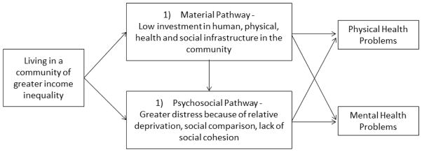
Potential Causal Pathways linking Community-level Income inequality and Individuals’ Health Outcomes

Material pathways suggests that living in a place of high-income inequality is associated with a set of economic, political, social, and institutional processes reflecting systematic underinvestment in human, physical, health, and social infrastructures (Daly et al., 1998). As a result, residents may have fewer resources to buy housing, healthy food, medical care and have access to a lower quality education, health services, transportation, recreational facilities, and/or publicly provided services. As a consequence, the physical and mental health of residents may suffer (J. Lynch et al., 2004).

In terms of psychosocial factors, inequitable income distribution may influence individuals’ perceptions of and experiences with their social environment in ways that undermine mental health (Daly et al., 1998). Important aspects of the perceived social environment include relative poverty, relative economic insecurity, and lack of social cohesion and trust. Feelings of relative deprivation may affect both the endocrine and immune systems (Brunner & Marmot, 2005). Therefore, individuals living in a place of high-income inequality may have greater distress, and hence have poor health. Moreover, psychosocial factors such as fear of losing one’s current socioeconomic status in the face of weak safety nets and lack of trust and cohesion that come with greater income inequality may affect the health of not just the poor, but even higher SES individuals that live there as well (Kondo et al., 2009; S. V. Subramanian & Kawachi, 2006).

The conceptual model also suggests the magnitude of the potential contextual effect of income inequality on health may well vary depending on individuals’ SES. Each of these material and psychosocial pathways might have different effects depending on the social and economic circumstances of individuals. More specifically, material pathways are likely to affect the health of both poor and middle-class individuals (Daly et al., 1998) but not necessarily the health of high-income individuals. Although the psychosocial pathways may affect all SES groups, because the health of low income individuals is affected by their own poor economic circumstances to a large extent, additional health effects of living in a higher income inequality area may not translate into an increased risk of health problems for these low income individuals. While there is extensive research on health differences among individuals by area-level income inequality, and separately by individuals’ SES, few studies have discussed whether and if so, how, the potential contextual effect of income inequality might interact with individuals’ social and economic status.

III. Specific Research Questions and Hypotheses

In this paper, we sought to assess the contextual effect of income inequality on health using more rigorous methods than have been used in prior studies to control for individual-level characteristics. We then look for variation in the association between income inequality and health by individuals’ education and economic status. More specifically, our research questions and hypotheses are:

1. Do adults living in a high-income inequality county have worse health outcomes than adults living in a low-income inequality county, even when comparing adults with similar demographic and socioeconomic characteristics? Based on the conceptual model above, we hypothesized that we would find worse self-rated overall health and mental health among individuals living in high-income inequality counties, even after matching individuals on demographic and socioeconomic characteristics. We also hypothesized that the health differences between two income–inequality county groups would be greater if we restrict the analysis to individuals who have lived in the area for a longer period of time.

2. Which socioeconomic groups are more susceptible to the health effects of county-level income inequality? We hypothesized that the association between county-level income inequality and health is more pronounced among individuals with low to middle SES because the material pathways would be especially salient in these groups. The psychosocial pathways, such as distress from lack of social cohesion and trust, may affect all SES groups, but we hypothesized that the health effects of these non-material pathways may not be substantial enough to significantly affect physical health for the very high socioeconomic group. At the same time, the health of lower SES groups is likely to be significantly poorer compared to that of higher SES groups independent of the county level of income inequality. Therefore, it is uncertain to what extent marginal increases in health problems attributable to income inequality of the area will be statistically and clinically significant.

IV. Data and Sample

We used the Health and Retirement Study (HRS), a biannual, longitudinal study that since 1998 is nationally representative of U.S. adults over the age of 50 (http://hrsonline.isr.umich.edu/). Because the HRS has a sample of approximately 20,000 adults who are surveyed every two years on a comprehensive set of health, demographic, and socioeconomic indicators, we were able to obtain a sizable analytic sample after propensity score matching at the individual level. To obtain a county-level income inequality measure (measured by a Gini-index), we used the American Community Survey (ACS), an ongoing monthly survey by the U.S. Census Bureau. The ACS was fully implemented in 2005 and is the largest household survey in the United States, with a sample size of about 3 million housing unit addresses through the country (Webster, 2010). To obtain comparable income inequality measures prior to 2005, we used the 2000 U.S. decennial census to obtain the 2000 Gini-index and interpolated values for 2002 and the 2004 Gini-indices based on the 2000 U.S. decennial census and 2005–2007 waves of ACS. At the time of writing of this manuscript, detailed geographic information for each respondent in the HRS was available only up to the 2010 survey year. Accordingly, we examined county-level income inequality measures and contemporaneous health outcome measures of the HRS sample of adults from 2000–2010.

To employ the propensity-score matching method, we categorized respondents into three groups based on the distribution of their county’s Gini-index in a given year (low, medium, and high-income inequality). We then selected the low-income inequality (bottom 33%) group of individuals and the high-income inequality group (top 33%), dropping the middle group from our analyses in order to select matched sub-samples from distinct income inequality groups. We then defined two analytic samples: 1) the non-matched sample of all HRS respondents who lived in the lowest and highest income inequality counties, and 2) the propensity score matched (PSM) sample, a sub-sample including only matched respondents from counties of high or low-income inequality. The PSM sample is our primary analytic sample, and all analyses utilize the dataset as a pooled, multilevel cross-sectional dataset, such that respondents can contribute up to six respondent-year observations. The non-matched sample from low- and high-income inequality counties contains 70,773 respondent-year observations. In the PSM sample, there are 34,994 such respondent-year observations. There are missing values in some individual/family-level covariates and health outcomes ranging from 0.02% (e.g., race) to 8% (e.g., CESD). Therefore, number of observations used for estimation will vary depending on estimation models. We used imputation for missing values in one of the sensitivity analyses described below.

V. Measures

Health Outcomes

We examined measures of physical health and mental health. We used self-rated health (SRH) status as our primary health measure because SRH is a well-validated global health measure of both physical health and mental health and is the most widely used outcome in the study of income inequality and individual health (Idler & Benyamini, 1997; Kondo et al., 2009; Lee, 2000). It has five response categories (excellent, very good, good, fair, poor). We created a dichotomous measure indicative of fair/poor health status for the analyses as was done in most prior studies (Kondo et al., 2009). Other health indicators included two validated measures of disability status: limitations in activities of daily living (ADLs) and instrumental activities of daily living (IADLs) (Sandy Chien, August 2013). The ADL index measures difficulty in six daily activities: walking across a room, dressing, bathing, eating, getting in/out of bed, and toileting. The IADL index measures difficulty in five instrumental activities: using a telephone, taking medication, handling money, shopping, and preparing meals. We created a dichotomized indicator of having difficulty in at least one ADL and a dichotomized indicator of having difficulty in at least one IADL. We also examined whether participants reported that a doctor had ever told them that they had high blood pressure, heart disease, a stroke, or diabetes. We examined two measures of mental health: the Center for Epidemiologic Studies Depression (CESD) scale which measures depressive symptoms based on six negative and two positive (reverse coded for the scale) items (Sandy Chien, August 2013); and a measure of whether the participant reported having been diagnosed with a psychiatric problem. We used an indicator of four or more depressive symptoms, a cut-off used for clinically significant depression in the literature (Mezuk, Bohnert, Ratliff, & Zivin, 2011; Steffick, 2000). Diagnoses of each disease (high blood pressure, heart disease, stroke, diabetes, and psychiatric problem) were used as dichotomous indicators (yes or no).

Income inequality

The county-level Gini-index in a given year was used as our income inequality measure. To employ the propensity-score matching method, we categorized respondents into three groups based on the distribution of county-level Gini-indices in a given year (low, medium, and high-income inequality). For example, in 2010, the range of Gini-index is 0.332 to 0.437 (standard deviation=0.017) in the bottom 33%, 0.438 to 0.470 (standard deviation=0.009) in the middle 33%, and 0.471 to 0.600 (standard deviation=0.020) in the top 33%. We then selected the low-income inequality group (bottom 33%) and the high-income inequality group (top 33%) and created an indicator of high-income inequality for the analyses (1 if the individual lives in top 33% Gini-index county, 0 if individuals live in the bottom 33% Gini-index county).

Years of living in/around the current main residence

The HRS asked all respondents how many years they had lived in/around their main residence in 1995 and 1996. In subsequent survey waves, the HRS asked the question to existing respondents only if they had changed their main residence since the prior interview or if the respondents were newly added to the survey wave. By tracking respondents’ residential histories for 1995–2010, we constructed a measure of the number of years each respondent had lived in/around the area for each survey wave during the study period (2000–2010). For example, if a respondent reported he had lived in/around in his residence for ten years for the 1996 interview, and that respondent reported during 2004 interview that he changed his residence since the last interview and moved into his current home in 2003 but no further changes in residence were reported for 2006–2010 interview years, the number of years living in/around the current main residence for that respondent was coded as 14 years in 2000, 16 years in 2002, 1 year in 2004, 3 years in 2006, 5 years in 2008, and 7 years in 2010.

Individual/household-level Demographic and Socioeconomic Characteristics

To assess the potential contextual effect of income inequality on health outcomes, we matched our sample on individual-level characteristics that have been identified as important factors influencing individuals’ health and that are likely to be related to the income inequality level of their area of residence. We included age (<64, 65–74, >75), race (White indicator), and ethnicity (Hispanic indicator) as potential demographic variables that are associated with both individuals’ health and area-level income inequality. We matched on marital status (currently had a spouse) because a spouse is one of the most prevalent caregivers for older persons and hence likely to affect older persons’ health. Social class inequality in health has been discussed extensively in the literature, and education, wealth and income are among the most important predictors of health and mortality (Elo, 2009). Accordingly, we matched on the respondent’s education with five categories: no degree, GED/high school, at least some college. Quartile of total household wealth was used for matching and decile of wealth was used to examine potential variation in the contextual effect for respondents with different levels of household wealth. Total household income was also used in both forms (quartile and decile) as for total household wealth.

VI. Analytic Approach

Propensity score matching

Demographic and socioeconomic status of individuals may substantially differ between low-income inequality areas and high-income inequality areas. In general, where there is not sufficient overlap in covariates between the treatment and control groups, the high versus low income inequality areas, the resulting treatment effect estimates would rely heavily on extrapolation in traditional regression models. Therefore, we employed a propensity score matching method for our primary analyses to balance covariates of individual-level demographic and socioeconomic characteristics of residents between low- and high- income inequality areas. We first identified respondents who live in the selected low or high-income inequality counties (defined above) at a given year. We then calculated the propensity score using logistic regression with an indicator of high-income inequality as the dichotomous outcome and a broad set of predictors of observed individual-level covariates (age, gender, race/ethnicity, marital status, education, wealth, income, and years of living in/around current residence). Finally, we matched individuals between two income inequality groups (low and high) based on the propensity score at a given year. Using a Stata command psmatch2 (version 4.0.5), we implemented one-to-one nearest neighbor matching within a caliper (Guo & Fraser, 2014; Leuven & Sianesi, 2014; Sianesi, 2010) at a given year. Therefore, each respondent was matched to only one other respondent in a given year. Our matching goal was to balance the sample over all covariates between high- and low- income inequality groups. We determined caliper size accordingly. More specifically, we started with a caliper size of a quarter of a standard deviation of the estimated propensity scores, typically suggested as the maximum caliper size (Guo & Fraser, 2014). We then lowered the caliper size until the resulting matching achieved a complete balance (i.e., no significant difference in any covariate between the two groups). After this process, our final caliper value was set at 0.0001.

Estimation of the association between area-level income inequality and health outcomes

Using the propensity-score matched (PSM) sample, we assessed potential differences in health outcomes between individuals who lived in a county of low-income inequality and those who lived in a county of high-income inequality. We controlled for time trend by including year indicators for 2002–2010. More formally, by denoting a person i’s health outcome in year t as H_i,t, an indicator of a person i’s living in a high-income inequality county in year t as $I_{i,t}^{\mathit{high}}$ (=1 if high-income inequality; 0 if low-income inequality), and an indicator of year t as D_t, we can specify our baseline model as:

$$H_{i,t}={\beta }_0+{\beta }_1{I}_{i,t}^{\mathit{high}}+{\beta }_2^t\sum _{t=2002}^{t=2010}{D}_t+{\epsilon }_{it}$$

We estimated odds ratios of poor health between two income inequality groups using logistic regression models. We then examined whether the estimated associations change when the sample is restricted by the number of years a respondent resided in the area (>=5 years; >=15 years; >=30 years).

In secondary analyses, we also examined traditional bivariate and multivariate analyses using the non-matched sample, which includes all respondent-year observations from low and high-income inequality groups.

SES variations in the association between area-level income inequality and health outcomes

Using the PSM sample, we examined variations in the contextual income inequality effect depending on respondents’ SES (household wealth decile, household income decile, and highest degree/diploma). The estimation model includes an interaction term between the income inequality indicator and a SES measure as well as the level of income inequality indicator and the SES measure, demographic characteristics, and year indicators. Accordingly, we can specify the model as:

$$H_{i,t}={\beta }_0+{\beta }_1{I}_{i,t}^{\mathit{high}}\times {\mathit{SES}}_{i,t}+{\beta }_2{I}_{i,t}^{\mathit{high}}+{\beta }_3{\mathit{SES}}_{i,t}+{\beta }_4{\mathit{Demo}}_{i,t}+{\beta }_5^t\sum _{t=2002}^{t=2010}{D}_t+{\epsilon }_{it}$$

We conducted multivariate logistic regression for estimation and then obtained marginal effects of high-income inequality (i.e., difference in predicted probability of poor/fair SRH between high and low-income inequality groups) at specific levels of each SES measure (wealth, income, education), after holding demographic covariates at each respondent’s own values (Williams, 2012). Each SES measure was examined separately (i.e., we did not include multiple SES measures in one multivariate logistic regression).

Imputation

In sensitivity analyses, we repeated our analyses with one fully imputed dataset. We employed chained equations, a sequence of univariate imputation methods with fully conditional specification (FCS) of the prediction equation (Raghunathan, Lepkowski, Van Hoewyk, & Solenberger, 2001; Royston, 2009; White, Royston, & Wood, 2011), stratified by year. We imputed all measures used in the analyses (demographic, SES, Gini-index of county, and health).

Because respondents and their spouse can contribute to analyses as multiple observations over the sample period (2000–2010), we clustered residual structure at the family level to obtain robust standard errors in all analyses (Rogers, 1994). All analyses are conducted using Stata 13.

VII. Results

Table 1 shows summary statistics of the demographic characteristics, socioeconomic status, and residential duration (i.e., years of living in/around the current residence) of respondents in high and low-income counties. In the non-matched sample of respondent-year observations, there are significant differences in the demographic and socioeconomic characteristics (except for age) between respondents living in low-income inequality counties and in high-income inequality counties. Compared to those living in the low-income inequality counties, those from high-income inequality counties are more likely to be women, non-white, Hispanic, unmarried, less-educated, and have lower wealth, lower household total income, and longer residence in the area. In the PSM sample that contains only respondents matched over variables listed in Table 1, there are no significant differences in demographic characteristics or socioeconomic status across the high versus low-income inequality groups. This validates the PSM sample for our primary analyses.

Table 1.

Summary Statistics of Sample: Individual Characteristics before and after Matching

	Non-matched Sample			Propensity Score Matched (PSM) Sample
	(1) Low Income Inequality (N=34,300)	(2) High Income Inequality (N=36,473)	p-value	(3) Low Income Inequality (N=17,504)	(4) High Income Inequality (N=17,504)	p-value
	proportion	proportion		Proportion	Proportion
Women	0.57	0.59	<0.001	0.59	0.58	0.200
Age			0.567			0.229
51–64	0.40	0.42		0.38	0.38
65–74	0.32	0.32		0.33	0.33
>75	0.28	0.27		0.30	0.29
White	0.91	0.68	<0.001	0.88	0.88	0.961
Hispanic	0.04	0.16	<0.001	0.05	0.05	0.981
With spouse/partner	0.67	0.59	<0.001	0.66	0.66	0.392
Education			<0.001			0.680
Less than high school	0.19	0.30		0.20	0.20
High school/GED	0.56	0.47		0.55	0.55
At least some College	0.17	0.15		0.17	0.17
Advanced Degree	0.08	0.09		0.08	0.09
Total Household Wealth			<0.001			0.330
Bottom 25%	0.19	0.32		0.22	0.21
25–50%	0.25	0.26		0.24	0.24
50–75%	0.28	0.21		0.26	0.26
Top 25%	0.28	0.21		0.29	0.29
Total Household Income			<0.001			0.345
Bottom 25%	0.20	0.32		0.22	0.22
25–50%	0.25	0.24		0.24	0.25
50–75%	0.28	0.22		0.26	0.26
Top 25%	0.28	0.22		0.28	0.28
Years of living in/around current residence			<0.001			0.775
<=10	0.34	0.27		0.31	0.30
>10&<=30	0.24	0.23		0.24	0.24
>30	0.42	0.49		0.46	0.46

Association between County-level Income inequality and Health before Propensity Score Matching

Table 2 presents odds ratios for each health outcome in the logistic regression models and the predicted probabilities of worse health outcomes in each group by level of income inequality, using the non-matched sample. In the bivariate analyses in the top panel, the health of those who live in high-income inequality counties is worse on all health measures except for prevalence of stroke. The percentage of respondents reporting fair/poor SRH is 9.0 percentage points greater in the high-income inequality counties (34.9% versus 25.9%), yielding a bivariate odds ratio of 1.53 (95% CI 1.45–1.61). After adjusting for demographic and socioeconomic characteristics and years of living in the area in multivariate logistic regressions (see bottom panel of Table 2), only the association between county-level income inequality and self-rated health (SRH) remained statistically significant and was smaller in magnitude (AOR=1.15; 95% CI 1.08–1.21).

Table 2.

Odds Ratios of Health Outcomes for High-income inequality: Before Propensity Score Matching

	Primary Outcome	Secondary Outcomes
	(1) Fair/poor SRHS	(2) At least one limitation in ADL	(3) At least one limitation in IADL	(4) 4 or greater CESD	(5) High Blood Pressure	(6) Diabetes	(7) Heart disease	(8) Stroke	(9) Psychiatric problem
I. Non-matched Sample: Bivariate (OR, 95%CI)	(N=70719) )	(N=70773) )	(N=70655) )	(N=64683) )	(N=70667) )	(N= 70712) )	(N=70704) )	(N=70732) )	(N=70689) )
	1.53*** (1.45,1.61)	1.28*** (1.21,1.35)	1.30*** (1.22,1.38)	1.37*** (1.28,1.45)	1.15*** (1.09,1.22)	1.23*** (1.15,1.32)	0.91** (0.85,0.96)	1.07 (0.97,1.19)	1.07* (1.00,1.15)
Percent in
low income-inequality (Bottom 33% of Gini-index)	25.9%	20.4%	14.6%	13.5%	55.2%	18.5%	25.7%	7.0%	16.0%
high income-inequality (Top 33% of Gini-index)	34.9%	24.6%	18.2%	17.6%	58.7%	21.9%	23.9%	7.5%	17.0%
II. Non-matched Sample: Multivariate (OR, 95%CI)	(N=66249) )	(N=66297) )	(N=66184) )	(N=60733) )	(N=66200) )	(N=66241) )	(N=66232) )	(N=66259) )	(N=66222) )
	1.15*** (1.08,1.21)	1.01 (0.95,1.08)	1.04 (0.97,1.11)	1.04 (0.97,1.11)	0.98 (0.92,1.04)	0.97 (0.89,1.04)	0.97 (0.90,1.04)	0.94 (0.84,1.05)	1.03 (0.95,1.12)
Predicted Probability in
low income-inequality (Bottom 33% of Gini-index)	29.4%	22.9%	16.6%	15.5%	57.8%	20.6%	25.6%	7.6%	16.4%
high income-inequality (Top 33% of Gini-index)	31.9%	23.2%	17.1%	15.9%	57.2%	20.1%	25.0%	7.2%	16.8%

^*p<0.05,

^**p<0.01,

^***p<0.001

Association between County-level Income inequality and Health after Propensity Score Matching

Table 3 shows results in the propensity score matched sample, without and with sample restrictions on the number of years resident in the area. In these results for the full PSM sample, living in a high-income inequality county is associated with significantly poorer SRH (AOR=1.12; 95% CI 1.04–1.19) and a greater risk of having a psychiatric diagnosis (AOR=1.08; 95% CI 0.99–1.19). There were no significant associations between living in a high-income inequality county and other health measures.

Table 3.

Odds Ratios of Health Outcomes for High-income inequality: After Propensity Score Matching

	Primary Outcome	Secondary Outcomes
	(1) Fair/poor SRHS	(2) At least one limitation in ADL	(3) At least one limitation in IADL	(4) 4 or greater CESD	(5) High Blood Pressure	(6) Diabetes	(7) Heart disease	(8) Stroke	(9) Psychiatric problem
>= 0 years (OR, 95%ci)	(N=34983)	(N=35008)	(N=34952)	(N=32688)	(N=34982)	(N=34990)	(N=34987)	(N=34994)	(N=34986)
	1.12** (1.04,1.19)	1.01 (0.94,1.09)	1.04 (0.96,1.13)	1.05 (0.97,1.14)	0.98 (0.91,1.04)	0.97 (0.89,1.06)	0.97 (0.90,1.05)	0.98 (0.86,1.11)	1.08+ (0.99,1.19)
>=5 years (OR, 95%CI)	(N=28651)	(N=28670)	(N=28626)	(N=26749)	(N=28651)	(N=28654)	(N=28652)	(N=28659)	(N=28648)
	1.13*** (1.06,1.22)	1.03 (0.95,1.12)	1.12* (1.03,1.23)	1.06 (0.97,1.16)	0.98 (0.91,1.05)	0.99 (0.90,1.08)	1.01 (0.93,1.10)	1.03 (0.89,1.19)	1.12* (1.01,1.24)
>=15 years (OR, 95%CI)	(N=22339)	(N=22354)	(N=22324)	(N= 20789)	(N=22337)	(N=22340)	(N=22338)	(N=22345)	(N= 22338)
	1.17*** (1.08,1.27)	1.03 (0.94,1.13)	1.13* (1.02,1.25)	1.09 (0.98,1.21)	0.98 (0.90,1.06)	0.96 (0.86,1.07)	1.04 (0.94,1.14)	1.00 (0.85,1.17)	1.16* (1.03,1.31)
>=30 years (OR, 95%CI)	(N=16439)	(N=16451)	(N= 16435)	(N=15199)	(N= 16440)	(N=16443)	(N=16441)	(N= 16447)	(N=16438)
	1.17** (1.06,1.28)	1.06 (0.95,1.18)	1.14* (1.01,1.28)	1.06 (0.94,1.20)	1.00 (0.90,1.10)	0.95 (0.83,1.07)	1.03 (0.92,1.15)	1.00 (0.83,1.20)	1.14+ (0.99,1.31)

⁺<0.1,

^*p<0.05,

^**p<0.01,

^***p<0.001

The positive association between income inequality and poor/fair SRH tends to increase as we restrict the analytic sample to individuals with longer residence (from AOR=1.12 for zero or greater years of residence to AOR=1.17 for 15 years or longer, p=0.05). A similarly increasing pattern in the association with longer residence is also found in the risk of psychiatric diagnosis (from AOR=1.08 with zero or greater years of residence to AOR=1.16 with 15 years or longer, p=0.04).

Variations in the Association between Health and Income inequality by Household’s Wealth and Income and Individual’s Education

Figures 2, 3, and 4 present results of multivariable logistic regressions including interactions between high-income inequality county and individual-level SES characteristics. We focused on outcomes of self-rated health (SRH) and diagnosis of psychiatric problem because these two outcomes were significantly related with county-level income inequality in the PSM sample. The potential adverse effect of income inequality on SRH was likely to be observed at 30th or greater percentiles in the distribution of household wealth and total income (Figure 2 & Figure 3). For example, living in a high-income inequality county increased the predicted probability of an adult in the 50^th percentile wealth group reporting poorer SRH by about 0.03 (95% CI 0.012 – 0.040), compared to the predicted probability of that adult living in a low-income inequality county (0.31 versus 0.28, respectively). The potential adverse effect of living in a high-income inequality county on poorer SRH is also likely to be found for adults who had no college education but not for those with more education (Figure 4). For example, the potential risk of poorer SRHS increased by 0.04 (95% CI 0.005–0.067) for an adult with no degree who lived in a high-income inequality county instead of low-income inequality county (0.46 versus 0.42, respectively). No specific economic (wealth/total income) subgroup in our analyses was identified to have a significant relationship between income inequality of county and diagnosis of psychiatric problem at the significance level of 5% p-value, but have a significant relationship at the significance level of 10% p-value for the 40^th and 50^th percentiles. The potential effect of high-income inequality on the diagnosis of psychiatric problem is significant for adults who have high school/GED only (marginal effect: 0.02; 95% CI 0.002–0.03), but not for other education groups (results available on request).

Figure 2. Variations over Household Wealth in Marginal Effect of High-income inequality (Propensity Score Matching Sample).

Note: Marginal effects and 95% confidence intervals for the high-income inequality group are shown for each decile of household wealth, using the propensity score matched sample. A positive value indicates greater risk of fair/poor SRH for high-income inequality group, compared to that for the low-income inequality group, at a given household wealth decile.

Figure 3. Variations over Household Total Income in Marginal Effect of High-income inequality (Propensity Score Matching Sample).

Note: Marginal effects and 95% confidence intervals for the high-income inequality group are shown for each decile of household total income, using the propensity score matched sample. A positive value indicates greater risk of fair/poor SRH for high-income inequality group, compared to that for the low-income inequality group, at a given household total income decile.

Figure 4. Variations by Degrees/Diploma in Marginal Effect of High-income inequality (Propensity Score Matching Sample).

Note: Marginal effects and 95% confidence intervals for the high-income inequality group were shown for each education level, using the propensity score matched sample. A positive value indicates greater risk of fair/poor SRH for high-income inequality group, compared that for the low-income inequality group, at a given education level.

Results from the Imputed Dataset

After imputation, the propensity score sample included 40,574 respondent-year observations. Primary results for SRH are consistent with those from the dataset without imputation (e.g., AOR=1.12 from both datasets, with and without imputation). However, when using the imputed dataset, the health difference in psychiatric diagnosis was not statistically significant using the full sample, but significant in more restricted sample for longer-term residents (years of residential duration >=5). A result table from the imputed dataset was not included in the manuscript.

VIII. Summary and Discussion

In this national sample of US adults over 50, adults living in high-income inequality counties are more likely to report fair or poor self-rated health when compared to those living in low-income inequality counties. The use of propensity score matching decreased substantially the health gap between residents in high-income inequality counties and those in low-income inequality counties, compared to that from the non-matched sample. However, the gap in self-rated health remained statistically significant in the propensity score matched sample. This suggests that while individual-level demographic characteristics and socioeconomic status explain a large part of health gap between those living in low versus high-income inequality counties, living in a high-income inequality area itself might be an independent risk factor for less favorable self-rated health assessments by residents.

Respondents living in higher income inequality counties also reported worse functional status, more depressive symptoms, and were more likely to report having high blood pressure, diabetes, and a psychiatric diagnosis than those in low-income inequality counties according to results from non-matched sample. However, with the exception of having a psychiatric diagnosis, health gaps by county-level income inequality dissipated in the propensity score matched sample.

We hypothesized that the association between county level income inequality and individual residents’ health would be more likely to exist for low and middle-income individuals. This is consistent with our empirical finding of variation in the association by education; the potential contextual effect is most likely to be found among adults with no college degree. Our findings for variation in health gaps by wealth and income, however, suggest that the potential contextual effect of income inequality on SRH is most likely to be found among middle and high economic groups. The point estimates for low economic groups are not substantially different from middle/high economic groups, but there seem to be more heterogeneity among those in low economic groups, yielding non-significant findings. This result is not directly comparable with earlier literature on SES variations in the contextual effect of income inequality on health, because our population of interest and unit of geography are different from those relevant studies listed earlier.

Several limitations to our analyses should be noted. First, because our primary analysis is from a subsample of HRS to select only propensity-score matched observations, the analysis sample may not be as nationally representative as the original HRS sample from which it is drawn. Second, we created three income inequality groups – low (33%), medium (33%), and high (33%) - based on the Gini-index of the county,—but then only compared the low and high groups. We conducted a sensitivity analysis by using different cut-points to identify low and high inequality counties which did not change our findings. For example, results from comparing counties in the lowest 20% of the Gini-index and counties with in the highest 20% of the Gini-index, or using the lowest and highest 40%, were not substantively different from results presented above. It is not clear in the literature what level of income inequality affects health. More empirical investigations using different cut-points for income inequality groups is needed to identify threshold effects. Third, one might argue that by selecting individuals who have similar socioeconomic status, we tend to control for economic pathways through which contextual effects of income inequality might operate. For example, if part of the reason for residents having low economic status is attributable to living in a high-income inequality place, by comparing individuals with similar economic conditions, we might understate the potential health gap attributable to area-level income inequality. Fourth, our health outcome measures are self-reported. Future research should examine more objective measures such as biomarkers and medical record data.

Despite these limitations, our research contributes to current literature on contextual effect of income inequality on health in several key ways. First, using propensity score matching, we were able to balance sample composition between two comparison groups – those living in high and low-income inequality counties. To our knowledge, this is the first multilevel study that examined subsamples of matched individuals to assess the contextual effect of income inequality on residents’ health. Second, we constructed each respondent’s residential history after carefully examining information on residential migration by utilizing the longitudinal structure of the HRS, and then incorporated residential duration into the analysis. Because we are focusing on the contextual effect of living in a certain kind of area, it is essential to balance the duration of residents’ exposure to their current environment between the two income inequality groups. Suppose adults tend to move to a more equal (or more unequal) area because of health problems associated with aging. Ignoring adults’ duration of residence would tend to understate (or overstate) the health gap for residents of low and high-income inequality places. Moreover, for the health of an individual to be affected by the area in which she lives, that individual probably should have resided there for at least some time. Despite the importance of these potential measurement issues associated with residential duration, to our knowledge, no previous study examining contextual effects of income inequality on adult health has addressed duration of residence. Finally, we assessed variation by individual respondents’ SES in the contextual association between income inequality and health outcomes, using multiple indicators of SES including education, income, and wealth. The question of heterogeneous effects of income inequality by individual-level SES has received only limited attention in past studies, and we showed that associations with SRH seem to be stronger for those in middle or higher income groups, and for those with no college degree. It will be important to seek to replicate these findings in other samples and in different age groups as well as to examine potential mechanisms for these associations.

Whether the level of income inequality in an area has a causal effect on the health of residents is a question that has been debated for several decades. As in the case of most observational studies, we cannot draw causal interpretations from our findings. However, this study advances the literature by utilizing a propensity score matching technique to balance individual-level characteristics between counties of high and low-income inequality, by discussing potential issues of endogeneity/measurement error attributable to individuals’ duration of residence in the area, and by identifying SES sub-groups that are most likely to be affected by county-level income inequality. While we have added to the growing research on contextual effects of neighborhoods on health in this paper, we have necessarily focused on assessing the size of health gaps among older Americans that might be attributable to the income inequality in their communities. Further research is needed to identify mechanisms that underlie the association between high-income inequality and health for the design of appropriate public policies and interventions. We have shown that it is important to take into account duration of residence in assessing the influence of residential context on health outcomes. Further examination of potential interaction effects of residential duration and income inequality on health is an important question for future study.

Research highlights.

• Used a propensity score matching method to obtain comparable samples

• Addressed potential measurement error from the inclusion of recent in-migrants

• Identified subgroups with strongest association between income inequality and health

References

- Ash M, Robinson DE. Inequality, race, and mortality in U.S. cities: a political and econometric review of Deaton and Lubotsky (56:6, 1139–1153, 2003) Soc Sci Med. 2009;68(11):1909–1913. doi: 10.1016/j.socscimed.2009.02.038. [DOI] [PubMed] [Google Scholar]
- Babones SJ. Income inequality and population health: correlation and causality. Soc Sci Med. 2008;66(7):1614–1626. doi: 10.1016/j.socscimed.2007.12.012. [DOI] [PubMed] [Google Scholar]
- Banks J, Marmot M, Oldfield Z, Smith JP. Disease and disadvantage in the United States and in England. JAMA. 2006;295(17):2037–2045. doi: 10.1001/jama.295.17.2037. [DOI] [PubMed] [Google Scholar]
- Banks J, Muriel A, Smith JP. Disease prevalence disease incidence and mortality in the United States and in England. Demography. 2010;47(Suppl)(1):S211–231. doi: 10.1353/dem.2010.0008. [DOI] [PMC free article] [PubMed] [Google Scholar]
- Ben-Shlomo Y, White IR, Marmot M. Does the Variation in the Socioeconomic Characteristics of an Area Affect Mortality? BMJ. 1996;312(20) doi: 10.1136/bmj.312.7037.1013. [DOI] [PMC free article] [PubMed] [Google Scholar]
- Brunner EJ, Marmot MG. Social organisation, stress and health 2005 [Google Scholar]
- Chiavegatto Filho ADP, Kawachi I, Gotlieb SLD. Propensity score matching approach to test the association of income inequality and mortality in Sao Paulo, Brazil. J Epidemiol Community Health. 2012;66(1):14–17. doi: 10.1136/jech.2010.108852. [DOI] [PubMed] [Google Scholar]
- Chien S, Campbell N, Hayden O, Hurd M, Main R, Mallett J, Martin C, Meijer E, Moldoff M, Rohwedder S, St Clair P. RAND HRS Data Documentation, Version N. Labor & Population Program. RAND Center for the Study of Aging; Sep, 2014. [Google Scholar]
- Cohen B, Preston SH, Crimmins EM. International Differences in Mortality at Older Ages:: Dimensions and Sources. National Academies Press; 2011. [PubMed] [Google Scholar]
- Crimmins EM, Preston SH, Cohen B. International differences in mortality at older ages: Dimensions and sources. National Academies Press; 2011. [PubMed] [Google Scholar]
- Daly MC, Duncan GJ, Kaplan GA, Lynch JW. Macro-to-micro links in the relation between income inequality and mortality. Milbank Quarterly. 1998;76(3):315. doi: 10.1111/1468-0009.00094. [DOI] [PMC free article] [PubMed] [Google Scholar]
- Deaton A, Lubotsky D. Mortality, inequality and race in American cities and states. Soc Sci Med. 2003;56(6):1139–1153. doi: 10.1016/s0277-9536(02)00115-6. [DOI] [PubMed] [Google Scholar]
- Deaton A, Lubotsky D. Income inequality and mortality in U.S. cities: Weighing the evidence. A response to Ash. Soc Sci Med. 2009;68(11):1914–1917. doi: 10.1016/j.socscimed.2009.02.039. [DOI] [PubMed] [Google Scholar]
- Elo IT. Social class differentials in health and mortality: Patterns and explanations in comparative perspective. Annual Review of Sociology. 2009;35:553–572. [Google Scholar]
- Fiscella K, Franks P. Poverty or income inequality as predictor of mortality: Longitudinal cohort study. British Medical Journal. 1997;314(7096):1724–1727. doi: 10.1136/bmj.314.7096.1724. [DOI] [PMC free article] [PubMed] [Google Scholar]
- Fisella K, Franks P. Individual Income, Income Inequality, Health, and Mortality: What Are the Relatinships? Health Services Research. 2000;35(1):307–318. [PMC free article] [PubMed] [Google Scholar]
- Guo S, Fraser MW. Propensity score analysis: Statistical methods and applications. Vol. 11. Sage Publications; 2014. [Google Scholar]
- Ho JY. Mortality under age 50 accounts for much of the fact that US life expectancy lags that of other high-income countries. Health Aff (Millwood) 2013;32(3):459–467. doi: 10.1377/hlthaff.2012.0574. [DOI] [PubMed] [Google Scholar]
- Ho JY, Preston SH. US mortality in an international context: Age variations. Population and development review. 2010;36(4):749–773. doi: 10.1111/j.1728-4457.2010.00356.x. [DOI] [PMC free article] [PubMed] [Google Scholar]
- Idler EL, Benyamini Y. Self-rated health and mortality: a review of twenty-seven community studies. Journal of health and social behavior. 1997:21–37. [PubMed] [Google Scholar]
- Kaplan GA, Pamuk ER, Lynch JW, Cohen RD, Balfour JL. Inequality in income and mortality in the United States: analysis of mortality and potential pathways. BMJ. 1996;312(7037):999–1003. doi: 10.1136/bmj.312.7037.999. [DOI] [PMC free article] [PubMed] [Google Scholar]
- Kennedy BP, Kawachi I, Glass R, Prothrow-Stith D. Income distribution, socioeconomic status, and self rated health in the United States: multilevel analysis. BMJ. 1998;317(7163):917–921. doi: 10.1136/bmj.317.7163.917. [DOI] [PMC free article] [PubMed] [Google Scholar]
- Kennedy BP, Kawachi I, Prothrow-Stith D. Income distribution and mortality: cross sectional ecological study of the Robin Hood index in the United States. BMJ. 1996;312(7037):1004–1007. doi: 10.1136/bmj.312.7037.1004. [DOI] [PMC free article] [PubMed] [Google Scholar]
- Kondo N, Sembajwe G, Kawachi I, van Dam RM, Subramanian SV, Yamagata Z. Income inequality, mortality, and self rated health: meta-analysis of multilevel studies. BMJ. 2009;339:b4471. doi: 10.1136/bmj.b4471. [DOI] [PMC free article] [PubMed] [Google Scholar]
- LeClere FB, Soobader MJ. The effect of income inequality on the health of selected US demographic groups. Am J Public Health. 2000;90(12):1892–1897. doi: 10.2105/ajph.90.12.1892. [DOI] [PMC free article] [PubMed] [Google Scholar]
- Lee Y. The predictive value of self assessed general, physical, and mental health on functional decline and mortality in older adults. J Epidemiol Community Health. 2000;54(2):123–129. doi: 10.1136/jech.54.2.123. [DOI] [PMC free article] [PubMed] [Google Scholar]
- Leuven E, Sianesi B. PSMATCH2: Stata module to perform full Mahalanobis and propensity score matching, common support graphing, and covariate imbalance testing. Statistical Software Components 2014 [Google Scholar]
- Lochner K, Pamuk E, Makuc D, Kennedy BP, Kawachi I. State-level income inequality and individual mortality risk: a prospective, multilevel study. Am J Public Health. 2001;91(3):385–391. doi: 10.2105/ajph.91.3.385. [DOI] [PMC free article] [PubMed] [Google Scholar]
- Lynch J, Smith GD, Harper S, Hillemeier M, Ross N, Kaplan GA, Wolfson M. Is Income Inequality a Determinant of Populatio Health? Part1. A Systematic Review. Milbank Memorial Fund. 2004;82(1) doi: 10.1111/j.0887-378X.2004.00302.x. [DOI] [PMC free article] [PubMed] [Google Scholar]
- Lynch JW, Kaplan GA, Pamuk ER, Cohen RD, Heck KE, Balfour JL, Yen IH. Income inequality and mortality in metropolitan areas of the United States. Am J Public Health. 1998;88(7):1074–1080. doi: 10.2105/ajph.88.7.1074. [DOI] [PMC free article] [PubMed] [Google Scholar]
- Mezuk B, Bohnert AS, Ratliff S, Zivin K. Job strain, depressive symptoms, and drinking behavior among older adults: results from the Health and Retirement Study. The Journals of Gerontology Series B: Psychological Sciences and Social Sciences. 2011:gbr021. doi: 10.1093/geronb/gbr021. [DOI] [PMC free article] [PubMed] [Google Scholar]
- Muramatsu N. County-level income inequality and depression among older Americans. Health Services Research. 2003;38(6):1863–1883. doi: 10.1111/j.1475-6773.2003.00206.x. [DOI] [PMC free article] [PubMed] [Google Scholar]
- OECD. Crisis squeezes income and puts pressure on inequality and poverty 2013 [Google Scholar]
- Raghunathan TE, Lepkowski JM, Van Hoewyk J, Solenberger P. A multivariate technique for multiply imputing missing values using a sequence of regression models. Survey methodology. 2001;27(1):85–96. [Google Scholar]
- Rogers W. Regression standard errors in clustered samples. Stata technical bulletin. 1994;3(13) [Google Scholar]
- Royston P. Multiple imputation of missing values: Further update of ice, with an emphasis on categorical variables. Stata Journal. 2009;9:466–477. [Google Scholar]
- Sianesi B. Methods for Causal Inference and Their Implementation in Stata 2010 [Google Scholar]
- Soobader MJ, LeClere FB. Aggregation and the measurement of income inequality: effects on morbidity. Soc Sci Med. 1999;48(6):733–744. doi: 10.1016/s0277-9536(98)00401-8. [DOI] [PubMed] [Google Scholar]
- Steffick DE. Documentation of affective functioning measures in the Health and Retirement Study. Ann Arbor, MI: HRS Health Working Group; 2000. [Google Scholar]
- Subramanian SV, Kawachi I. Income inequality and health: what have we learned so far? Epidemiol Rev. 2004;26:78–91. doi: 10.1093/epirev/mxh003. [DOI] [PubMed] [Google Scholar]
- Subramanian SV, Kawachi I. Whose health is affected by income inequality? A multilevel interaction analysis of contemporaneous and lagged effects of state income inequality on individual self-rated health in the United States. Health Place. 2006;12(2):141–156. doi: 10.1016/j.healthplace.2004.11.001. [DOI] [PubMed] [Google Scholar]
- Subramanian SV, Kawachi I, Kennedy BP. Does the state you live in make a difference? Multilevel analysis of self-rated health in the US. Soc Sci Med. 2001;53(1):9–19. doi: 10.1016/s0277-9536(00)00309-9. [DOI] [PubMed] [Google Scholar]
- Webster BH. Income, earnings, and poverty data from the 2005 American Community Survey. DIANE Publishing; 2010. [Google Scholar]
- White IR, Royston P, Wood AM. Multiple imputation using chained equations: Issues and guidance for practice. Statistics in medicine. 2011;30(4):377–399. doi: 10.1002/sim.4067. [DOI] [PubMed] [Google Scholar]
- Wilkinson RG, Pickett KE. Income inequality and population health: a review and explanation of the evidence. Soc Sci Med. 2006;62(7):1768–1784. doi: 10.1016/j.socscimed.2005.08.036. [DOI] [PubMed] [Google Scholar]
- Wilkinson RG, Pickett KE. Income inequality and socioeconomic gradients in mortality. Am J Public Health. 2008;98(4):699–704. doi: 10.2105/AJPH.2007.109637. [DOI] [PMC free article] [PubMed] [Google Scholar]
- Williams R. Using the margins command to estimate and interpret adjusted predictions and marginal effects. Stata Journal. 2012;12(2):308. [Google Scholar]
- Woolf SH, Aron L. US health in international perspective: Shorter lives, poorer health. National Academies Press; 2013. [PubMed] [Google Scholar]