21st century United States emissions mitigation could increase water stress more than the climate change it is mitigating

Significance

Devising sustainable climate change mitigation policies with attention to potential synergies and constraints within the climate–energy–water nexus is the subject of ongoing integrated modeling efforts. This study employs a regional integrated assessment model and a regional Earth system model at high spatial and temporal resolutions in the Unites States to compare the implications of two of the representative concentration pathways under consistent socioeconomics. The results clearly show, for the first time to our knowledge, that climate change mitigation policies, if not designed with careful attention to water resources, could increase the magnitude, spatial coverage, and frequency of water deficits. The results challenge the general perception that mitigation that aims at reducing warming also would alleviate water deficits in the future.

Abstract

There is evidence that warming leads to greater evapotranspiration and surface drying, thus contributing to increasing intensity and duration of drought and implying that mitigation would reduce water stresses. However, understanding the overall impact of climate change mitigation on water resources requires accounting for the second part of the equation, i.e., the impact of mitigation-induced changes in water demands from human activities. By using integrated, high-resolution models of human and natural system processes to understand potential synergies and/or constraints within the climate–energy–water nexus, we show that in the United States, over the course of the 21st century and under one set of consistent socioeconomics, the reductions in water stress from slower rates of climate change resulting from emission mitigation are overwhelmed by the increased water stress from the emissions mitigation itself. The finding that the human dimension outpaces the benefits from mitigating climate change is contradictory to the general perception that climate change mitigation improves water conditions. This research shows the potential for unintended and negative consequences of climate change mitigation.

Earlier work addressing the impact of emissions mitigation on water supply and demand has produced conflicting results (1–5). The reasons are complex. Earth system models (ESMs) and climate models are generally in agreement that a lack of climate change mitigation would lead to greater warming and intensification of the global water cycle (6), increasing precipitation intensity (7), changes in runoff that amplify the existing wet/dry patterns (8), and increasing flood risk (9) as well as aridity (10). However, changes in seasonal patterns and the increasing probability of extreme events may complicate the general patterns of wet/dry trends (11). Additionally, changes in water demands caused by socioeconomic drivers alone may surpass the effects of climate change on water availability (12). Several studies (1–5) have assessed the consequences of mitigation on some measure of water deficit. Each study used its own integrated assessment and global hydrologic models, generally with varying underlying socioeconomic and technological assumptions, climate inputs, measures of water deficit, and a wide range of spatial and temporal resolutions. A key distinction of the study presented here is its coupling of regional ESMs and human systems models using finer spatial and/or temporal resolutions than previous efforts.

Extending the work of Hejazi et al. (4) and Voisin et al. (13), integrated regional models of human and natural systems with enhanced capabilities are used at high temporal and spatial resolution while maintaining consistency with regional and global climate and economic modeling. In this modeling framework, a regional integrated assessment model (IAM) simulates water demand for both irrigation and nonirrigation sectors (a result of its equilibrium modeling of markets for energy, agriculture, and land); a regional ESM projects regional climate change; and a coupled system of land surface, river routing, and water-management models simulates natural and regulated flow, water supply, and deficits on a daily basis. The integrated system provides a telescoping focus over the conterminous United States at a resolution of one-eighth of a degree (∼12 km²) to project and compare water deficits under two scenarios: the baseline emissions scenario of the Representative Concentration Pathways (scenario RCP8.5) (14, 15) and a mitigation scenario in which a global carbon price is implemented to stabilize global radiative forcing by the year 2100 at 4.5 W/m² (scenario RCP4.5) (14, 16). Given our scenario assumptions (16), the results clearly show that climate change mitigation (i.e., scenario RCP4.5) exacerbates total water deficits in the United States compared with no mitigation (scenario RCP8.5). As will be shown, the primary driver is the increased demand for irrigation water for bioenergy crops that results from the increased demand for bioenergy production under carbon pricing.

First we present the results for each scenario spatially, showing the simulated change in average annual water deficits, followed by basin-specific results for the share of the deficit experienced by the irrigation versus nonirrigation sectors and the distribution and trend (in size and severity) of water-deficit hotspots (defined below), followed by a comparison of these results with previous studies.

Projected Water Deficits in the United States

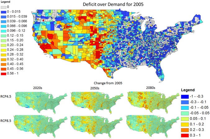
A water-deficit event occurs when the surface water available from either the locally generated runoff or accessible neighboring stream or reservoirs is insufficient to meet the required water demand on a given day. Fig. 1 shows the spatial distribution (on a county scale aggregated from results determined at a resolution of one-eighth of a degree) of average annual water deficits as a fraction of total water demand over the historical period and its relative change in three time periods under each RCP. Areas of historical surface-water deficit are predominately in the western United States and generally coincide with areas with significant irrigation or areas around urban regions. This figure also highlights the dependence of counties with large surface-water deficits on groundwater pumping and nonrenewable freshwater sources to meet their historical demands. Regions with clearly worse deficits on an average annual basis under RCP4.5 include the Great Plains region as shown in Fig. 1. As also shown, the increase in average annual water deficits in the later part of the century (Fig. 1, 2080s) is greater under the mitigation scenario (RCP4.5) than with no mitigation (RCP8.5).

Fig. 1.

Average total annual water deficit as a fraction of demand (county scale) for the historical period and the deficit difference from historical under RCP4.5 and RCP8.5 in the 2020s, 2050s, and 2080s.

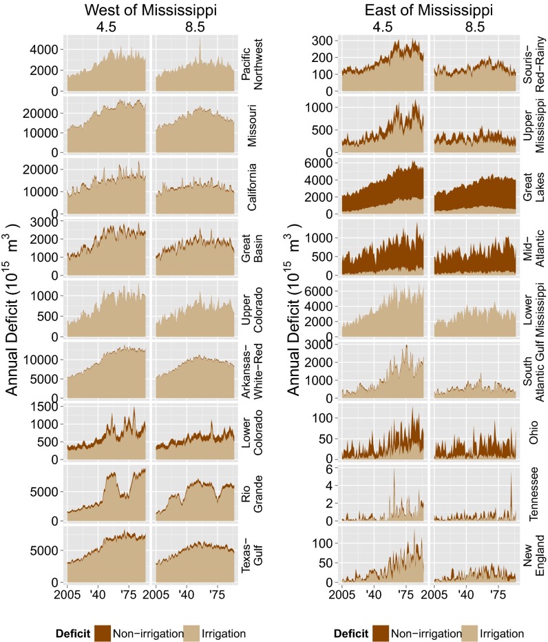
Because our approach tracks the water deficit for each water-demand sector, we can investigate how different water-demand sectors are impacted by the growing deficit and how the mix would change under mitigation vs. no mitigation scenarios. The water-demand sectors are aggregated to irrigation and nonirrigation (primarily energy and domestic) sectors. Fig. 2 shows the temporal evolution of water deficit at the annual scale for each of the water-resource regions in the United States broken into the two major categories of water-use sectors. Results clearly show that the agricultural sector will experience the majority of the deficit in total and in most basins. The nonirrigation sector dominates only in regions where there is extensive demand for power plant cooling technologies, dense population, and little irrigation requirement—primarily in the humid Northeast and parts of the Midwest.

Fig. 2.

Water deficit attributed to irrigation and nonirrigation sectors for each of the 18 basins under RCP4.5 and RCP8.5.

Projected Water-Deficit Hotspots by Major Water Basin in the United States

We define future water-deficit hotspots in each basin based on spatial and volumetric thresholds derived from the historical simulation. First, we aggregate our daily results to the monthly scale and identify grid cells with historical monthly water deficits equaling at least 10% of demand. From these grid cells, we then identify the historical 95th-percentile deficit amount as the volumetric threshold for each basin’s hotspots. This basin-specific 95th percentile value is used to identify future hotspots as grid cell clusters where the deficit of each cell is greater than the 95th percentile (see SI Materials and Methods for the detailed definition of a hotspot and for an example that shows a map of hotspots for the month of August in years 1990 and 2068 in Georgia.)

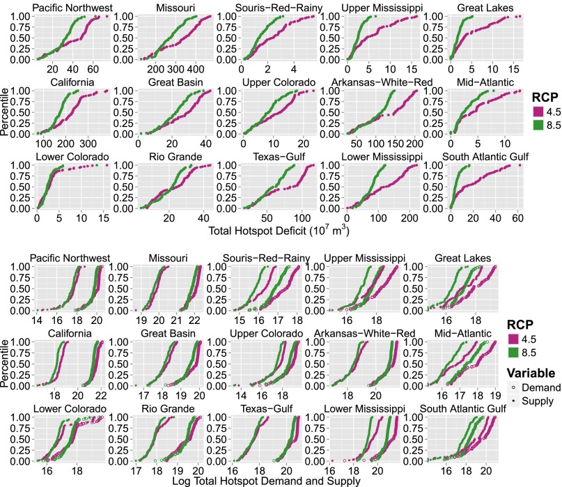
Fig. 3 shows the impact of the mitigation scenario on the volume distribution of water-deficit hotpots in each major water basin of the United States, using the high-resolution temporal (daily) and spatial (∼12 km²) outputs from our modeling system. We focus on water-deficit hotspots in August, using basin-specific 95th percentiles from August months in the historical period, because a majority of deficits peak during that time. August also is the end of the reservoir operations season for water supply and highlights the interannual variability in water storage at the end of snowmelt, shift in seasonal flow climatology, and total water demand over the summer. Fig. 3 shows a clear shift to the right of the cumulative density functions of the total deficit in all hotspots within each basin from the RCP8.5 to RCP4.5 scenarios from 2005 to 2095, suggesting that water deficits may become more severe (by volume) with mitigation. To reveal the main drivers of this deficit increase, we also present the change in water demand and supply (natural runoff) for all of the grid cells that are classified as hotspot deficits during August. Both supply and demand increase under mitigation (Fig. 3), with the latter dominating as the key driver of the increased deficits under RCP4.5 compared with RCP8.5. Water demands generally increase over time in both scenarios because of population growth and demands for food and energy and other services with consumptive use, but, as mentioned above, there is a large increase in water demands for irrigation of bioenergy crops in RCP4.5. The projected increase in water demand for bioenergy production is in agreement with other studies that found significant impacts from irrigated bioenergy crops on freshwater systems (17, 18). King et al. (19) found that water use for irrigating bioenergy crops could increase from 2% of total water consumption in 2005 to 9% in 2030 in the United States. The International Energy Agency’s Alternative Policy Scenario, which has bioenergy production increasing to 71 exajoules (EJ) in 2030, projected that the global consumptive irrigation water use for bioenergy production would increase from 0.5% of global renewable water resources in 2005 to 5.5% in 2030 (17).

Fig. 3.

Empirical cumulative density function (CDF) of total regional hotspot deficit (10⁶ m³) (top three rows) and total regional demand (solid circles) and supply (empty circles) (10⁶ m³/y) to areas categorized as deficit hotspots (bottom three rows) during the month of August for RCP 4.5 (maroon) and RCP 8.5 (green) over the period 2005–2095.

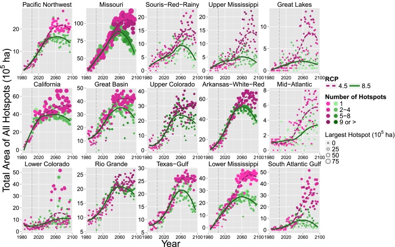
Fig. 4 provides additional insight into the results by showing the August trend over time in terms of hotspot extent, that is, the total area of grid cells that are classified as hotspots. Both hotspot extent and number increase over time under both RCPs, but the mitigation scenario leads to greater spatial coverage of areas affected by water deficit. The shape of the trend lines peaking or leveling off after midcentury is consistent with the population projection (which is the same for both scenarios), but the divergence between the two RCPs at midcentury is attributed primarily to the expansion of bioenergy crop production. When the data in Figs. 3 and 4 are combined, not only do the spatial extent and magnitude of hotspots increase under RCP4.5; both the number of occurrences and the size of the largest event also tend to increase with mitigation.

Fig. 4.

Total hotspot area (100,000 ha) in August over the time period 1985–2095 for RCP 4.5 (maroon) and RCP 8.5 (green). The size of each point is equal to the area (100,000 ha) of the largest hotspot in August of the corresponding year. The shade of the color indicates the number of hotspots in August of the corresponding year. The dashed vertical line marks the end of the historical period, 1985–2004. Trend lines were fit using LOESS.

Contrast with Other Research Results.

Our result showing that a mitigation scenario increases water deficits appears to contradict other studies such as Blanc et al. (5), Hanasaki et al. (3), and Arnell et al. (1). Aside from the work of Blanc et al. (5), which focused on the United States, all other studies provided global estimates, and several hinted about regional differences. Blanc et al. (5) concluded that adopting a climate change mitigation policy would be effective in reducing water stress for most basins in the United States, although the beneficial effect is small, and that climate policies would worsen water stress in three basins (Gila, Little Colorado, and Upper Pecos). Hanasaki et al. (3) performed a comprehensive global analysis of the effects of climate change under the various RCP scenarios and shared socioeconomic scenarios. Arnell et al. (1) also investigated the potential effect of climate policy on the impacts of climate change on exposure to water resources stress globally. They found that their mitigation policy scenario (CO₂ stabilized to 450 ppm by 2100) would reduce the population exposed to water stress by 5–21% in 2050, by 13–40% in 2080, and by 15–47% in 2100. Thus, they concluded that climate policy could prevent less than half of the potential impacts of climate change, with little effect before the middle of the 21st century. The opposing results can be attributed to differences in the underlying assumptions pertaining to the water-demand sectors, input climate information, the hydrologic model used and the structural differences in models, the spatial and temporal resolutions of the modeling and analysis, and the adopted mitigation options, among others.

To investigate the implications of spatial and temporal resolutions (a distinguishing feature of our modeling) on the water-deficit results, we have reassessed the total annual deficit at multiple spatial and temporal scales for each of the two RCPs. More specifically, we compared the evolution of the annual deficit by aggregating the natural streamflow and demands from the daily scale and a resolution of one-eighth of a degree against four alternative methods: (i) aggregating from daily to monthly to compute monthly deficits aggregated to annual at a resolution of one-eighth of a degree; (ii) aggregating to an annual scale to compute annual deficits directly at a resolution of one-eighth of a degree; (iii) as in the first method, but aggregating to a resolution of one-half of a degree; and (iv) as in the second method but aggregating to a resolution of one-half of a degree. All results then are compiled for the whole United States by summing up the total annual deficits from all grids. Fig. 5 clearly shows that by computing deficits at coarser spatial and temporal scales we significantly underestimate the amount of deficits, simply because of the averaging effect of the inherent spatial and temporal variability of natural streamflow and water demands. The results also clearly show the divergence between the two RCP scenarios around midcentury. However, that difference (or signal) tends to diminish as we move to coarser temporal and spatial scales. Fig. 5 also shows that the signal-to-noise ratio diminishes at coarser scales during 2065–2094, perhaps explaining the mixed results in previous studies. For example, Arnell et al. (1) and Hejazi et al. (4) computed water scarcity at the annual scale and at a spatial resolution of one-half of a degree. Akimoto et al. (2) computed water scarcity at the annual scale and at a spatial resolution of one-fourth of a degree. Hanasaki et al. (3) performed a daily assessment of water deficit at a spatial resolution of one-half of a degree. Blanc et al. (5) calculated water deficit at the monthly and annual scales with a relatively coarse spatial resolution of 2 × 2.5 degrees and mapped to the basin scale.

Fig. 5.

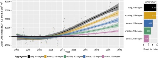
(Left) The difference in total annual water deficit between the two RCP scenarios (RCP4.5 minus RCP8.5) using multiple methods of aggregations both spatially and temporally; shaded areas represent the 95% confidence band on the mean trend. (Right) A comparison of signal-to-noise ratios across the five aggregation methods and the future time period of 2065–2094.

Our study also takes advantage of a global assessment model that is extended to model the economic decisions at much finer spatial scales (states) than most other IAMs and is coupled to a high-resolution regional ESM with state-of-the-art river routing (20) and reservoir operations models (21). Akimoto et al. (2) and Hejazi et al. (4) did not include representations of reservoirs or river routing. Blanc et al. (5) allocated water using a single virtual reservoir for each basin and routed water laterally by assuming that unused upstream water is made available to the basin directly downstream. Hanasaki et al. (3) included only the largest 507 reservoirs globally, compared with the 1,848 reservoirs in the United States used in our study. Also, most previous studies used IAMs that treat the whole United States as a single region, thus losing important details about regional differences. This study relies on a single global and regional climate model, a single regional IAM, and a single socioeconomic pathway to achieve the mitigation target. However, the seasonal and spatial patterns of wet/dry trends from the global and regional models are broadly consistent with the Coupled Model Intercomparison Project Phase 5 (CMIP5) multimodel ensemble (22). The study also assumes that all water demands are abstracted from internally generated runoff, neighboring rivers, and reservoirs, thus excluding groundwater sources. This assumption does not alter the conclusion that water deficits are more pronounced under mitigation. This study also uses the same shared socioeconomic pathway (SSP) assumptions (i.e., SSP5) under RCP4.5 and RCP8.5 to ensure a consistent comparison between the two RCP scenarios and because RCP8.5 is unachievable under the other four SSPs. The fact that there are multiple socioeconomic pathways (23) to stabilize at 4.5 W/m² does not alter the conclusion that when the socioeconomic inputs are kept constant between the two RCPs, climate change mitigation exacerbates water stress. Future research should investigate the reproducibility of the results when using other regional ESMs, regional IAMs, and SSPs.

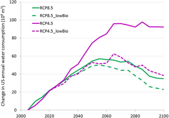
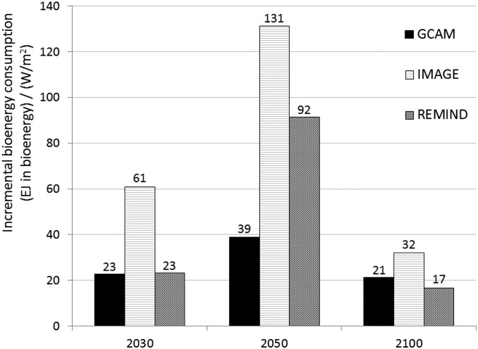
Replicating the two RCP scenarios with a prescribed low bioenergy consumption target in year 2100 (e.g., 45 EJ, the lowest among six IAMs in the AR5 Scenario Database; https://secure.iiasa.ac.at/web-apps/ene/AR5DB) and favoring other renewables in mitigating emissions to achieve RCP4.5, the annual water consumption in the United States still increases under RCP 4.5 as compared with RCP8.5, although the magnitude of the increase is reduced from 42% to 12%. The lower difference can be depicted as the lower bound, and, depending on the rate at which bioenergy consumption increases under mitigation, this gap is likely to increase when bioenergy is unconstrained. The lower difference also suggests that the climate benefit of mitigation can be realized for temperature and water stress if designed carefully toward less water-intensive mitigation options. However, bioenergy is considered a cost-effective mitigation option, and IAMs generally observe more bioenergy production under mitigation. For example, in a large intermodel comparison of 15 IAMs, mitigation is found to increase bioenergy deployment and reliance in all models (24). Also constraining bioenergy restricts the opportunity for negative emissions in the long term, thus requiring more aggressive near-term emissions reductions, which has implications for mitigation and macroeconomic costs of climate policies (24). Still, the tendency to introduce more bioenergy consumption under mitigation than a under a reference (no policy) scenario is consistent with other IAMs (25). For example, the rate of increase in bioenergy consumption per unit of reduced radiative forcing in year 2100 is 21, 17, and 32 EJ⋅W⁻¹⋅m⁻² for the Global Change Assessment Model (GCAM), the Regional Model of Investments and Development (REMIND), and the Integrated Model to Assess the Global Environment (IMAGE), respectively (EMF27 scenario database; https://secure.iiasa.ac.at/web-apps/ene/AR5DB/). Thus, the use of other IAMs is unlikely to change the conclusion that water demands increase under mitigation.

By coupling enhanced, higher-resolution human and natural systems models, we are able to identify potential interactions and constraints that could not be seen with earlier modeling systems and reveal important policy implications. That is, climate change mitigation policies designed to mitigate greenhouse gas emissions may exacerbate water stresses across the United States and potentially limit the ability to achieve mitigation goals that rely on water availability (e.g., to grow bioenergy crops). Understanding potential synergies and/or constraints for mitigation policy within the climate–energy–water nexus and fostering water-efficient technologies in the energy and agricultural sectors remain national priorities.

SI Materials and Methods

The WM Model.

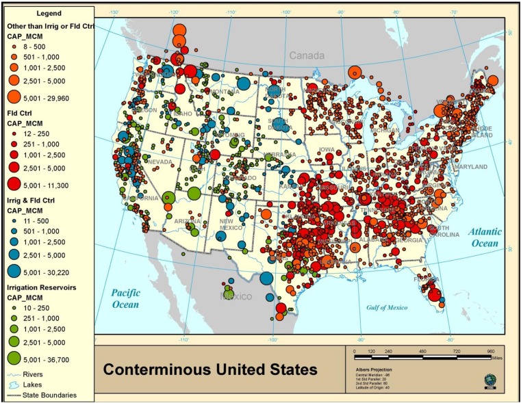
A large-scale reservoir operations model (WM) with a daily representation at a resolution of one-eighth of a degree is used to allocate water demands and manage reservoir releases and storage. The 1,848 reservoirs that are explicitly modeled in this study are broken by their primary use into four categories (flood control, irrigation, flood control with irrigation, and others) as shown in Fig. S1.

Fig. S1.

Spatial distribution of all modeled reservoirs in this study; the color indicates the primary use of the reservoir, and the size of the circle indicates its storage capacity.

Downscaling of Water Demands for Electricity Generation.

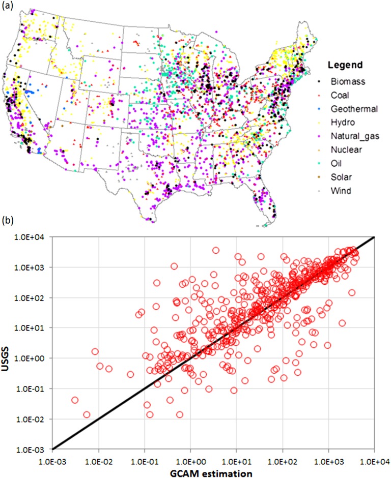
Using a database recently compiled by the Union of Concerned Scientists of power plant locations in United States with extensive information including the geographic location, built year, consumed fuel type, adopted generation technology, cooling technology, and the source of cooling water (41), an enhanced algorithm for spatially downscaling electricity water use from the state level to the grid scale (original method documented in refs. 15 and 4) is implemented. The power plants are broken by fuel types (coal, nuclear, natural gas, biomass, solar, wind, geothermal, hydropower, and oil; see Fig. S2A), generation technologies (combustion turbine, combined cycle, and generic steam), and cooling technologies (once-through, recirculating, cooling pond, and dry-cooled). By downscaling the water-demand results for year 2005 to the grid level and then aggregating to county level, we compare our estimation with US Geological Survey (USGS) inventory for 2005 at the county level (Fig. S2B). Moving forward in time and for new power plants, we assume the new loads will be distributed to all the existing power plants locations, regardless of their cooling technologies and generation technologies.

Fig. S2.

(A) Spatial distribution of all power plant locations in the United States by fuel type. (B) scatter-plot comparison between the estimated electricity water withdrawal by GCAM and USGS statistics at the county level.

Calculations of Hotspots.

Future occurrences of extreme water deficit are of great interest, especially when these events occur in areas within close proximity to one another. We introduce a method to identify collocated areas with extreme water deficit at a fixed point in time by defining hotspots of water deficit. A deficit hotspot is defined as a group of adjacent cells each exceeding a deficit threshold. The minimum number of adjacent cells for a group of cells to be considered a hotspot and the deficit threshold that an individual cell must exceed are quantities that may be set to values of interest to the researcher. This methodology not only identifies areas of interest; it also allows extreme deficit behavior to be described quantitatively with statistics that characterize the severity of water deficit in terms of magnitude, spatial extent, and temporal changes.

Here we implement the hotspot algorithm on the monthly water-deficit values over cells on the one-eighth of a degree grid for each of the 18 basins separately. For this study we investigated hotspot behavior for the month of August, over time, and excluded cells that do not have demand throughout all years. For this analysis, we require a minimum of four adjacent cells exceeding the deficit threshold for an area to be identified as a deficit hotspot (for an example see Fig. S3). The threshold value for a deficit was determined for each basin using data from the historical period. In determining thresholds, we consider all deficit values from August months in the historical period. Because we are interested primarily in deficits that are nontrivial with respect to the demand, we limited our calculations to include only values where the deficit is at least 10% of demand. Given the deficit values that meet these criteria, we use the 95th percentile from the distribution of deficit values, by basin, as the threshold value of interest in this investigation. Table S1 gives the threshold values for each basin.

Fig. S3.

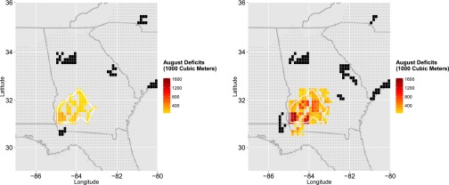
An example of a hotspot water-deficit event in the state of Georgia in August 1990 (Left) and 2068 (Right).

Table S1.

Hotspot deficit threshold values for each basin based on the 95th percentile

Basin	Threshold, m3
Tennessee	40,469.91
Souris–Red–Rainy	161,718.64
Lower Colorado	163,323.86
Ohio	272,820.91
New England	394,732.65
Upper Colorado	402,967.25
Upper Mississippi	491,756.19
Rio Grande	550,919.28
Great Basin	559,606.85
South Atlantic Gulf	796,154.63
Great Lakes	908,527.79
Mid-Atlantic	1,452,178.59
Pacific Northwest	2,087,591.02
Arkansas–White–Red	2,307,534.01
Missouri	2,451,318.30
Texas–Gulf	3,362,109.23
Lower Mississippi	3,756,925.35
California	4,695,288.15

The hotspot algorithm was run on deficit data for both RCP 4.5 and 8.5. In addition to identifying hotspots for a given month within a basin, several summary statistics, including number of hotspots, size (or area) of the largest hotspot, and total deficit over all hotspots, were calculated.

Low Bioenergy Scenarios.

To address the sensitivity of the results to the choice of IAM and to the rate at which bioenergy is used to mitigate emissions, two additional scenarios that assume low bioenergy expansion in the future were conducted. The low bioenergy scenario was taken from the AR5 Scenario Database (https://secure.iiasa.ac.at/web-apps/ene/AR5DB) following the lowest trajectory for bioenergy consumption among six IAMs [IMAGE, MERGE (Model for Evaluating Regional and Global Effect), MESSAGE (Model for Energy Supply Strategy Alternatives and their General Environmental Impact), SGM (Second Generation Model), TIAM (Time-Integrated Assessment Model)-World, and WITCH (World Induced Technical Change Hybrid)] for RCP4.5. Fig. S4 shows that the difference in the annual water consumption in the United States decreases from 42% to 12% when constraining bioenergy consumption for both RCP scenarios. Fig. S5 shows that GCAM is consistent with other IAMs (IMAGE and REMIND) in terms of the incremental increase in bioenergy consumption per 1 W/m² in mitigation. The rates were estimated by using results from the EMF27 Scenario database (https://secure.iiasa.ac.at/web-apps/ene/AR5DB) for a reference and CO₂ emission stabilization at 550 ppm (3.7 W/m²) scenarios.

Fig. S4.

Changes in annual water consumption in the United States from 2005 estimates under the RCP4.5 and RCP8.5 scenarios (solid lines) and two additional replicated scenarios with a prescribed low trajectory of bioenergy consumption by the end of the 21st century (dashed lines).

Fig. S5.

Rates of increase in bioenergy consumption resulting from mitigating emissions by 1 W/m² in three time periods (2030, 2050, 2100) and using three IAMs (GCAM, IMAGE, REMIND).

Materials and Methods

This research used an integrated regional modeling framework proposed by Hibbard and Janetos (26) and further described by Kraucunas et al. (27). The framework, the Platform for Regional Integrated Modeling and Analysis (PRIMA), integrates a regional ESM with a regional IAM and detailed sector models using consistent global climate and socioeconomic scenarios. The framework is executed over a historical period and into the future under the RCP4.5 and RCP8.5 scenarios. The Regional Earth System Model (RESM) (28, 29) was applied to a North American domain at 20-km grid resolution driven by large-scale circulation and sea surface temperature provided by the Community Earth System Model (CESM) from the CMIP5 archive (22). Downscaling was performed for 1975–2004 (historical) and 2005–2100 (future) using CESM boundary conditions for the historical run and the RCP4.5 and RCP8.5 scenarios. The RESM simulations were postprocessed using bias correction to provide meteorological forcing for offline simulations using version 4 of the Community Land Model (CLM) (30) at a resolution of one-eighth of a degree. The bias correction followed the method described by Wood et al. (31). Data input to CLM, such as land cover, soil properties, and vegetation phenology, were retrieved from datasets developed by Ke et al. (29) at a resolution of 0.05° and were aggregated to a resolution of one-eighth of a degree. CLM was spun up by recycling the meteorological forcing over the historical period (1975–2004) until all state variables, including soil moisture, soil temperature, and groundwater table depth, reached equilibrium. Then the model was forced by the two bias-corrected RESM downscaled climate scenarios, RCP4.5 and RCP8.5, to simulate terrestrial hydrological states and fluxes from 2005–2100. Runoff is routed spatially using a physically based river-routing model, the Model for Scale Adaptive River Transport (MOSART). Surface runoff first is routed across hill slopes and then is discharged along with subsurface runoff into a “tributary subnetwork” before entering the main channel (20, 32). A water-management (WM) model is used to allocate water demands and manage reservoir releases. The WM model relies on generic operating rules that mimic monthly release patterns based on the objective of the reservoir (flood control with irrigation and others) (13, 21). The WM model is coupled to MOSART to route the regulated flow from reservoirs to downstream channels. CLM, MOSART, and the WM model are all applied at a grid resolution of one-eighth of a degree. Water demands are taken from GCAM for the United States (GCAM-USA) described below.

This study uses the regionalized version of the GCAM-USA (33, 34) with the 50 states plus the District of Columbia as explicit regions that operate within the global GCAM model (35). Energy transformation (electricity generation and refined liquids production) and end-use demands (buildings, transportation, and industry) are modeled at the individual state level. In addition state-specific characterization is given for renewable energy (wind, central and rooftop photovoltaic, concentrated solar power, and geothermal) and carbon storage potential. To replicate the RCP4.5 and RCP8.5 scenarios in which radiative forcing stabilizes at 4.5 W/m² or exceeds 8.5 W/m² by the end of the century, a modified version of SSP5 (23) was chosen as the basis for the socioeconomic assumptions. For the GCAM-USA RCP4.5 replication, we started with the same scenario assumptions as for the RCP8.5 scenario and introduced a carbon policy to meet the mitigation goal. Although there are multiple shared SSPs (23) to achieve RCP4.5, we used SSP5 for both RCPs to ensure a fair comparison between the two RCPs.

GCAM-USA accounts for the impacts of climate change on building energy use and crop yields. The climate change impact on building energy use was evaluated using a detailed, service-based buildings energy model at the 50-states level (34) nested in the GCAM-USA modeling framework. The evolution of energy demand in the building sector and its interactions with climate change were explored by constructing estimates of population-weighted heating and cooling degree days (HDD/CDDs) for both the RCP4.5 and RCP8.5 scenarios built from the RESM model output. Similarly, to model climate change impacts on crop yields and agricultural markets globally, we used the output of a global gridded crop model, the GIS-based Environmental Policy Integrated Climate (GEPIC) model (36), which in turn was driven by climate data from a global climate model, The Norwegian Earth System Model (NorESM) (37), for the two emissions pathways analyzed in this study (8.5 W/m² and 4.5 W/m²). Climate change impacts on yields are aggregated to GCAM’s 151 agricultural regions and expanded from the available crops in GEPIC as documented in Kyle et al. (38) to calculate yield adjustment factors for each of GCAM’s crops, agricultural regions, and time periods. These adjustment factors then are applied to the baseline assumptions of agricultural productivity change by crop and region derived from the Food and Agriculture Organization of the United Nations database described by Bruinsma (39).

GCAM-USA includes a detailed representation of six water-demand sectors (irrigation, livestock, municipal, electricity generation, primary energy, and manufacturing water demands) and tracks them at multiple spatial scales and annual scale (4, 40). A spatial and temporal disaggregation approach was developed to project the United States annual regional water-demand simulations into a daily time step and a spatial resolution of one-eighth of a degree. The downscaled products were used as inputs to CLM-MOSART-WM, and the work was demonstrated over the United States Midwest region in Voisin et al. (13). Dependency maps specifying the possible sources of water for each grid were constructed based on a suite of suitable calipers. The estimates of water deficits were compiled at a daily scale. When the demand in a grid at a particular day cannot be met in full by local and remote sources, the unmet demand amount is denoted as a water deficit. A hotspot is defined as a minimum of four contiguous grids exhibiting a water deficit that exceeds 10% of the total water demand. Thus, a hotspot may be much larger than four grids in spatial extent, and generally many hotspot events occur in a basin in a given month.

References

- 1.Arnell N, van Vuuren D, Isaac M. The implications of climate policy for the impacts of climate change on global water resources. Glob Environ Change. 2011;21(2):592–603. [Google Scholar]
- 2. Akimoto K, et al. (2012) Consistent assessments of pathways toward sustainable development and climate stabilization. Nat Resour Forum 36(4):231–244.
- 3. Hanasaki N, et al. (2013) A global water scarcity assessment under Shared Socio-economic Pathways: Part 2 Water availability and scarcity. Hydrol Earth Syst Sci 17:2393–2413. [Google Scholar]
- 4. Hejazi MI, et al. (2014) Integrated assessment of global water scarcity over the 21st century under multiple climate change mitigation policies. Hydrol Earth Syst Sci 18:2859–2883.
- 5. Blanc E, et al. (2014) Modeling U.S. water resources under climate change. Earths Futur 2(4):197–224.
- 6. Huntington T (2006) Evidence for intensification of the global water cycle: Review and synthesis. J Hydrol (Amst) 319:83–95.
- 7.Wentz FJ, Ricciardulli L, Hilburn K, Mears C. How much more rain will global warming bring? Science. 2007;317(5835):233–235. doi: 10.1126/science.1140746. [DOI] [PubMed] [Google Scholar]
- 8.Milly PC, Dunne KA, Vecchia AV. Global pattern of trends in streamflow and water availability in a changing climate. Nature. 2005;438(7066):347–350. doi: 10.1038/nature04312. [DOI] [PubMed] [Google Scholar]
- 9.Milly PC, Wetherald RT, Dunne KA, Delworth TL. Increasing risk of great floods in a changing climate. Nature. 2002;415(6871):514–517. doi: 10.1038/415514a. [DOI] [PubMed] [Google Scholar]
- 10.Sherwood S, Fu Q. Climate change. A drier future? Science. 2014;343(6172):737–739. doi: 10.1126/science.1247620. [DOI] [PubMed] [Google Scholar]
- 11.Oki T, Kanae S. Global hydrological cycles and world water resources. Science. 2006;313(5790):1068–1072. doi: 10.1126/science.1128845. [DOI] [PubMed] [Google Scholar]
- 12.Vörösmarty CJ, Green P, Salisbury J, Lammers RB. Global water resources: Vulnerability from climate change and population growth. Science. 2000;289(5477):284–288. doi: 10.1126/science.289.5477.284. [DOI] [PubMed] [Google Scholar]
- 13. Voisin N, et al. (2013) One-way coupling of an integrated assessment model and a water resources model: Evaluation and implications of future changes over the US Midwest. Hydrol Earth Syst Sci 17:4555–4575.
- 14.van Vuuren DP, et al The representative concentration pathways: An overview. Clim Change. 2011;109(1-2):5–31. [Google Scholar]
- 15. Riahi K, et al. (2011) RCP 8.5—A scenario of comparatively high greenhouse gas emissions. Clim Change 109(1-2):33–57.
- 16. Thomson AM, et al. (2011) RCP4.5: A pathway for stabilization of radiative forcing by 2100. Clim Change 109(1-2):77–94.
- 17.Gerbens-Leenes P, van Lienden A, Hoekstra A, van der Meer T. Biofuel scenarios in a water perspective: The global blue and green water footprint of road transport in 2030. Glob Environ Change. 2012;22(3):764–775. [Google Scholar]
- 18.Jacobson M. Review of solutions to global warming, air pollution, and energy security. Energy Environ Sci. 2009;2(2):148–173. [Google Scholar]
- 19.King C, Webber M, Duncan I. The water needs for LDV transportation in the United States. Energy Policy. 2010;38(2):1157–1167. [Google Scholar]
- 20. Li H-Y, et al. (2013) A physically based runoff routing model for land surface and Earth system models. J Hydrometeorol 14(3):808–828.
- 21. Voisin N, et al. (2013) On an improved sub-regional water resources management representation for integration into earth system models. Hydrol Earth Syst Sci 17:3605–3622.
- 22. Gao Y, et al. (2014) Robust spring drying in the southwestern US and seasonal migration of wet/dry patterns in a warmer climate. Geophys Res Lett 41(5):1745–1751.
- 23. O’Neill BC, et al. (2014) A new scenario framework for climate change research: The concept of shared socioeconomic pathways. Clim Change 122(3):387–400.
- 24. Rose SK, et al. (2014) Bioenergy in energy transformation and climate management. Clim Change 123(3-4):477–493.
- 25. Popp A, et al. (2014) Land-use transition for bioenergy and climate stabilization: Model comparison of drivers, impacts and interactions with other land use based mitigation options. Clim Change 123(3-4):495–509.
- 26.Hibbard K, Janetos A. The regional nature of global challenges: A need and strategy for integrated regional modeling. Clim Change. 2013;118(3-4):565–577. [Google Scholar]
- 27. Kraucunas IP, et al. (2014) Investigating the nexus of climate, energy, water, and land at decision-relevant scales: The Platform for Regional Integrated Modeling and Analysis (PRIMA). Clim Change 129(3-4):573–588.
- 28.Leung L, Kuo Y-H, Tribbia J. Research needs and directions of regional climate modeling using WRF and CCSM. Bull Am Meteorol Soc. 2006;87(12):1747–1751. [Google Scholar]
- 29. Ke Y, et al. (2012) Development of High Resolution Land Surface Parameters for the Community Land Model. Geoscientific Model Development 5(6):1341–1362.
- 30. Oleson KW, et al. (2010) Technical Description of version 4.0 of the Community Land Model (CLM). NCAR Technical Note NCAR/TN-478+STR (National Center for Atmospheric Research, Boulder, CO), 257 pp.
- 31.Wood A, Leung L, Sridhar V, Lettenmaier D. Hydrologic implications of dynamical and statistical approaches to downscaling climate model outputs. Clim Change. 2004;62(1-3):189–216. [Google Scholar]
- 32. Li et al. (2014) Evaluating global streamflow simulations by a physically-based routing model coupled with the Community Land Model. J Hydrometeorol 16(2):948–971.
- 33. Liu L, et al. (2015) Water demands for electricity generation in the US: Modeling different scenarios for the water–energy nexus. Technol Forecast Soc Change 94:318–334.
- 34. Zhou Y, et al. (2014) Modeling the effect of climate change on U.S. state-level buildings energy demands in an integrated assessment framework. Appl Energy 113:1077–1088.
- 35.Edmonds J, Reilly J. A long-term, global, energy-economic model of carbon dioxide release from fossil fuel use. Energy Econ. 1983;5(2):74–88. [Google Scholar]
- 36. Liu J, et al. (2007) GEPIC – modeling wheat yield and crop water productivity with high resolution on a global scale. Agric Syst 94(2):478–493.
- 37. Bentsen M, et al. (2013) The Norwegian Earth System Model, NorESM1-M – Part 1: Description and basic evaluation. Geosci. Model Dev. 6:687–720.
- 38.Kyle P, Müller C, Calvin K, Thomson A. Meeting the radiative forcing targets of the representative concentration pathways in a world with agricultural climate impacts. Earths Futur. 2014;2(2):83–98. [Google Scholar]
- 39.Bruinsma J. The Resource Outlook to 2050: By how Much Do Land, Water, and Crop Yields Need To Increase by 2050? Expert Meeting on How to Feed the World in 2050? Food and Agriculture Organization of the United Nations; Rome: 2009. [Google Scholar]
- 40. Hejazi MI, et al. (2014) Long-term global water use projections using six socioeconomic scenarios in an integrated assessment modeling framework. Technol Forecast Soc Change 81:205–226.
- 41. Averyt K, et al. (2011) Freshwater Use by U.S. Power Plants: Electricity’s Thirst for a Precious Resource (Union of Concerned Scientists, Cambridge, MA)