

Significance
The US Great Plains is an agricultural production center for the global market and a source of greenhouse gas (GHG) emissions. This article uses historical data and ecosystem models to estimate the magnitude of annual GHG fluxes from all agricultural sources (cropping, livestock, irrigation, fertilizer production, and tractor use) from 1870 to 2000. Carbon (C) emissions from plow-out of native grasslands peaked in the 1930s and were the largest agricultural source of GHG emissions at the time. Soil C emissions subsequently declined, whereas GHG fluxes from other activities increased. The results inform knowledge about the relationship between agriculture and its environmental setting and show that available alternative management practices could substantially mitigate the environmental consequences of agricultural activities without reducing food production.
Keywords: modeling, Great Plains, biogeochemistry, greenhouse gases, agricultural management
Abstract
The Great Plains region of the United States is an agricultural production center for the global market and, as such, an important source of greenhouse gas (GHG) emissions. This article uses historical agricultural census data and ecosystem models to estimate the magnitude of annual GHG fluxes from all agricultural sources (e.g., cropping, livestock raising, irrigation, fertilizer production, tractor use) in the Great Plains from 1870 to 2000. Here, we show that carbon (C) released during the plow-out of native grasslands was the largest source of GHG emissions before 1930, whereas livestock production, direct energy use, and soil nitrous oxide emissions are currently the largest sources. Climatic factors mediate these emissions, with cool and wet weather promoting C sequestration and hot and dry weather increasing GHG release. This analysis demonstrates the long-term ecosystem consequences of both historical and current agricultural activities, but also indicates that adoption of available alternative management practices could substantially mitigate agricultural GHG fluxes, ranging from a 34% reduction with a 25% adoption rate to as much as complete elimination with possible net sequestration of C when a greater proportion of farmers adopt new agricultural practices.
As the extent and role of greenhouse gases (GHGs) in climate change increase in importance, the need for more refined estimates has grown. In addition, improved estimates of specific economic sectors, with better temporal and spatial detail, have become critical. This need is especially acute for agriculture because it is dispersed spatially throughout the world and has contributed GHGs over a long period, although with variation through time, and also across space. In this paper, we describe GHG fluxes from all types of agriculture in the US Great Plains from 1870 to 2000, based on innovative estimates made at the county level for cropping, use of inputs and equipment, and livestock production. The results show two long-term trends. The trend for cropping [measuring changes in carbon (C), nitrogen (N) release, and methane (CH4) uptake] shows that GHG release, measured as gigagrams (Gg) of carbon dioxide (CO2)-carbon equivalent (Ce), peaked in the 1930s and has substantially declined since. The trend for livestock production, agricultural inputs, and equipment use reveals long-term growth in GHG fluxes, reflecting changes in the size and structure of livestock herds in the Great Plains, plus an increased use of synthetic fertilizers, irrigation, and tractors. In the context of US GHG production as a whole (as estimated by the annual GHG inventory of the US Environmental Protection Agency) (1), we estimate that the Great Plains contributes less than 5% of US agricultural GHGs. Nonetheless, this analysis provides important information about the relationship between agricultural practices, the environmental setting of those practices, and the GHG consequences of agriculture in a large region, which is useful for consumers, producers, and policy makers alike.
The US Great Plains is a globally important agricultural region, providing both the US and world economies with grain, fiber, and meat. This region contains more than 30% of the US agricultural land area, and accounts for more than 50% of winter wheat and more than 30% of beef production in the country. The Great Plains region is located in the central United States, generally west of the 98th meridian and east of the Rocky Mountains (Fig. 1). The semiarid temperate climate of this region encompasses enormous subregional diversity, reflected in mean annual temperatures ranging from more than 20 °C in Texas to less than 0 °C in North Dakota, with annual precipitation levels ranging from 700 to 200 mm along an east-west gradient. The native vegetation is primarily grassland, with mixed-grass prairie in the east and shortgrass steppe in the west (3, 4).
Fig. 1.

Irrigation in the US Great Plains. Counties shaded in light blue irrigated at least 25% of cropland area in 2007; in the unshaded counties, dryland cropping accounts for 75% or more of cropland (2).
Agricultural production in the Great Plains increased dramatically between 1870 and 2000, facilitated by changes in farming techniques, all of which have led to significant GHG releases. Historically, soil cultivation has represented the largest agricultural source of GHGs, producing both C (30–50% soil C losses) and nitrous oxide (N2O) (5). N mineralization rates, enhanced by cropping, increase the N2O released from the soil, with the application of N fertilizer causing further N2O emissions (6). The other major sources of GHGs include CH4 from cattle and other livestock production (7); fossil fuels used in fertilizer production; and C released from burning of fossil fuels by tractors, irrigation pumps, and other farm equipment.
Agricultural GHG production in the Great Plains is also tightly tied to public policy actions, primarily those of the US government. The plow-out of the plains would not have been as rapid without the Homestead Act of 1862, which distributed land at no cost to those homesteaders willing to cultivate it. In addition, the 20th century reduction in the extent of cropland (described later) was spurred by agricultural support policies that arose out of the economic and climatic events of the 1930s and are still in existence, in various forms, today.
Previous studies of the GHG fluxes associated with agriculture in North America and Europe have used field measurements (8, 9), inventory methods (10), economic land use models (e.g., the “Forest and Agricultural Sector Optimization Model with Greenhouse Gases”) (11, 12) or ecosystem models (e.g., the Daycent model used here) (13, 14) to estimate GHG sources or sinks at either the present time or at specific points in the past or future. Although some methods estimate future GHG fluxes under projected scenarios (14, 15) and others compare the GHG production of current and past agricultural production systems (10, 13), no previous study has estimated cumulative GHG emissions from all agricultural sources from initial plow-out to the present.
The historical and complete perspective offered by this article provides important insights into the environmental impact of agriculture. First, the magnitude of GHG emissions is a result not just of land use practices but also of land use change, which is not captured by synchronic analysis (8). Second, the soil GHG flux at any point in time depends on the previous land use history (8, 12, 16, 17). Third, some practices that enhance soil C sequestration, such as fertilizer application and irrigation, increase GHG emissions from N2O release and fossil fuel burning (9, 18). This paper estimates GHG fluxes from “on-farm” activities, and also includes the energy used for irrigation pumping, tractors, and the production of synthetic fertilizer. The Daycent ecosystem model was used to estimate soil GHG fluxes associated with cropping in each of 476 Great Plains counties (19). A complete description of the procedure used to estimate all of the GHG fluxes is provided in SI Materials and Methods.
SI Materials and Methods
The region of the US Great Plains used in this study is composed of 476 counties in 12 states (Colorado, Iowa, Kansas, Minnesota, Montana, Nebraska, New Mexico, North Dakota, Oklahoma, South Dakota, Texas, and Wyoming), each of which receives less than 700 mm of annual rainfall, has an average elevation less than 5,000 feet, and lies north of the 32nd parallel. We describe here the method by which GHG fluxes from each agricultural source were first estimated at the county level and then aggregated to produce estimates for the whole Great Plains region. Fig. S1 illustrates the relationship between the major sources of agricultural GHG emissions with (i) C flux, N2O release, and CH4 uptake by the soil; (ii) C burned during N fertilizer production, tractor use, and irrigation pumping; and (iii) CH4 released by livestock. We conclude by examining existing agricultural management practices that have the potential to reduce GHG emissions from Great Plains agricultural systems.
Fig. S1.

Schematic illustrating the various sources of agricultural GHG flux in the US Great Plains, and the data and methods used to estimate them.
Historical Changes in Great Plains Land Use.
This process began with the selection of 21 counties to represent the ecosystem diversity and variety of cropping practices in the US Great Plains (19). For each of these representative counties, a set of schedule files was created to detail daily agricultural events for all major dryland and irrigated cropping systems between 1870 and 2000. These schedules capture historical changes in land use, including initial plow-out and the introduction of irrigation and new crop rotations when appropriate. Within each county, replicate schedule files stagger rotations to simulate crop growth in each year, with a variance in the date of first cultivation among these files to capture the progressive plow-out of native prairie. Additional schedule files represent land never cropped (pasture), cropland removed from production between 1950 and 1975 (return), and cropland enrolled in the CRP (41) after 1985. Fig. S2 illustrates the set of schedule files developed for one of the 21 representative counties. Schedule files also include (i) changes in crop variety; (ii) dates and intensity of cultivation events; (iii) dates of planting, harvesting, and irrigation; and (iv) dates and amounts of crop residue removal and fertilizer application. These files serve as input to the Daycent model, which estimates soil GHG fluxes, yet the information embedded in them also allows for the calculation of GHG emissions from tractor use, irrigation pumping, and N fertilizer production.
Fig. S2.

Schematic showing the 12 schedule files created to represent cropping in Baca County, CO between 1870 and 2000.
Schedule files were calibrated by (i) running the Daycent model, (ii) comparing the time series of simulated yields for major crops with the time series of yields reported in the USDA Census of Agriculture (20) and the USDA National Agricultural Statistics Service database (www.nass.usda.gov), and (iii) adjusting schedule parameters to increase the correspondence between simulated and observed yields. Adjustments included (i) adding or removing fertilizer, (ii) increasing or decreasing crop residue removal, (iii) increasing or decreasing cultivation intensity and frequency, and (iv) changing crop variety, all within historically realistic limits. After calibration, schedule files were verified for the 21 representative counties by calculating measures of fit between observed and simulated yields. A validation process then tested the capability of these schedule files to represent agriculture in other Great Plains counties: Dryland and irrigated wheat and corn rotation schedule files for 20 of the 21 representative counties were run using weather and soil data for the county directly to the north (Cherry, NE has no validation county), and the same measures of fit between observed and simulated yields were computed for the validation counties. These measures of fit declined only slightly between verification and validation runs, demonstrating the generalizability of the schedule files developed for the 21 representative counties to other nearby counties. More information about Daycent calibration and validation methods, including measures of fit for verification and validation runs, can be found in the study by Hartman et al. (19).
To use these 21 sets of schedule files to represent cropping in all 476 Great Plains counties, the region was divided into 21 county clusters, each containing one of the 21 representative counties. This process involved (i) running an exploratory average means cluster analysis (k-means in Stata; StataCorp) for all 476 counties (variables included latitude and longitude of county centroid, elevation, mean annual precipitation and temperature, and measures of land use reported in recent agricultural censuses), which generated 14 clusters; (ii) reassigning counties as needed to make clusters contiguous and to group together counties with similar agricultural practices; (iii) dividing clusters to ensure that each contained one, and only one, of the 21 representative counties; and (iv) creating an index of dissimilarity [based on the methods used by Weaver (61)] to test and refine cluster assignments. This index was computed for each county by subtracting the proportion of land in each crop (averaged over two time periods, 1880–1945 and 1950–2002) from the same proportion in the relevant representative county, squaring the differences, summing over crops and time periods, and multiplying by 100. Dissimilarity between a representative county and any of the other counties in its cluster had a minimum value of zero (for the 21 representative counties) and a maximum value of 138. Forty-nine counties (just over 10%) had a dissimilarity value greater than 50. These counties were reassigned if, and only if, doing so would both improve their dissimilarity score and preserve the contiguity of the clusters. After reassignment, only two counties still had dissimilarity scores over 50.
The schedule files developed for each of the 21 representative counties were then extended to all of the other counties in the cluster, with the land in each county divided among those files. All counties in a cluster used the same set of schedule files, but the distribution of land among those files differed by county. Land in each county was allotted to schedules using the following quantities from the 1880–2007 censuses of agriculture: (A) total county area, (B) the maximum extent of cropland at any census, (C) the area in cropland at the last census before the start of the CRP schedule (1992 in counties represented by Chouteau, MT; 1987 in counties represented by Pawnee, KS and Ramsey, ND; and 1982 in all other counties), and (D) the area in cropland at the 2007 census. The pasture schedule was set equal to A − B, the return schedule was set equal to B − C, and the CRP schedule was set to C − D. A set of rules specific to each of the 21 county clusters was then used to distribute the remaining county land (D) among the dryland and irrigated schedule files used in that cluster, on the basis of the area in each crop at the 2007 census and the time span of initial plow-out. Fig. S3 illustrates this process for Baca County, CO.
Fig. S3.

Schematic showing the process of land distribution among schedule files in Baca County, CO.
Daycent Simulated Soil GHG Fluxes.
Soil GHG fluxes were estimated by running the Daycent model for each of the 476 Great Plains counties, using the schedule files from the appropriate representative county and county-specific weather and soil data. Weather data are from the Vegetation/Ecosystem Modeling and Analysis Project (VEMAP) (42) for 1895–1979 and from Daymet (43) for 1980–2000. For years 0 through 1894, weather is simulated by repeating daily VEMAP/Daymet data over the period. Soil data are from the State Soil Geographic database (47), and represent the modal soil in the agricultural area of the county. Daycent output includes soil and system C, N2O release, CH4 absorption, N mineralization, above-ground production, and harvest yields at the scale of the square meter. Results for each schedule file in each county were scaled up according to the amount of land assigned to that schedule file.
To calculate annual net GHG flux (Eq. S1), annual N2O flux (N2Ot) and CH4 oxidation (CH4,t) at time t are expressed as grams of CO2-Ce by assuming that the 100-y horizon global warming potential of N2O is 298-fold the 100-y horizon global warming potential of CO2, and that the 100-y horizon global warming potential of CH4 is 25-fold the 100-y horizon global warming potential of CO2 (62) (Eqs. S2 and S3). Change in system C was calculated as ΔCt = Ct−1 − Ct where t−1 and t represent consecutive years. Net GHG flux and its components were then aggregated over the region by land use type (pasture, dryland cropping, irrigated cropping, return, and CRP):
| [S1] |
| [S2] |
| [S3] |
Tractor Fuel.
Life cycle models were developed for determining the historical global warming intensity (GWI) of fossil fuel for tractor use and quantifying the fuel use for historical tillage events. Fuel used by both diesel- and gasoline-powered tractors for each type of planting, harvesting, and cultivation event represented in the schedule files was estimated using parameters and equations from the American Society of Agricultural and Biological Engineers Standards (48, 49). Fuel consumption is based on the total power requirement of each operation and includes losses in efficiency due to tire traction and mechanical design. Tractive efficiency also affects fuel consumption, so soil texture was taken into account. Total GHG emissions were then determined by combining fuel consumption with the well-to-wheels GHG emissions (63) of each fuel.
Total GHG emissions for planting and harvesting differ by crop (Table S1) and vary for tillage by both tillage intensity (A–K) and soil texture (sand, silt, and clay) (Table S2). Total annual GHG emissions for tractor fuel were calculated by combining county-level soil data with the appropriate GHG emissions for each event, and then for the annual number of events in each schedule file in each county (Fig. S4). The results were then scaled by the amount of county land in each file and aggregated. These annual totals were adjusted to account for historical changes in farm equipment by assuming that (i) all planting, harvesting, and cultivation events were accomplished with horsepower through 1920; (ii) a linear transition from horsepower to gasoline occurred between 1920 and 1950; (iii) all events were accomplished with gasoline-powered tractors between 1950 and 1960; (iv) a linear transition from gasoline to diesel occurred between 1960 and 1980; and (v) all events have been accomplished with diesel-powered tractors since 1980 (Fig. S5).
Table S1.
Fuel use for planting and harvesting (kilograms of CO2-Ce per hectare per event)
| Crop | Event | Diesel | Gas |
| Hay | Plant | 1.22 | 1.50 |
| Mow | 2.59 | 2.30 | |
| Bale | 0.83 | 0.65 | |
| Corn | Plant | 1.82 | 2.25 |
| Harvest | 6.70 | 8.26 | |
| All other | Plant | 1.22 | 1.50 |
| Harvest | 3.36 | 4.15 |
Table S2.
Fuel use for cultivation (kilograms of CO2-Ce per hectare per event)
| Sand | Silt | Clay | ||||
| Event type | Diesel | Gas | Diesel | Gas | Diesel | Gas |
| A | 1.57 | 1.94 | 2.06 | 2.54 | 2.42 | 2.99 |
| B | 2.08 | 2.57 | 2.73 | 3.36 | 3.21 | 3.95 |
| C | 3.67 | 4.53 | 4.80 | 5.92 | 5.64 | 6.96 |
| D | 7.54 | 9.30 | 9.86 | 12.16 | 11.60 | 14.31 |
| E | 10.95 | 13.51 | 13.41 | 16.54 | 15.54 | 19.17 |
| F | 8.77 | 10.82 | 10.55 | 13.01 | 12.18 | 15.03 |
| G | 10.69 | 13.19 | 12.06 | 14.88 | 13.71 | 16.91 |
| H | 17.71 | 21.85 | 22.25 | 27.44 | 25.94 | 32.00 |
| I | 13.23 | 16.33 | 14.93 | 18.42 | 16.97 | 20.93 |
| J | 18.45 | 22.76 | 23.08 | 28.47 | 26.89 | 33.17 |
| K | 21.16 | 26.10 | 30.09 | 37.12 | 40.45 | 49.90 |
Fig. S4.
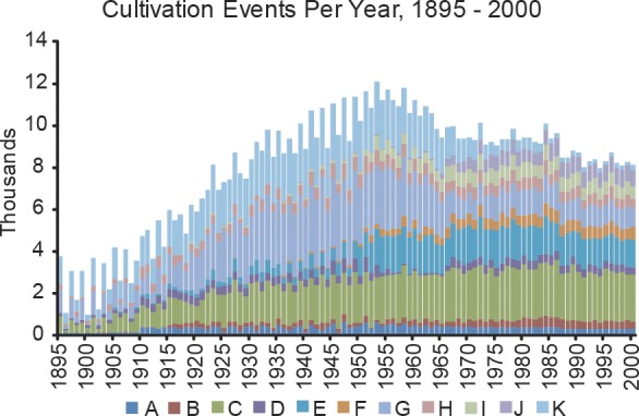
Graph showing the annual number of cultivation events of each type represented in the Daycent simulations, summed over all counties, for 1895–2000.
Fig. S5.

Graph showing the number of horses and tractors on farms in the Great Plains at each USDA Census of Agriculture, 1870–2007.
Irrigation Pumping.
GHG emissions resulting from irrigation in the Great Plains were determined by combining survey, energy cost, and GHG emissions data. The National Agricultural Statistics Service’s 2008 Farm and Ranch Irrigation Survey for South Dakota, Nebraska, Kansas, Colorado, Oklahoma, and Texas (50) provided state-level statistics on the total land area and associated expenses of irrigation with each of the five major energy sources: electricity, natural gas, diesel, liquid petroleum gas/propane/butane, and gasoline/gasohol. State-specific energy price estimates were obtained from the Energy Information Administration (51–55). Irrigation expense and energy price data were combined to derive the total consumption of each energy source by state. GHG emissions per hectare were then obtained for each energy source by combining the GHG intensity of liquid and gas fuels (63) and electricity (64) with the global warming potential (62) of CO2, N2O, and CH4 and dividing total emissions by the total hectares irrigated. A weighted average of the five energy sources was used to arrive at the final emission levels for each state (Table S3).
Table S3.
Annual state-level emission factors for irrigated land
| State | Kilograms of CO2-Ce per hectare |
| Colorado | 314.79 |
| Kansas | 419.04 |
| Nebraska | 206.98 |
| Oklahoma | 391.82 |
| South Dakota | 83.97 |
| Texas | 460.99 |
The South Dakota emission factor was applied to North Dakota, Iowa, and Minnesota, and the Colorado emission factor was applied to Montana, New Mexico, and Wyoming. For the eastern states (Iowa, Kansas, Minnesota, Nebraska, North Dakota, Oklahoma, South Dakota, and Texas), it was assumed that fuel use per unit of irrigated land has been constant since 1930. In the western states (Colorado, Montana, New Mexico, and Wyoming), it was assumed that all irrigation was stream-fed (using no energy) through 1930 and that pump use increased linearly, reaching current proportions (as reflected in the calculated emission factors) in 1950. Emission factors were adjusted accordingly and then applied to the amount of land under irrigation in each county in each year, as specified by the schedule files, and aggregated across the region.
N Fertilizer Production.
Fuel used to produce N fertilizer was calculated annually by weighting the annual amount of N (grams of N per square meter) applied to crops in each schedule file according to the amount of land represented by each file (square meters), aggregating over the region, and converting to grams of CO2-Ce by multiplying by emission factors for N fertilizer production.
Emission factors for N fertilizer production [grams of CO2-Ce (grams of N fertilizer)−1] were computed by taking into account the types of fertilizers used in the US Great Plains from 1960 to 2005 (www.aapfco.org/publications.html; refs. 56–58), the GWI for direct emissions associated with producing N fertilizer material (57, 58), and the energy consumption trends in world NH3 plants, measured in gigajoules per tonne of ammonia [GJ (tonne NH3)−1], from 1955 to 2005 (59). The energy associated with producing NH3 in world plants was ∼62 GJ (tonne of NH3)−1 in 1955, decreasing nonlinearly to 28 GJ (tonne of NH3)−1 in 2005 (59). We calculated energy efficiency ratios for NH3 production by dividing annual energy consumption in world NH3 plants from 1955 to 2005 by the value for 2005 [GJ (tonne of NH3)−1]. The maximum ratio was 2.2 before 1955, decreasing nonlinearly to 1.0 in 2005 (Fig. S6A).
Fig. S6.

Graph showing NH3 production energy efficiency ratio (GJ [tonne of NH3]−1 for the year)/(GJ [tonne of NH3]−1 for 2005) (A), fraction of total Great Plains N fertilizer by fertilizer type (B), and emission factors from fertilizer production [kgCO2-Ce (kg N)−1] (C) from 1950–2005. AmmNit, ammonium nitrate; solns, solutions.
The GWIs for anhydrous/aqueous NH3, urea, N solutions, and ammonium nitrate fertilizers are 0.70, 0.90, 1.59, and 2.33 kg of CO2-Ce (kg of N)−1, respectively (57, 58). The time series of fertilizer use in the United States since 1960 shows an increase in the use of urea and N solutions relative to anhydrous/aqueous NH3 and ammonium nitrate (Fig. S6B). The percentage of total Great Plains N fertilizer that was ammonium nitrate decreased from about 31% in 1960 to 2% in 2005, whereas N solutions increased from 19 to 45% and urea increased from 3 to 28% during the same time period (www.aapfco.org/publications.html; refs. 56–58) (Fig. S6B).
The emission factors for N fertilizer production changed annually from 1955 to 2005 according to the following equation:
| [S4] |
where EFyr is the emission factors for N fertilizer production in year yr [kilograms of CO2-Ce (kilograms of N)−1], EffRatioyr is the energy efficiency ratio of NH3 production relative to the year 2005, GWIi is the GWI for fertilizer type i in year 2005, and fraci,yr is a fraction of total N fertilizer that was fertilizer type i in that year. The resulting emission factors were 3.04 kg of CO2-Ce (kg of N)−1 before 1955, decreasing to 1.22 kg of CO2-Ce (kg of N)−1 in 2005 (Fig. S6C). The decrease in the magnitude of the emission factors related to fertilizer production resulted from the increase in energy efficiency and the decreased use of the fertilizers, such as ammonium nitrate, that have the highest GWIs.
Livestock.
CH4 produced by livestock, through both enteric fermentation and manure management, was calculated using Intergovernmental Panel on Climate Change (IPCC) tier 1 emission factors for dairy and nondairy cattle, horses, mules, pigs, sheep, and chickens (60). Nondairy cattle now produce less enteric CH4 than they did before the spread of feedlots. The emission factor for Oceania (60 kg of CH4 per head−1⋅y−1) was therefore used for enteric CH4 in the period before 1950, because current livestock raising practices in Oceania are similar to livestock raising practices used in the United States earlier in the century. This factor was decreased linearly to the North America emission factor (53 kg of CH4 per head−1⋅y−1) between 1950 and 1970, with the North America factor used in all years since 1970. The North America factor was used for enteric CH4 in all years for dairy cattle; for all other animals, the factor for developed countries was used. North American factors for the management of CH4 emissions from manure were used for cattle and pigs, whereas factors for developed countries were used for all other animals. These factors increased proportionately with mean annual temperature, which was derived for each county from the historic climate data.
Appropriate emission factors for each animal in each county in each year were then applied to annual estimates of the animal population in each county using the US censuses of agriculture for 1880–2007 and interpolating linearly between censuses (3). Data for 1940 and 1950 were excluded because livestock were undercounted in those years (animals born in the calendar year were omitted). County-level totals were aggregated across the region, and kilograms of CH4 were converted to grams of CO2-Ce (Eq. S3).
Estimating the Effects of GHG Abatement Practices, 1990–2000.
Research on alternative agricultural practices has identified modifications that could reduce the GHG fluxes documented in this paper, yet some of these changes come with high costs. For example, the use of slow-release N fertilizer and nitrification inhibitors has the potential to reduce soil N2O fluxes by 14–58% for irrigated and dryland agricultural systems (26). However, farmers currently do not use these improved fertilizers because they typically cost 10–30% more than traditional N fertilizer. New inoculation techniques for cattle can result in a 20–40% reduction in CH4 production (7), but the cost of using the new technology would increase the expense of raising cattle by 20%. Research has also shown that, primarily during the first 10–20 y of adoption, no-tillage cultivation practices (not simulated in our main results) can produce additional storage of 7.0–20.0 g of C per m−2⋅y−1 for dryland systems (27, 28). Irrigated corn rotations in northern Colorado under no-tillage sequestered an additional 15–45 g of C per m−2⋅y−1 in the 0- to 15-cm layer (29) and 65.8–83.9 g of C per m−2⋅y−1 in the 0- to 7.5-cm layer (30). These C sequestration rates for no-tillage cropping in the Great Plains are close to the global potential rate (30 g of C per m−2⋅y−1) derived from multiple reviews (33). The adoption of no-tillage farm practices reduces the amount of energy consumed by farm equipment while increasing both soil water storage and yields in dryland wheat systems. State-level data for the Great Plains indicate that only 14% of land planted in wheat, the dominant crop, used no-tillage practices during 2008 (31).
The impact of using these best-management practices on GHG fluxes in the Great Plains from 1990 to 2000 was evaluated by modeling the effects of the following assumptions:
-
i)
No-tillage practices will result in an average additional C storage of 50.0 g of C per m−2⋅y−1 for irrigated agriculture and 10.0 g of C per m−2⋅y−1 for dryland cropping.
-
ii)
Use of no-tillage practices eliminates fuel use for cultivation of this land but not for planting or harvesting.
-
iii)
Improved fertilizer techniques will result in a net reduction of 30% in N2O emissions in these areas.
-
iv)
CH4 reduction technology will result in a 30% reduction in the production of CH4 by cattle.
These assumptions were used to adjust estimates of soil C storage, soil N2O emissions, and CH4 production from cattle for every year from 1990 to 1999; total GHG fluxes for the decade were then recalculated from these adjusted estimates. We calculated reductions in GHG fluxes using different assumptions about the percentage of farmers who will use the improved practices, ranging from 25% to 100% (25%, 50%, 75%, and 100%). Table 2 shows the impact of different farmer participation rates (25–100%) on soil C fluxes, soil N2O emissions, and net GHG fluxes for dryland and irrigated farming, and the reductions in GHG fluxes associated with tractor fuel use and livestock CH4 fluxes. As expected, the results show an increase in the reductions of GHG fluxes with an increase in the percentage of farmers who use the improved practices. The largest absolute reductions come from the soil C storage (larger negative fluxes) associated with the use of no-tillage cultivation (20–81% reduction). The use of advanced techniques for mitigation of CH4 fluxes from cattle production resulted in an 8–34% reduction, whereas the use of improved fertilizers reduced GHG fluxes by 5–21%.
Table 2.
Summary of mitigation best practices
| Scenario | System before improvements | Reduction from no-till | Improved fertilizer | Improved livestock feed | Total change | System total with improvements |
| Absolute value (and percent change) due to mitigation strategies | ||||||
| Current practices | 102,177 | 102,177 | ||||
| 25% use best practices | 102,177 (0%) | −20,788 (−20%) | −5,401 (−5%) | −8,604 (−8%) | −34,794 (−34%) | 67,383 |
| 50% use best practices | 102,177 (0%) | −41,576 (−41%) | −10,803 (−11%) | −17,208 (−17%) | −69,587 (−68%) | 32,590 |
| 75% use best practices | 102,177 (0%) | −62,364 (−61%) | −16,204 (−16%) | −25,812 (−25%) | −104,381 (−102%) | −2,204 |
| 100% use best practices | 102,177 (0%) | −83,153 (−81%) | −21,606 (−21%) | −34,416 (−34%) | −139,174 (−136%) | −36,997 |
Correlation of System C to Climatic Variables.
Results for the pasture runs demonstrate that, even in the absence of cropping, system GHG fluxes are highly correlated with weather patterns. Fig. S7 charts mean growing season (April–September) maximum daily air temperature and mean cumulative growing season precipitation for the Great Plains from 1895 to 2003 (annual unweighted average across 476 counties). For precipitation, the figure indicates large year-to-year changes (e.g., from 260 mm in 1931 to 373 mm in 1932) and substantial periods of time with above-normal and below-normal precipitation (the mean over the whole period is 373 mm; precipitation was at or below this mean from 1929 through 1940 and above this mean from 1991 to 1997, with the exception of 1994). The figure also illustrates the strong negative correlation between precipitation and temperature: Hotter periods are associated with low precipitation, and cooler periods are associated with above-normal precipitation. The Pearson product-moment correlation coefficient (Pearson’s r) between precipitation and temperature is −0.62, significant at P < 0.0001 (here and in the following statistical tests, n = 51,884 and there were 109 annual observations for each of 476 counties; tests are two-tailed with α = 0.05). Throughout the dry 1930s, maximum temperatures were above the long-term mean of 26.1 °C, yet temperatures were below this mean during the wet period from 1992 through 1997, again with the exception of 1994. The negative correlation between precipitation and temperature is consistent with the idea that dry periods are associated with low cloud cover, higher solar radiation levels, and higher maximum air temperatures. This strong correlation and the large year-to-year changes in mean growing season Great Plains precipitation suggest that the large-scale weather patterns that control precipitation are similar for many of the counties in the Great Plains.
Fig. S7.

Graph showing the time series of cumulative growing season (April–September) precipitation and mean growing season daily maximum air temperature from 1895–2000 (A) and interannual changes in total system C (from Daycent model runs) (B), averaged over the 476 Great Plains counties.
Fig. S7 charts yearly changes in mean Great Plains system C levels along with precipitation. In contrast to the GHG calculations described in the main text, the value of system C shown in Fig. S7 and in the reported correlations and regression was computed as system C in the current year minus system C in the previous year; a positive value represents a gain in system C (sequestration), whereas a negative value represents a loss of C to the atmosphere. We find a positive correlation (Pearson’s r = 0.64, P < 0.0001) between precipitation and C storage, with the system absorbing C in wet years and releasing C in dry years. As expected, given the negative correlation between precipitation and maximum temperature, interannual increases in Great Plains system C levels are also negatively correlated with growing season maximum temperature (Pearson’s r = −0.51, P < 0.0001). Ordinary least squares regression analysis suggests that the best model for C flux would include both temperature and precipitation (R2 = 0.43), and indicates an additional release of 2.71 g of C per square meter for every additional degree in maximum temperature (P = 0.05) and an additional storage of 0.1 g of C per square meter for every additional millimeter of precipitation (P < 0.0001). The correlation between precipitation and change in system C level is consistent with observed eddy covariance net C exchange data that show net C uptake during cool and wet years and net C loss during dry and hot years (65, 66). It is important to note that the figures in the main text use the opposite sign notation, with increases in system C being represented as negative numbers, and decreases in system C as positive numbers.
Net GHG Uncertainty Calculations for the US Great Plains.
We calculated uncertainty using the error propagation equations described in the 2006 IPCC guidelines (67). The IPCC (2006) describes the following rules for combining uncertainties under addition and multiplication, where are the mean values of the input variables and uncertainties () are +1 SD and −1 SD expressed as a percentage of the mean.
The definition of uncertainty (U) for the distribution with mean value is
| [S5] |
where is the variance.
For product total, the uncertainty of the product (Utotal) is calculated as
| [S6] |
For sum total, the uncertainty of the sum (Utotal) is calculated as
| [S7] |
For our analysis, annual uncertainty estimates (1860–2003) were first calculated at the county level for the five major categories of GHG emissions: soil, livestock, tractor fuel, irrigation pumping, and fertilizer production. Next, county level estimates were aggregated for each year to compute annual uncertainty estimates for the entire Great Plains region by GHG category. Finally, total annual uncertainty was computed as the uncertainty of the sum of the five categories. With the error propagation method, relative uncertainty decreases as the absolute value of the sum increases; therefore, annual relative uncertainties of GHG fluxes for the entire Great Plains are smaller than at the county level.
The results from the uncertainty analysis for the Great Plains net GHG fluxes (Fig. S8) show that the absolute value of the uncertainty (Fig. S8A) has a general pattern of increasing from 1860 to 2003, with secondary maxima from 1915 to 1935 and from 1941 to 1942. Absolute uncertainty ranges from 239 Gg of CO2-Ce per year in 1871 to 877 Gg of CO2-Ce per year in 1975. Increasing uncertainty after the 1950s is correlated with increases in livestock CH4; soil N2O emissions; and fuel consumed for irrigation, cultivation, and fertilizer production. The high uncertainty from 1915 to 1935 is associated with the high soil C losses resulting from cultivation of the soil and agricultural expansion. The high uncertainty around 1942 is associated with a large gain in system C due to above-average growing season precipitation.
Fig. S8.

Graph showing the absolute value of uncertainty (Gg CO2-Ce yr−1) (A) and the relative uncertainty (%), of total GHG fluxes in the Great Plains (B) from 1870–2000.
The relative annual uncertainty (Fig. S8B) of total GHG fluxes (annual absolute uncertainty divided by annual net GHG flux) ranges from 1% to 206%, with the highest uncertainty associated with low net GHG fluxes (values close to zero) that are related to variations in weather. Clearly, the relative annual uncertainty has much larger year-to-year variations compared with the absolute values of the net GHG fluxes.
The following describes the relative (percent) uncertainty calculations in more detail. The uncertainty percentages used in these calculations are summarized in Table S4.
Table S4.
Percent uncertainties used in the uncertainty calculations
| Quantity | ± Uncertainty, % | Source |
| Area of each schedule file, m2 | 30 | * |
| Interannual change in soil C | 19 | (68) |
| Soil N2O flux | 34 | (69) |
| Soil CH4 flux | 47 | (70) |
| Livestock enteric CH4 | 40 | table 10.10 (60) |
| Livestock manure CH4 | 30 | table 10.14 (60) |
| Head of livestock in each county | 30 | * |
| Tractor fuel emission factors | 30 | * |
| No. of tractor events in each schedule | 30 | * |
| Irrigation emission factors | 30 | * |
| Area of irrigated land in each state, m2 | 30 | * |
| Energy efficiency ratio for fertilizer production | 30 | * |
| GWIs for fertilizer production | 30 | * |
| Fraction of each fertilizer type used in the Great Plains | 30 | * |
| Amount of fertilizer applied in each schedule | 30 | * |
Where uncertainty was unknown, we assumed it was ±30%.
Biogenic GHGs from soils.
For each schedule file in each county.
For each county, sum net GHG and calculate uncertainty across all schedule files (nschedules).
Soil emissions and uncertainty for the entire Great Plains region (476 counties).
GHG emissions from livestock.
For each livestock category (dairy cattle, nondairy cattle, horses, mules, pigs, sheep, and chickens).
For each county, sum CH4 and calculate uncertainty for all seven livestock categories.
Livestock enteric CH4 emissions for the county:
Livestock manure CH4 emissions for the county:
Total livestock CH4 emissions for the county:
Livestock emissions and uncertainty for the entire Great Plains region (476 counties).
GHG emissions from tractor fuel burning.
For each tractor event (planting, harvesting, and various types of cultivation).
For each schedule file in each county, sum net GHG and calculate uncertainties over all tractor events (nevents).
For each county, sum net GHG and calculate uncertainty across all schedule files (nschedules).
GHG emissions and uncertainty from tractor fuel burning for the entire Great Plains region (476 counties).
GHG emissions from irrigation pumping.
For each state in the Great Plains region.
GHG emissions and uncertainty from irrigation pumping for the entire Great Plains region (12 states).
GHG emissions from fertilizer production.
Emission factor for fertilizer production.
The uncertainty for the emission factor for fertilizer production (UEFyr) is calculated as
where EFyr is the emission factor for N fertilizer production in year, yr [kilograms of CO2-Ce (kilograms of N)−1] (Eq. S4), GWIi is the GWI for fertilizer type i in year 2005, and fraci,yr is fraction of total N fertilizer that was fertilizer type i in that year. The percentage of uncertainty for each quantity was assumed to be 30% (Table S4).
GHG flux and uncertainty for fertilizer in each schedule file.
Assume 30% uncertainty for fertilizer per square meter and 30% uncertainty for area in each schedule:
For each county, sum net GHG and calculate uncertainty across all schedule files (nschedules).
GHG emissions and uncertainty from fertilizer production for the entire Great Plains region (476 counties).
All sources of GHGs in the Great Plains region.
Great Plains Agricultural Land Use History
Land use in the Great Plains region has changed dramatically over the past 150 y, and can be divided into three sequential regimes (Fig. 2). Grazing dominated during the first regime, with cattle succeeding bison after the US Civil War. The second regime began in the 1870s, with crop-based agriculture introduced first in the eastern plains and then moving westward through the 1930s. The third regime dates from the mid-1930s and is characterized by the rapid adoption of such new agricultural technologies as (i) mechanical cultivation equipment, (ii) inorganic fertilizers, (iii) pump irrigation, and (iv) new high-yielding crop varieties bred for synergy with other new inputs (22–24). This period has also seen a substantial increase in beef cattle production in the Great Plains, both in absolute numbers and as a proportion of all livestock, especially from the 1940s to the 1960s (Fig. 2D).
Fig. 2.

Changing agricultural practices in the US Great Plains, 1870–2000. (A) Transition from native pasture (Pasture) to dryland cropland (Dryland) in the first half of the 20th century, followed by an increase in irrigated cropland (Irrigated) and the restoration of previously cropped land (Out of Production) (20). (B) Total plant production of three major crops (corn, wheat, and hay) (6). (C) Amount of N fertilizer applied to dryland cropland (Dryland), the amount applied to irrigated cropland (Irrigated), and the total of the two (Total) (6). (D) Livestock populations expressed as animal units (nondairy cattle = 1, dairy cattle = 1.4, horse = 1, mule = 1, pig = 0.4, sheep = 0.1, chicken = 0.033) (20, 21).
The dominant crops in the northern and central Great Plains are winter wheat, spring wheat, and corn. Winter wheat, sorghum, corn, and cotton are the most prevalent crops in the south (23). Dryland cropping predominates, except along the major river systems and over the Ogallala aquifer, where irrigation water is available. The amount of irrigated agricultural land increased substantially in the 1950s, and then stabilized by the 1980s, with over 15 million acres irrigated with pumped water (Fig. 2A). Land was increasingly retired from crop production beginning in the 1950s, largely through enrollment in federally sponsored conservation programs. An analysis of the most recent US Census of Agriculture (through 2012) suggests that about 20% of the 1950s dryland cropping area is no longer used for that purpose, with about half of that change a result of increased irrigated cropping and about half a result of a long-term reduction in cropland. The data also show a 31% decrease in land in the Conservation Reserve Program (CRP) between its maximum in 2007 and 2012. We suspect that improved corn prices have led farmers to convert CRP land into cropland. The consequence of plowing out CRP land would be to release C from the soil and increase N2O emissions (25).
Total production for all crops was low before 1940. Production rose thereafter as farmers experienced rapid increases in corn, hay, cotton, and wheat yields from the 1940s to the 1970s; corn yields have continued to grow since then (Fig. 2B). Parton et al. (6) attribute the larger crop yields to the increased use of fertilizer (Fig. 2C), new crop varieties (22), improved soil tillage practices for wheat, use of herbicides and insecticides, and the expansion of irrigation, all of which generates a yield increment of 100–300% in cotton, hay, and corn production.
Patterns of livestock raising have also changed over the past 150 y. The number of domestic animals rapidly increased from 1870 to 1900 (Fig. 2D), by which time more than 12 million beef cattle had replaced the bison herds on the Great Plains. After a period of stability from 1900 to 1935, the number of beef cattle increased by 120% from 1935 to 1970, whereas the number of horses and dairy cattle declined due to the substitution of mechanical power for horse power in agriculture and the concentration of dairies in other parts of the country. Many of these cattle reside in feedlots, a major consumer of the increasing quantities of corn and hay produced under irrigation.
Although many of the changes in agricultural practices just described were accomplished by the 1970s, change has continued, and efforts to improve agricultural productivity and efficiency are reflected in the results reported here. The previously unidentified estimates stated in this article were made using the best available data and methods. As farmers and scientists look to the future, many emerging agricultural best practices show promise for continued productivity coupled with reduced environmental consequences. The implementation of these best-management practices offers the potential for reducing GHG fluxes from Great Plains agricultural systems. Examples of these practices are well known and well documented, and include (i) use of slow-release N fertilizer and nitrification inhibitors with the potential to reduce soil N2O fluxes by 14–58% for irrigated and dryland agricultural systems (26), (ii) use of no-tillage cultivation practices that can produce a net C storage of 7.0–20.0 g of C per m−2⋅y−1 for dryland systems (27, 28) and 15.0–83.9 g of C per m−2⋅y−1 for irrigated systems (29, 30), and (iii) use of new inoculation techniques for cattle that can result in a 20–40% reduction in CH4 production (7). The adoption of no-tillage farm practices would also reduce the amount of energy consumed by farm equipment and increase both soil water storage and yields in dryland wheat systems. Currently, no-tillage cultivation is used by fewer than 15% of wheat farmers (the dominant crop) in the Great Plains (31). Recent papers suggest the previous estimates of soil C storage under no-till agriculture have been overestimated (32, 33) because most of the soil C measurements did not consider the changes to soil C below the plow zone (0- to 20-cm layer). In contrast to that finding, a recent review paper supports the results from earlier studies that show substantial increases in soil C under no-tillage cultivation for dry agricultural regions similar to the Great Plains (34, 35).
Results
GHG Fluxes by Land Use Category.
Estimates of GHG fluxes related to cropping are combined from separate analyses of four agricultural land use systems (dryland cropping, irrigated cropping, land removed from crop production, and pasture land). Fig. 3 shows GHG emissions annually by land use category, with separate results for system C [positive when lost (released) and negative when sequestered (stored)], soil N2O emissions (always positive), and CH4 absorbed by the soil (always negative). The GHG fluxes for N2O and CH4 are shown as CO2-Ce fluxes using standard corrections needed to account for the differential GHG warming potentials of N2O and CH4 (N2O is 298-fold more effective than CO2, and CH4 is 25-fold more effective than CO2). System C includes soil C (>95% of total C) and live and dead plant C pools, with most of the changes in system C resulting from changes in soil C. These results are weighted to reflect the actual amount of land in each use category across the region. Because a relatively small amount of land was used for irrigated cropping or taken out of production (Fig. 3), the scale for Fig. 3 B and C is an order of magnitude smaller than the scale for the panels representing dryland cropping (Fig. 3A) and pasture (never-cropped) land (Fig. 3D).
Fig. 3.

Estimates of GHG fluxes by land use category showing soil N2O emissions (always positive) and CH4 consumption (always negative), and the change in system C since the previous year (either positive or negative), expressed in gigagrams of CO2-Ce (Gg CO2-Ce y−1): dryland cropland (A), irrigated cropland (B), dryland cropland restored to grassland (C), and native pasture (D). Positive values indicate GHG sources into the atmosphere, whereas negative values indicate a terrestrial sink. The solid black line represents the 9-y moving average of the total GHG flux (sum of soil N2O, CH4, and system C change). The red solid line represents the 9-y moving average of the change in total system C.
Simulated soil GHG fluxes from dryland cropping in the Great Plains (Fig. 3A) show a steady increase in system C loss (primarily from the soil C pool) and N2O fluxes from 1900 to 1930, a result of the progressive plow-out of native prairie grasslands that culminated in most parts of the region during the 1930s. System C losses slowed after the 1930s, partly as a result of the stabilization of the amount of land in crop production and partly because the loss of soil C from cultivation markedly diminished after the first 20 y of cultivation (36). A general pattern of low-level system C sequestration began in the 1960s, resulting from a reduction in the number and intensity of soil tillage events. At the same time, however, soil N2O fluxes increased by as much as 100% due to an increase in the use of N fertilizer (Fig. 2C).
Model results for irrigated cropping systems in the Great Plains (Fig. 3B) show low levels of system C loss before the 1950s because relatively few counties irrigated before that time. Irrigated agriculture was initiated after 1950 in most areas where land had already been plowed for dryland cultivation, and thereby depleted of soil C. As irrigation became more widespread on former dryland cropping areas between the 1950s and the 1970s, both system C storage (removing GHGs from the atmosphere) and soil N2O fluxes (releasing GHGs into the atmosphere) increased dramatically (6). These increases reflect the enhancement of plant production and C inputs to the soil associated with irrigation (6, 37), as well as the expansion of irrigated land (Fig. 2A). System C storage peaked in the 1970s and then decreased as the soil C storage potential of the irrigated soils was reached. Soil N2O fluxes increased in tandem with N fertilizer application beginning in the 1950s (Fig. 2C). Irrigated cropping represents a net sink of GHGs from 1950 through the 1980s, with fluxes reaching their lowest negative values in the 1970s and then turning positive by the 1990s as the soil saturated with C and N2O fluxes continued to increase.
Simulations of the abandonment of dryland cropping (out of production; Fig. 3C) show a dramatic increase in system C storage, resulting from the accumulation of soil C with the cessation of cropping and tillage (38–40). Increases in C storage over time reflect both the restoration of grassland (perennial grasses have more root growth than annual crops) and increases in the amount of land taken out of production, particularly during the 1960s and then again with the implementation of the CRP in the 1980s (41). Restoration of native soil fertility takes 100 y or more unless fertilizer is added to the system. However, even the slow accumulation of C more than offsets soil N2O fluxes, which remain low in the restored grassland because of low soil fertility. Net GHG fluxes in this system are therefore negative throughout the period.
Modeled GHG fluxes for pasture (Fig. 3D) are neutral on the whole, with positive GHG emissions from soil N2O balanced by negative fluxes from CH4 uptake by the soil. System C fluxes vary substantially from year to year with precipitation, showing a general pattern of net C losses during dry years and net C gains during wet years. Growing season precipitation is negatively correlated with growing season maximum air temperature (42, 43). System C storage is positively correlated with growing season precipitation and negatively correlated with growing season maximum air temperature; thus, pasture system C levels increase (C sequestration − negative fluxes) during cold and wet summers and decrease (C release − positive fluxes) during hot and dry summers. This pattern is clearly demonstrated by C losses during the dry 1930s and C uptake during the wet 1990s. Details can be found in SI Materials and Methods.
All Sources of GHG Emissions.
Fig. 4A summarizes the results from Fig. 3. As cropping expanded from the late 19th century into the 20th century, an ever-larger quantity of GHG emissions was released into the atmosphere, peaking in the 1930s at levels as high as 35,000 Gg of CO2-Ce per year. The most prominent source of GHG emissions during this period was the loss of soil C associated with the plowing of native grasslands, a practice that had nearly ended by the early 1930s. Soil C losses diminished rapidly from 1930 into the 1950s, with soil C sequestration starting after the 1960s, as a result of both soil C stabilization in dryland systems and soil C storage in irrigated cropland and restored grasslands (cropland out of production). The cultivation of native grasslands also produced a pattern of increasing soil N2O fluxes beginning in 1900. N2O emissions rose by another 30% between 1940 and 2000 due to increased fertilizer application in irrigated and dryland cropping systems. After 1970, C sequestration in restored grasslands and irrigated cropland offset N2O emissions and produced net negative GHG fluxes in the system as a whole. This pattern of GHG sequestration was enhanced in the 1990s when above-average rainfall increased C storage in native prairie and restored grasslands.
Fig. 4.

GHG fluxes from 1870 to 2000 (Gg CO2-Ce y−1). (A) Total emissions from the four land use categories in Fig. 3 (Dryland Cropland, Irrigated Cropland, Out of Production Land, and Native Pasture). (B) Tractor fuel use for planting, harvesting, and cultivation (Tractor Fuel); fuel use for irrigation pumping (Irrigation Fuel); and GHG emissions from fertilizer production (Fertilizer Production). (C) Livestock enteric CH4 and manure CH4 emissions. (D) GHG fluxes from all agricultural sources, including livestock enteric CH4 and manure CH4 emissions (Livestock CH4, brown bars); fuel used for tractors, irrigation pumping, and fertilizer production (Fuel & Fertilizer, pink bars); soil N2O, CH4, and system C change from the four land use categories [Ecosystem GHG Flux, solid light green line], representing the 9-y moving average of the change in the soil/plant system GHG fluxes (sum of soil N2O, CH4, and system C change); and the sum of all sources (Total System GHG Flux, solid black line), representing the 9-y moving average of the total GHG flux from soil/plant, tractor fuel, irrigation pumping, fertilizer manufacture, and livestock production.
Since the 1930s, farmers have increased plant productivity by (i) using gasoline and diesel equipment to cultivate, plant, and harvest their lands; (ii) applying synthetic fertilizer to raise crop productivity; and (iii) irrigating fields to ensure sufficient moisture for plant growth. GHG fluxes from tractor fuel peaked in the 1950s and then declined, with most energy used throughout the period for cultivation rather than planting or harvesting (Fig. 4B). The decline since the 1950s is largely due to less intensive cultivation and a shift from gasoline to more energy-efficient diesel engines. The scale of GHG fluxes from equipment is relatively small, with the peak just over 3,500 Gg of CO2-Ce per year, compared with peaks from the soil systems 10-fold as high in the 1930s (Fig. 4A). GHG fluxes from energy used for fertilizer production and irrigation pumping increased steadily after onset of use in the 1940s (Fig. 4B). Fluxes from irrigation pumping have remained constant since the 1970s, as the amount of irrigated land has stabilized and pumps have shifted from gasoline to electric power. At the same time, GHG emissions associated with fertilizer production increased rapidly from virtually nothing in the 1930s and 1940s to a peak in the late 1960s of nearly 4,700 Gg of CO2-Ce per year, followed by a slow decline to about 3,500 Gg of CO2-Ce per year in the late 1990s.
The last element in our comprehensive estimate of GHG emissions from Great Plains agriculture is the CH4 produced by the livestock sector. Overall, livestock numbers increased slowly but steadily in the area during the 20th century (Fig. 2D). The use of horses for maintaining agricultural lands decreased as tractors were adopted. In addition, the number of dairy cattle decreased as other regions of the United States began to specialize in dairy production. Nondairy cattle were quickly substituted, becoming consumers of the region’s increasing corn production. As generators of enteric and manure CH4, livestock are large and growing contributors to regional GHG fluxes (Fig. 4C).
Fig. 4D combines all of the elements discussed above into previously unidentified estimates of annual net GHG emissions from US Great Plains agriculture between 1870 and 2000 (presented numerically in Table 1). Early exploitation of the soil by agriculture (from the late 19th century until the 1930s) produced a net positive GHG flux, peaking in the particularly dry 1930s at an average rate of 45,000 Gg of CO2-Ce per year. After that time, contributions from soil systems diminished, whereas contributions from livestock increased, reaching 12,000 Gg of CO2-Ce per year in the 1990s, due to extensive use of the region for cattle feeding. By the 1950s, fuel consumed for irrigation, mechanized cultivation, and fertilizer production had also become an important source of net GHG emissions, at about 7,000 Gg of CO2-Ce per year by the end of the century. Total GHG fluxes have decreased since the period of soil plow-out (they are now close to 12,000 Gg of CO2-Ce per year) but are nonetheless steady and positive.
Table 1.
Net GHG fluxes from all sources (gigagrams of CO2-Ce): Annual average by decade
| Decade | Pasture | Dryland | Irrigated | Out of production | Tractor | Irrigation | Fertilizer | Livestock | Total |
| 1870 | −1,491 | 441 | 0 | 0 | 0 | 0 | 0 | 824 | −225 |
| 1880 | 4,121 | 8,266 | 28 | 0 | 0 | 0 | 0 | 2,967 | 15,382 |
| 1890 | 1,624 | 13,328 | 94 | 0 | 0 | 0 | 0 | 6,378 | 21,423 |
| 1900 | −4,154 | 15,597 | 109 | 0 | 0 | 0 | 0 | 8,318 | 19,871 |
| 1910 | 1,651 | 22,027 | 83 | 0 | 0 | 0 | 1 | 9,205 | 32,967 |
| 1920 | −1,173 | 31,230 | 392 | 0 | 383 | 0 | 7 | 9,914 | 40,715 |
| 1930 | 4,636 | 25,359 | 194 | 0 | 1,410 | 127 | 18 | 9,811 | 41,398 |
| 1940 | −4,453 | 18,283 | 220 | 0 | 2,503 | 455 | 55 | 10,749 | 27,516 |
| 1950 | 376 | 9,900 | −306 | −352 | 3,162 | 1,101 | 2,527 | 10,645 | 26,630 |
| 1960 | −301 | 2,969 | −872 | −2,457 | 2,571 | 1,659 | 3,960 | 11,153 | 18,341 |
| 1970 | −945 | −937 | −1,017 | −1,910 | 1,944 | 2,018 | 3,868 | 11,800 | 14,475 |
| 1980 | −735 | 1,030 | −392 | −2,200 | 1,697 | 1,811 | 3,660 | 11,553 | 16,108 |
| 1990 | −4,109 | −2,311 | 293 | −2,919 | 1,574 | 1,890 | 3,500 | 12,300 | 9,929 |
The uncertainty in these results is presented in SI Materials and Methods, which shows that the absolute value of the uncertainty generally increases from 1860 to 2003, with secondary uncertainty maxima from 1915 to 1935. Absolute uncertainty ranges from 239 Gg of CO2-Ce per year in 1871 to 877 Gg of CO2-Ce per year in 1975. Increasing absolute uncertainty after the 1950s is correlated with increases in livestock CH4; soil N2O emissions; and fuel consumed for irrigation, cultivation, and fertilizer production. The high uncertainty in GHG fluxes from 1915 to 1935 is associated with the high soil C losses resulting from cultivation of the soil and expansion of agriculture. The relative annual uncertainty of total GHG fluxes (annual absolute uncertainty divided by observed annual net GHG flux) ranges from 1 to 206%, with the highest relative uncertainty associated with low net GHG fluxes (values close to zero).
GHG Reductions Using Best-Management Practices.
The combined impact of best-management practices for Great Plains farming in the 1990s (current GHG fluxes from farming) was determined by (i) assuming that no-tillage practices would lead to an additional storage of 50 g of C per m−2⋅y−1 in irrigated cropping (29, 30) and an additional storage of 10.0 g of C per m−2⋅y−1 in dryland cropping (27, 28), (ii) a 30% reduction in soil N2O fluxes by using improved fertilizer techniques (26), and (iii) a 30% reduction in CH4 (7) due to improved cattle management (the method of estimation is provided in SI Materials and Methods). Due to the uncertainty of farmer adoption rates, we made our assessments assuming a range of 25%, 50%, 75%, and 100% (44). Results (Table 2) show a 34% reduction in net GHG fluxes, with 25% of farmers adopting the new methods. Most of the reduction (60%) resulted from the use of no-tillage cultivation practices, 25% resulted from the CH4 mitigation from cattle, and 15% resulted from the use of improved fertilizer. A 75% increase in farmer adoption rates resulted in a 102% reduction, whereas a 100% rate increase resulted in a 136% reduction (C sequestration).
Discussion
The results of this research reveal a complex picture, which is neither optimistic nor pessimistic, regarding agriculture’s contribution to net GHG emissions, especially if we look to the future. If we begin with the historical account of estimated emissions from land management (Fig. 4A), the conclusion may be encouraging, suggesting that after a century of soil exploitation through cropping, the agricultural systems of the Great Plains had begun to stabilize by the 1970s, with relatively modest emissions of GHGs and the potential for C sequestration to offset soil N2O emissions. However, Table 1 shows that conclusion to be inappropriate. Even if cropping systems have sequestered some C since the 1960s, all other parts of the agricultural system (including those parts that facilitated C sequestration) continue to produce net positive GHG fluxes, with the largest contributions coming from livestock production and smaller, yet nontrivial, amounts coming from equipment use, fertilizer, and irrigation. Although there is uncertainty in these estimates, that uncertainty is small compared with the historical changes in GHG fluxes over 130 y. The historical patterns described here show the important roles played by the series of technological transformations that have swept over agriculture since 1870. The patterns themselves partly reflect public policies that have altered where and how these lands have been used for agriculture. Within this human-dominated system, however, it is critical to notice the fundamental influence of climatic variation, which is apparent in Daycent model results for never-cropped land (pasture; Fig. 3D). Independent of technological change and policy impacts, when precipitation was high and temperature was low, C was stored. Conversely, when temperature was high and precipitation was low, C was released. Interannual changes in system C on pasture land ranged from a storage of 41 g of C per square meter in the wet year of 1942 to a release of 27 g of C per square meter in the dry year of 1934. Table 1 indicates that in the 1990s, fuel (tractor and irrigation), fertilizer, and livestock in the Great Plains produced 19,263 Gg of CO2-Ce of GHG emissions (Fig. 4D). Because it was a particularly wet decade, 21% of this release was absorbed by the pasture system, but results for pasture in the dry 1930s suggest that the pasture system could also increase the release of GHG emissions by the same percentage under less favorable weather conditions. Climatic changes, therefore, have the potential to alter yearly net GHG fluxes greatly.
Our results suggest that use of best agricultural management practices has the potential to reduce net GHG fluxes from the Great Plains agricultural system greatly, depending on the rate of adoption by farmers (a 34–136% reduction as rates of adoption increased from 25–100%). Most of the reduction (60%) resulted from the use of no-tillage cultivation practices, 25% resulted from the CH4 mitigation from cattle, and 15% resulted from the use of improved fertilizer. The use of no-tillage cultivation has increased over the past 10 y (44), and has the potential to reduce GHG fluxes for the Great Plains greatly, because only 14% of land planted in wheat, the dominant crop, used no-tillage practices during 2008 (31). The reduction in GHG fluxes from C sequestration due to the use of no-tillage practices primarily occurs during the first 20 y following initiation of the practice; however, the GHG reductions from the use of CH4 mitigation from cattle and improved fertilizer result in permanent annual reductions. These reductions from the Great Plains agricultural system could potentially contribute to the goal of the Obama administration to reduce GHG fluxes from agricultural systems in the United States by more than 25% during the next 10 y (45, 46). The technologies to implement these best-management practices are currently available; however, farmers will not adopt them unless financial incentives are offered, given the resultant cost increase for raising both crops and livestock.
This research has estimated the overall production of positive net GHG fluxes from Great Plains agriculture at about 2.9 million Gg of CO2-Ce between 1870 and 2000. Although this figure is large, almost 50% of the total emissions are a result of the expansion of dryland agriculture before 1950. Clearly, the major sources of GHG fluxes have evolved over time. Before 1950, most emissions came from soil C losses related to cultivation. Currently, the majority of GHG fluxes result from livestock production and energy used by farm equipment, fertilizer synthesis, and irrigation (Table 1). As a result of these findings, this article suggests that the use of existing best-management practices could greatly reduce GHG emissions from US Great Plains agricultural systems if economic incentives were available to promote their use.
Materials and Methods
The Daycent ecosystem model was used to estimate soil GHG fluxes associated with cropping in each of 476 Great Plains counties (19). The model is driven by county-level weather and soil data (42, 43, 47) and detailed assumptions about daily agricultural management practices. These practices include cultivation, planting, irrigation, fertilizer application, and harvesting over the simulation period, and were derived from historical documents reflecting historical changes in crop varieties, technology, and cropping techniques (37). Each major dryland and irrigated rotation system, as well as unplowed native grassland, was modeled separately, as was land removed from crop production either before or under the CRP. The model was verified and validated with yield data from national agricultural databases (19) (www.nass.usda.gov) and scaled to the county level using historical agricultural census data (20). Daycent output includes interannual change in system C and annual amounts of N2O release and CH4 absorption. GHG flux is calculated by converting each component to CO2-Ce and summing over components. Calculation of the uncertainty in our estimates of GHG fluxes from each component of agriculture and for the total annual agricultural GHG flux in the Great Plains is detailed in SI Materials and Methods.
The assumptions about agricultural management practices that drive the Daycent model also provided estimates of historical amounts of tractor use, irrigation, and fertilizer application in each county over the simulation period. Fuel consumed during tractor use was estimated using the Agricultural Machinery Management Data from the American Society of Agricultural and Biological Engineers Standards (48, 49). Fuel consumed in irrigation pumping was estimated by combining data from the National Agricultural Statistics Service’s 2008 Farm and Ranch Irrigation Survey (50) with energy price data from the Energy Information Administration (51–55). Historical GHG emissions from the production of N fertilizer were calculated by combining the current global warming intensity from production of commercial N fertilizer products with both the historical changes in the type of N fertilizer products used by farmers (www.aapfco.org/publications.html; refs. 56–58) and changes in the efficiency of producing the different types of N fertilizer products (59). CH4 produced by livestock enteric fermentation and manure management was calculated using Intergovernmental Panel on Climate Change tier 1 emission factors for dairy and nondairy cattle, horses, mules, pigs, sheep, and chickens (60). Regional totals for all sources of GHG flux were derived by aggregating county-level estimates. Full details are available in SI Materials and Methods.
At the beginning of our analysis, energy use and GHG fluxes were clearly bounded by the local farm experience. They became less so over time in two ways. First, the energy used in pump-driven irrigation, which was powered by gasoline engines in the 1940s and 1950s and partly converted to diesel later, is now largely powered by electricity. The GHG fluxes involved in electricity generation are now remote from the agricultural enterprise. Second, synthetic fertilizer has been substituted for locally produced manure since the 1950s. We have included both the energy used for irrigation pumping and the energy used to produce synthetic fertilizer in our analysis because to exclude either one at any given point in time would disrupt the long-term aspect of our work, for which irrigation pumping and fertilizer production and use are essential.
Potential reductions in GHG fluxes due to improved agricultural practices were estimated by taking the calculated GHG contributions by agricultural category for the 1990s and reducing them by fixed amounts of C stored for no-tillage cropping practices and by percentages of GHG flux for improved fuel use, fertilizer, and cattle management. Because we do not know the proportion of farmers who might make use of these improved practices, we then estimated the overall and agricultural category impacts on GHG fluxes assuming that 25%, 50%, 75%, and 100% of farmers would do so. A more detailed description of the methods used can be found in SI Materials and Methods.
Acknowledgments
This research was supported by Grant R01HD33554 from the Eunice Kennedy Shriver National Institute of Child Health and Human Development; the Shortgrass Steppe Long-Term Ecological Research Site [National Science Foundation (NSF) Grant DEB-0823405] at Colorado State University; US Department of Agriculture (USDA) cooperative research projects (Grants 58-5402-4-001 and 59-1902-4-00); USDA Ultraviolet-B (Grant 2014-34263-22038); USDA National Institute of Food and Agriculture (Grant 2015-67003-23456); and the Inter-university Consortium for Political and Social Research at the Institute for Social Research, University of Michigan. We thank Cindy Keough for her assistance with the Daycent model, Glenn Deane for statistical consultation, and Laurie Richards for editorial assistance. The National Science Foundation supported some of M.P.G.'s work on this article.
Footnotes
The authors declare no conflict of interest.
This article is a PNAS Direct Submission.
Data deposition: The data reported in this paper have been deposited at the Inter-university Consortium for Political and Social Research (ICPSR) at the University of Michigan. ICPSR 31681: Great Plains Population and the Environment Data: Biogeochemical Modeling Data 1860–2003.
This article contains supporting information online at www.pnas.org/lookup/suppl/doi:10.1073/pnas.1416499112/-/DCSupplemental.
References
- 1.US EPA . Inventory of US Greenhouse Gas Emissions and Sinks: 1990–2005. US Environmental Protection Agency; Washington, DC: 2007. Available at www.epa.gov/climatechange/Downloads/ghgemissions/07CR.pdf. Accessed March 6, 2014. [Google Scholar]
- 2.US Department of Agriculture . United States Census of Agriculture 2007, Volume 1, Chapter 2: County Level Data. USDA, National Agricultural Statistics Service; Washington, DC: 2009. Available at www.agcensus.usda.gov/Publications/2007/Full_Report/Volume_1,_Chapter_2_County_Level/. Accessed August 1, 2011. [Google Scholar]
- 3.Sala OE, Lauenroth WK, Parton WJ, Trlica MJ. Water status of soil and vegetation compartments in the shortgrass steppe. Oecologia. 1981;48(3):327–331. doi: 10.1007/BF00346489. [DOI] [PubMed] [Google Scholar]
- 4.Del Grosso S, et al. Global potential net primary production predicted from vegetation class, precipitation, and temperature. Ecology. 2008;89(8):2117–2126. doi: 10.1890/07-0850.1. [DOI] [PubMed] [Google Scholar]
- 5.Matson PA, Parton WJ, Power AG, Swift MJ. Agricultural intensification and ecosystem properties. Science. 1997;277(5325):504–509. doi: 10.1126/science.277.5325.504. [DOI] [PubMed] [Google Scholar]
- 6.Parton WJ, Gutmann MP, Ojima D. Long-term trends in population, farm income, and crop production in the Great Plains. Bioscience. 2007;57(9):737–747. [Google Scholar]
- 7.Boadi D, Benchaar C, Chiquette J, Masse D. Mitigation strategies to reduce enteric methane emissions from dairy cows: Update review. Can J Anim Sci. 2004;84(3):319–335. [Google Scholar]
- 8.De Jong, et al. Land-use change and carbon flux between 1970s and 1990s in Central Highlands of Chiapas, Mexico. Environ Manage. 1999;23(3):373–385. doi: 10.1007/s002679900193. [DOI] [PubMed] [Google Scholar]
- 9.Flessa H, et al. Integrated evaluation of greenhouse gas emissions (CO2, CH4, N2O) from two farming systems in southern Germany. Agric Ecosyst Environ. 2002;91(1-3):175–189. [Google Scholar]
- 10.Cavigelli MA, et al. US agricultural nitrous oxide emissions: Context, status, and trends. Front Ecol Environ. 2012;10(10):537–546. [Google Scholar]
- 11.Beach RH, et al. 2010. Model Documentation for the Forest and Agricultural Sector Optimization Model with Greenhouse Gases (FASOMGHG). Report for the United States Environmental Protection Agency (Research Triangle Institute International, Research Triangle Park, NC)
- 12.McCarl BA, Schneider UA. Climate change. Greenhouse gas mitigation in U.S. agriculture and forestry. Science. 2001;294(5551):2481–2482. doi: 10.1126/science.1064193. [DOI] [PubMed] [Google Scholar]
- 13.Del Grosso SJ, Mosier AR, Parton WJ, Ojima DS. DAYCENT model analysis of past and contemporary soil N2O and net greenhouse gas flux for major crops in the USA. Soil Tillage Research. 2005;83(1):9–24. [Google Scholar]
- 14.Tian H, et al. Contemporary and projected biogenic fluxes of methane and nitrous oxide in North American terrestrial ecosystems. Front Ecol Environ. 2012;10(10):528–536. [Google Scholar]
- 15.Cole CV, et al. Global estimates of potential mitigation of greenhouse gas emissions by agriculture. Nutrition Cycling in Agroecosystems. 1997;49(1-3):221–228. [Google Scholar]
- 16.Liebig MA, et al. Greenhouse gas contributions and mitigation potential of agricultural practices in northwestern USA and western Canada. Soil Tillage Research. 2005;83(1):25–52. [Google Scholar]
- 17.Johnson JMF, et al. Greenhouse gas contributions and mitigation potential of agriculture in the central USA. Soil Tillage Research. 2005;83(1):73–94. [Google Scholar]
- 18.Robertson GP, Grace PR. Greenhouse gas fluxes in tropical and temperate agriculture: The need for a full-cost accounting of global warming potentials. In: Wassmann R, Vlek PLG, editors. Tropical Agriculture in Transition—Opportunities for Mitigating Greenhouse Gas Emissions? Springer; Dordrecht, The Netherlands: 2004. pp. 51–63. [Google Scholar]
- 19.Hartman MD, et al. Impact of historical land-use changes on greenhouse gas exchange in the U.S. Great Plains, 1883-2003. Ecol Appl. 2011;21(4):1105–1119. doi: 10.1890/10-0036.1. [DOI] [PubMed] [Google Scholar]
- 20.Gutmann M. 2005 Great Plains population and environment data: Agricultural data, 1870–1997 United States (Machine-readable dataset, ICPSR 04254-v1) (University of Michigan, Inter-university Consortium for Political and Social Research, Ann Arbor, MI). Available at dx.doi.org.proxy.lib.umich.edu/10.3886/ICPSR04254. Accessed August 1, 2011.
- 21.Minnesota Department of Agriculture Animal Unit Calculation Worksheet. 2014 Available at www.mda.state.mn.us/animals/feedlots/feedlot-dmt/feedlot-dmt-animal-units.aspx. Accessed August 15, 2011.
- 22.Dalrymple DG. Changes in wheat varieties and yields in the United States, 1919-1984. Agric Hist. 1988;62(4):20–36. [Google Scholar]
- 23.Cunfer G. On the Great Plains: Agriculture and Environment. Texas A&M Univ Press; College Station, TX: 2005. [Google Scholar]
- 24.Olmstead A, Rhode P. Creating Abundance: Biological Innovation and American Agricultural Development. Cambridge Univ Press; New York: 2008. [Google Scholar]
- 25.Follett RF, Varvel GE, Kimble JM, Vogel KP. No-till corn after bromegrass: Effect on soil carbon and soil aggregates. Agron J. 2009;101(2):261–268. [Google Scholar]
- 26.Akiyama H, Yan X, Yagi K. Evaluation of effectiveness of enhanced-efficiency fertilizers as mitigation options for N2O and NO emissions from agricultural soils: Meta-analysis. Glob Change Biol. 2010;16(6):1837–1846. [Google Scholar]
- 27.Conant R, Ogle S, Paul E, Paustian K. Measuring and monitoring soil organic carbon stocks in agricultural lands for climate mitigation. Front Ecol Environ. 2011;9(3):169–173. [Google Scholar]
- 28.Ogle S, Breidt F, Paustian K. Agricultural management impacts on soil organic carbon storage under moist and dry climatic conditions of temperate and tropical regions. Biogeochemistry. 2005;72(1):87–121. [Google Scholar]
- 29.Halvorson AD, Jantalia CP. Nitrogen fertilization effects on irrigated no-till corn production and soil carbon and nitrogen. Agron J. 2011;103(5):1423–1431. [Google Scholar]
- 30.Mosier AR, Halvorson AD, Peterson GA, Robertsone GP, Sherrod L. Measurement of net global warming potential in three agroecosystems. Nutrition Cycling in Agroecosystems. 2005;72(1):67–76. [Google Scholar]
- 31. Conservation Technology Information Center (2015) National Crop Residue Management Survey. Available at www.ctic.org/CRM/. Accessed April 24, 2015.
- 32.Baker JM, Ochsner TE, Venterea RT, Griffis TJ. Tillage and soil carbon sequestration- What do we really know? Agric Ecosyst Environ. 2007;118(1-4):1–5. [Google Scholar]
- 33.Powlson DS, et al. Limited potential of no-till agriculture for climate change mitigation. Nat Clim Change. 2014;4(8):678–683. [Google Scholar]
- 34.Syswerda SP, Corbin AT, Mokma DL, Kravchenko AN, Robertson GP. Agricultural management and soil carbon storage in surface vs. deep layers. Soil Sci Soc Am J. 2011;75(1):92–101. [Google Scholar]
- 35.Angers DA, Eriksen-Hamel NS. Full-inversion tillage and organic carbon distribution in soil profiles: A meta-analysis. Soil Sci Soc Am J. 2008;72(5):1370–1374. [Google Scholar]
- 36.Haas H, Evans C. Nitrogen and Carbon Changes in Great Plains Soils as Influenced by Cropping and Soil Treatments. USDA, Government Printing Office; Washington, DC: 1957. Technical Bulletin 1164. [Google Scholar]
- 37.Parton WJ, Gutmann MP, Williams SA, Easter M, Ojima D. Ecological impact of historical land-use patterns in the Great Plains: A methodological assessment. Ecol Appl. 2005;15(6):1915–1928. [Google Scholar]
- 38.Burke IC, Elliott ET, Cole CV. Influence of macroclimate, landscape position, and management on soil organic matter in agroecosystems. Ecol Appl. 1995;5(1):124–131. [Google Scholar]
- 39.Robles MD, Burke IC. Soil organic matter recovery on Conservation Reserve Program fields in southeastern Wyoming. Soil Sci Soc Am J. 1998;62(3):725–730. [Google Scholar]
- 40.VandenBygaart AJ, et al. Impact of sampling depth on differences in soil carbon stocks in long-term agroecosystem experiments. Soil Sci Soc Am J. 2011;75(1):226–234. [Google Scholar]
- 41. Food Security Act of 1985, Pub. L. No. 99-198, 99 Stat. 1354 (Dec. 23, 1985)
- 42.Kittel TFG, et al. VEMAP Phase 2 Bioclimatic Database. I. Gridded historical (20th century) climate for modeling ecosystem dynamics across the conterminous USA. Clim Res. 2004;27(2):151–170. [Google Scholar]
- 43.Thornton PE, Running SW, White MA. Generating surfaces of daily meteorological variables over large regions of complex terrain. J Hydrol (Amst) 1997;190(3-4):214–251. [Google Scholar]
- 44.Horowitz J, Ebel R, Ueda K. 2010. “No-Till” Farming Is a Growing Practice, Economic Information Bulletin 70 (USDA Economic Research Service, Washington, DC)
- 45.The White House, Office of the Press Secretary 2015 FACT SHEET: U.S. Reports its 2025 Emissions Target to the UNFCCC. Available at https://www.whitehouse.gov/the-press-office/2015/03/31/fact-sheet-us-reports-its-2025-emissions-target-unfccc. Accessed April 21, 2015.
- 46.Showstack R. White House submits greenhouse gas emission targets. Eos (Washington, DC) 2015;96(8):6–7. [Google Scholar]
- 47. Soil Survey Staff (2006) State Soil Geographic (STATSGO) Database. U.S. General Soil Map (Natural Resources Conservation Service, United States Department of Agriculture, Washington, DC)
- 48.Standards ASAE EP496.3 . Agricultural Machinery Management Data. American Society of Agricultural and Biological Engineers; St. Joseph, MI: 2006. [Google Scholar]
- 49.Standards ASAE D497.6 . Agricultural Machinery Management Data. American Society of Agricultural and Biological Engineers; St. Joseph, MI: 2009. [Google Scholar]
- 50.US Department of Agriculture . Farm and Ranch Irrigation Survey. USDA, National Agricultural Statistics Service; Washington, DC: 2008. [Google Scholar]
- 51. US Energy Information Administration. Electricity. Available at www.eia.gov/electricity/data/state/. Accessed February 1, 2014.
- 52. US Energy Information Administration. Natural gas. Available at www.eia.gov/electricity/cost_quality/. Accessed February 1, 2014.
- 53. US Energy Information Administration. LP gas, propane, butane. Available at www.eia.gov/dnav/pet/pet_pri_prop_dcu_r20_m.htm. Accessed February 1, 2014.
- 54. US Energy Information Administration. Diesel. Available at www.eia.gov/dnav/pet/pet_pri_gnd_dcus_r20_w.htm. Accessed February 1, 2014.
- 55. US Energy Information Administration. Gasoline and gasohol. Available at www.eia.gov/dnav/pet/pet_pri_gnd_dcus_stx_w.htm. Accessed February 1, 2014.
- 56. Vroomen H, Taylor H, US Department of Agriculture Economic Research Service (1992) Fertilizer Use and Price Statistics, 1960-1991 (US Dept of Agriculture, Economic Research Service, Washington, DC), Statistical Bulletin (United States Department of Agriculture), No 842.
- 57. PRé Consultants (2011) SimaPro Life Cycle Analysis Software, version 7.2 (PRé Consultants, Amersfoort, The Netherlands). Available at www.pre-sustainability.com/simapro. Accessed February 1, 2014.
- 58.Adler PR, et al. In: Mitigation Opportunities for Life Cycle Greenhouse Gas Emissions During Feedstock Production Across Heterogeneous Landscapes. Managing Agricultural Greenhouse Gases: Coordinated Agricultural Research Through GRACEnet to Address Our Changing Climate. Liebig M, Franzluebbers AJ, Follet RF, editors. Elsevier; New York: 2012. pp. 203–219. [Google Scholar]
- 59.IPCC 2007 Climate Change 2007: Working Group III: Mitigation of climate change, Section 7.4.3.2 Fertilizer manufacture, Figure 7.2. Design Energy Consumption Trends in World Ammonia Plants, IPCC Fourth Assessment Report. Available at www.ipcc.ch/publications_and_data/ar4/wg3/en/ch7s7-4-3-2.html. Accessed November 3, 2014. [Google Scholar]
- 60.Hongmin D, et al. In: Agriculture, Forestry and Other Land Use, 2006 IPCC Guidelines for National Greenhouse Gas Inventories. Eggleston HS, Buendia L, Miwa K, Ngara T, Tanabe K, editors. Vol 4. IGES; Japan: 2006. pp. 10.1–10.87. [Google Scholar]
- 61.Weaver JC. Crop-combination regions in the Middle West. Geogr Rev. 1954;44(2):175–200. [Google Scholar]
- 62.Forster P, et al. In: Changes in Atmospheric Constituents and in Radiative Forcing. Climate Change 2007: The Physical Science Basis. Contribution of Working Group I to the Fourth Assessment Report of the Intergovernmental Panel on Climate Change. Solomon S, et al., editors. Cambridge Univ Press; Cambridge, UK: 2007. pp. 129–234. [Google Scholar]
- 63. US Department of Energy, Argonne National Laboratory (2014) Greenhouse Gases, Regulated Emissions, and Energy Use in Transportation (GREET) Model. Available at https://greet.es.anl.gov/. Accessed November 3, 2014.
- 64. US Environmental Protection Agency (2007) eGRID, version 1.1. Available at www.epa.gov/cleanenergy/energy-resources/egrid/index.html. Accessed February 1, 2014.
- 65.Polley HW, et al. Physiological and environmental regulation of interannual variability in CO2 exchange on rangelands in the western United States. Glob Change Biol. 2010;16(3):990–1002. [Google Scholar]
- 66.Xu L, Baldocchi DD. Seasonal variation in carbon dioxide exchange over a Mediterranean annual grassland in California. Agric For Meteorol. 2004;123(1-2):79–96. [Google Scholar]
- 67.Frey C, Penman J, Hanle L, Suvi M, Ogle S. Uncertainties. In: Eggleston HS, Buendia L, Miwa K, Ngara T, Tanabe K, editors. 2006 IPCC Guidelines for National Greenhouse Gas Inventories: General Guidance and Reporting. Vol 1. IGES, Hayama, Kanagawa; Japan: 2006. pp. 3.1–3.66. [Google Scholar]
- 68.Ogle SM, et al. Scale and uncertainty in modeled soil organic carbon stock: Changes for US Croplands using a process-based model. Glob Change Biol. 2009;16(2):810–822. [Google Scholar]
- 69.Del Grosso SJ, Ogle SM, Parton WJ, Breidt FJ. Estimating uncertainty in N2O emissions from US cropland soils. Global Biogeochem Cycles. 2010;24(1):1–12. [Google Scholar]
- 70.Del Grosso SJ, et al. General CH4 oxidation model and comparisons of CH4 oxidation in natural and managed systems. Global Biogeochem Cycles. 2000;14(4):999–1019. [Google Scholar]