

Abstract
Neuroeconomic models assume that economic decisions are based on the activity of offer value cells in the orbitofrontal cortex (OFC), but testing this assertion has proven difficult. In principle, the decision made on a given trial should correlate with the stochastic fluctuations of these cells. However, this correlation, measured as a choice probability (CP), is small. Importantly, a neuron's CP reflects not only its individual contribution to the decision (termed readout weight), but also the intensity and the structure of correlated variability across the neuronal population (termed noise correlation). A precise mathematical relation between CPs, noise correlations, and readout weights was recently derived by Haefner and colleagues (Haefner RM, Gerwinn S, Macke JH, Bethge M. Nat Neurosci 16: 235–242, 2013) for a linear decision model. In this framework, concurrent measurements of noise correlations and CPs can provide quantitative information on how a population of cells contributes to a decision. Here we examined neuronal variability in the OFC of rhesus monkeys during economic decisions. Noise correlations had similar structure but considerably lower strength compared with those typically measured in sensory areas during perceptual decisions. In contrast, variability in the activity of individual cells was high and comparable to that recorded in other cortical regions. Simulation analyses based on Haefner's equation showed that noise correlations measured in the OFC combined with a plausible readout of offer value cells reproduced the experimental measures of CPs. In other words, the results obtained for noise correlations and those obtained for CPs taken together support the hypothesis that economic decisions are primarily based on the activity of offer value cells.
Keywords: neoroeconomics, subjective value, value-based decision
the discharges of individual neurons in cortical and subcortical areas are highly variable, but fluctuations in the activity of different cells within a given area are often correlated (Cohen and Maunsell 2009; Jeanne et al. 2013; Lee et al. 1998; Liu et al. 2013; Poort and Roelfsema 2009; Romo et al. 2003; Shadlen and Newsome 1998; Smith and Kohn 2008; Smith and Sommer 2013; Zohary et al. 1994). This phenomenon, termed noise correlation, can provide deep insights into the functions of a particular brain region (Cohen and Maunsell 2009; Jeanne et al. 2013). The analysis of noise correlations is particularly informative in the context of decision making because certain patterns of correlated variability can induce a systematic relation between the fluctuations in the activity of individual cells and the decision made by the subject. This relation is quantified as a choice probability (CP), which is the probability with which an ideal observer would correctly predict the upcoming decision based on the activity of one cell (Britten et al. 1992; Britten et al. 1996). In studies of perceptual decisions, significant CPs have historically been interpreted as evidence that a particular sensory area participates in the decision process (Britten et al. 1996; Cohen and Newsome 2009; Liu et al. 2013; Nienborg and Cumming 2006, 2014; Romo et al. 2002), although CPs can also be produced by top-down feedback (Nienborg and Cumming 2009). Importantly, a neuron's CP reflects not only its individual contribution to the decision (termed readout weight), but also the intensity and the structure of noise correlations within the entire network (Britten et al. 1996; Cohen and Newsome 2009; Nienborg and Cumming 2009; Shadlen and Newsome 1998). A precise mathematical relation between CPs, noise correlations, and readout weights was recently derived by Haefner and colleagues for a linear decision model (Haefner et al. 2013). Within this framework, concurrent measurements of noise correlations and CPs can provide quantitative information on how a population of cells contributes to a decision. These principles, originally developed for perceptual decisions, were applied here to the domain of economic choice.
An individual executing an economic choice assigns a subjective value to each of the available offers and then makes a decision by comparing values. This behavior is selectively disrupted by lesions of the orbitofrontal cortex (OFC) (Camille et al. 2011; Gallagher et al. 1999; Gremel and Costa 2013; Rudebeck et al. 2013). Furthermore, neural activity in this area encodes the values subjects assign to offered and chosen goods while choosing between them (Padoa-Schioppa 2011; Wallis 2011). Current models posit that economic decisions are based on values computed in the OFC (Kable and Glimcher 2009; Padoa-Schioppa 2011; Rangel and Hare 2010; Rushworth et al. 2012). In previous work, we examined the neuronal activity of monkeys choosing between different juices. We identified three groups of neurons: offer value cells encoding the value of one of the two juices, chosen value cells encoding the value of the chosen juice, and chosen juice cells encoding the choice outcome in a binary way (Padoa-Schioppa and Assad 2006, 2008). Thus, according to current views, offer value cells would provide the primary input to the decision process. Testing this hypothesis, however, has proven difficult. Furthermore, we recently found that CPs of offer value cells are substantially lower (Padoa-Schioppa 2013) than normally measured in sensory areas during perceptual decisions (Britten et al. 1996; Nienborg and Cumming 2006, 2014; Romo et al. 2002). One possible explanation for this result is that offer value cells influence decisions less than previously thought. Alternatively, CPs of offer value cells may be low because noise correlations in the OFC are low, or perhaps because noise correlations are “balanced” (i.e., independent of whether two offer value cells are associated to the same good or to different goods) (Haefner et al. 2013; Nienborg et al. 2012).
To address these issues, we examined noise correlations in the primate OFC during a juice-choice task. Noise correlations had similar structure but considerably lower strength compared with those typically reported for sensory areas. Applying Haefner's mathematical framework, we found that CPs measured in the OFC arise from the distribution of noise correlations given a plausible linear readout of offer value cells. Specifically, the empirical mean(CP) fell between the values predicted by a uniform-pooling model and that predicted by an optimal linear decoder.
MATERIALS AND METHODS
Dataset.
We analyzed neuronal data from two experiments previously described in detail (Padoa-Schioppa and Assad 2006, 2008). All experimental procedures adhered to the National Institutes of Health Guide for the Care and Use of Laboratory Animals and were approved by the Harvard Medical School Standing Committee on Animals. In both experiments, two rhesus monkeys (1 male, 1 female) chose between juices offered in varying amounts. The two experiments differed only in the number of juices available in each session. In experiment 1, two juices were offered in each session (A and B). In experiment 2, three juices were offered in each session (A, B, and C), two juices were offered in each trial, and trials with the three juice pairs were presented in pseudorandom order. In both experiments, an “offer type” was defined by two offers (e.g., [1A:2B]), and a “trial type” was defined by an offer type and a choice (e.g., [1A:2B,A]). The spatial contingencies (left/right) were counterbalanced across trials, and different offer types were pseudorandomly interleaved. Each offer type was usually presented ≥20 times. Neuronal recordings were performed from central OFC, and four electrodes were typically used in each session.
All analyses were conducted in Matlab (MathWorks). The neuronal classification was described in previous studies. Briefly, we defined seven time windows: preoffer (0.5 s before the offer), postoffer (0.5 s after the offer), delay (0.1–1 s after the offer), pre-go (0.5 s before the go cue), reaction time (RT; from the go to the saccade onset), prejuice (0.5 s before juice delivery), and postjuice (0.5 s after juice delivery). A “neuronal response” was defined as the activity of one cell in one time window as a function of the trial type. Task-related responses were identified by a one-way ANOVA [factor (trial type); P < 0.001]. In preliminary analyses, we tested the neuronal population against a large number of variables. Procedures of variable selection identified offer value, chosen value, and chosen juice as the three variables encoded by the neuronal population (Padoa-Schioppa and Assad 2006). The encoding of these variables was categorical and generally consistent across time windows, indicating that neurons formed three distinct groups (Padoa-Schioppa 2013). A variable was said to explain a response if a linear regression of the response on that variable had a nonzero slope (P < 0.05). For each neuron, the group was identified by the variable that provided the highest sum R2 across all seven time windows. Cells whose responses were not explained by any of these variables were defined as null. The dataset thus included 252 offer value cells, 288 chosen value cells, 252 chosen juice cells, and 692 null cells. Table 1 indicates the number of cell pairs recorded for each pair type.
Table 1.
Number of simultaneously recorded cell pairs
| Pair Type |
|||||||||||
|---|---|---|---|---|---|---|---|---|---|---|---|
| 1 | 2 | 3 | 4 | 5 | 6 | 7 | 8 | 9 | 10 | Total | |
| Same electrode | |||||||||||
| Total | 40 | 53 | 46 | 62 | 62 | 53 | 104 | 98 | 75 | 270 | 863 |
| Same polarity | (23) | (33) | (25) | ||||||||
| Different polarity | (17) | (27) | (21) | ||||||||
| Different electrode | |||||||||||
| Total | 73 | 116 | 70 | 148 | 106 | 194 | 362 | 463 | 421 | 623 | 2,576 |
| Same polarity | (42) | (62) | (34) | ||||||||
| Different polarity | (31) | (54) | (36) | ||||||||
Pair types are labeled as follows: 1) offer value, offer value; 2) chosen value, chosen value; 3) chosen juice, chosen juice; 4) offer value, chosen value; 5) offer value, chosen juice; 6) chosen value, chosen juice; 7) offer value, null; 8) chosen value, null; 9) chosen juice, null; and 10) null, null. Also see Fig. 5A. For pair types 1–3, cell pairs are further broken down depending on whether the two neurons had the same polarity or different polarity (see main text).
Analysis of single cell variability.
For each cell, we analyzed the power-law relation between the mean spike count (μ) and its SD (σ). In essence, we performed the regression log(σ) = α log(μ) + β, where each data point represented one trial type. Our analysis relied on systematic changes in μ with the trial type and was thus carried out only on time windows in which the neuron was tuned (i.e., when the neuronal response was explained by the encoded variable). The analysis presupposed a monotonic relationship between μ and σ. Thus we excluded neuronal responses that did not present any correlation between these measures across trial types (P > 0.1; 10% of time windows excluded). Also, to minimize the effects of measurement noise, we restricted the analysis to trial types with ≥10 trials (∼4% of trials excluded). These criteria reduced the number of extreme values in the analysis, but did not substantially alter the median values obtained for α and β across the population.
For each neuronal response, we determined the values of α and β using Deming's regression (Glaister 2001). Simple linear regressions assume that the x-variable is measured exactly and that only the y-variable is affected by error. In contrast, Deming's regression finds the best linear fit for the case when both x and y are measured with error and the ratio between error in x and error in y is known. Errors in log(μ) and log(σ) were derived by propagation of uncertainty from the SE and the standard error of the standard deviation (SESD). We used an approximation of SESD (Ahn and Fessler 2003) that is highly accurate (within 3%) for n > 10 observations:
From here, we calculated the ratio of error (λ) for each trial type in a time window.
We used the mean λ across trial types to obtain αw and βw for each time window. Values of αw and βw were then averaged across time windows to obtain overall values of α and β for each cell.
The Fano factor and coefficient of variation were measured separately for each cell, each time window, and each trial type. Measures were then averaged across trial types. The time course of individual-cell variability was calculated using a 200-ms sliding window with 25-ms intervals.
Analysis of noise correlations.
Noise correlation (rnoise) was defined as Pearson's correlation between the trial-to-trial activity of two simultaneously recorded neurons. For each cell, trial type, and time window, we computed the mean firing rate and SD across trials. We z-scored the firing rate in each trial accordingly and obtained a normalized activity fluctuation. To minimize the effect of outliers, we removed trials for which either neuron's firing rate was >3 SD away from the mean for that trial type (Smith and Kohn 2008), although this procedure did not have a measurable impact on the results. We then computed Pearson's correlation between normalized activity fluctuations for every pair of simultaneously recorded cells.
All statistical comparisons of noise correlations across pair types based on tuning, distance, and time window were done after applying Fisher's r-to-z transformation. The significance of individual noise correlations was tested by computing correlations on trial-shuffled data. This method captures the range of correlations expected by chance for a pair of cells with given activity profiles. The trial order was randomly permuted for one of the two cells in a pair, and Pearson's correlation was calculated on permuted data. This procedure was repeated 1,000 times for each pair and used to generate a confidence interval. Pairs with rnoise outside of their 95% confidence interval were considered statistically significant.
For the sliding time window analysis, we calculated rnoise around the offer, go signal, and juice delivery using 200-ms sliding time windows with 25-ms increments. For all other analyses, separate values of rnoise were obtained for the seven time windows throughout the trial. The overall rnoise for a cell pair was defined as the average rnoise across time windows. All time windows were 500 ms long except RT (typically 250–400 ms). Restricting the analysis to time windows in which both neurons were tuned (P < 0.1) did not measurably alter the effects of distance, timing, cell type, or polarity described in the main text. Similarly, repeating calculations with shorter time windows slightly reduced rnoise but did not alter the effects of distance, timing, or cell type.
For certain analyses, we introduced the concept of neuronal polarity. In offer value cells, the encoded juice and the slope sign were always unambiguous. However, in chosen juice cells, the design of experiment 1 made it impossible to distinguish between a cell encoding juice A with a positive slope and a cell encoding juice B with a negative slope (in both cases, the firing rate would be high/low for choices of juice A/B). We thus developed the concept of neuron polarity, which combined juice association and slope sign. The polarity was always +1 or −1. For experiment 1, the polarity was +1 when a higher firing rate of the cell corresponded to a higher probability of choosing juice A. By this convention, cells that encoded juice A with a positive slope (A+ cells) and cells that encoded juice B with a negative slope (B− cells) both had polarity = +1. In contrast, A− cells and B+ cells both had polarity = −1. The same convention held for experiment 2, except that cells encoding juice C were relabeled as encoding juice A (juice B) when paired with a cell encoding juice B (juice A). The definition of polarity applied to offer value and chosen juice cells; for chosen value cells, the polarity reduced to the sign of the encoding.
Computing choice probabilities and neuronal sensitivity.
The methods used to calculate empirical CPs in offer value cells have been described previously (Padoa-Schioppa 2013), and were carried out here with minor alterations. Briefly, we focused on offer types in which the animal split its choices between the two juices, imposing that each juice be chosen in three or more trials. For each offer type, trials were divided based on the animal's choice. The two resulting distributions of firing rates were compared with a receiver operating characteristic (ROC) analysis, from which we obtained the area under the curve (AUC). The CP for each cell was obtained averaging the AUC across offer types. By definition, an offer value cell presents CP > 0.5 if, for given offers, the firing rate is higher in trials in which the animal chooses the juice encoded by the neuron. Thus an offer value cell with positive encoding presents CP > 0.5 if its activity provides a direct contribution to the decision. Conversely, an offer value cell with negative encoding presents CP < 0.5 if its activity provides a direct contribution to the decision (because the cell is less active when the animal chooses the juice encoded by the neuron). To compute an overall mean(CP) across the population, we thus rectified CPs for cells with negative encoding by defining CP as 1 − AUC for these neurons. This convention allowed us to pool cells with positive and negative encoding.
We examined the relation between neuronal sensitivity (d′) and CP. This analysis focused on offer value cells and on the postoffer time window. For each neuronal response, we computed the SD for each trial type, and we averaged the result across trial types. The neuronal sensitivity was calculated dividing the tuning slope by the average SD. Note that cells with negative encoding also have negative neuronal sensitivity. Thus, to examine the relation between CP and d′, we pooled offer value A cells and offer value B cells, but we did not rectify CPs.
Unless otherwise indicated, all the CPs described in this study were calculated in the 500 ms after the offer (the same time window used to compute noise correlations). However, the simulation analyses on the relation between CPs and noise correlations (see below) were repeated using a shorter time window, 150–400 ms after the offer, as in a previous study (Padoa-Schioppa 2013). As illustrated in Fig. 7, C and D, the results obtained with the two procedures were essentially identical.
Fig. 7.

Choice probabilities and noise correlations. A: empirical distribution of CPs measured in the 500 ms after offer onset (N = 229 cells). Cells with positive and negative encoding were pooled (see materials and methods). Across the population, mean(CP) = 0.513 ± 0.007 (SE). B: relation between CP and neuronal sensitivity. Each data point represents one offer value cell. For each neuron, the neuronal sensitivity was calculated dividing the tuning slope by the average SD. Cells encoding the two juices (A and B) were pooled, but cells with negative encoding were not rectified here (sensitivity < 0). Color lines indicate the result of a linear fit (a0 + a1x; red line) and the result of a fit based on a third-order polynomial (a0 + a1x + a2x2 + a3x3; blue line). In the latter, terms a0 and a1 were significantly >0, while terms a2 and a3 were indistinguishable from 0, indicating that the readout of offer value cells was close to optimal (Haefner et al. 2013). Two outliers (gray dots) were not included in the regressions, but adding them to the dataset did not alter any of the significance results. C and D: reconstructing choice probabilities from noise correlations. Each data point represents the mean(CP) obtained empirically or from a simulation (see results). The error bars shown for the empirical measure indicate SE. For each readout scheme, long-distance and mixed-distance simulations provided, respectively, a lower bound and an upper bound for mean(CP) (see materials and methods). Empirical and simulated CP were calculated during the postoffer time window (C) and the window 150–400 ms following offer onset (D).
Reconstructing choice probabilities from noise correlations.
In a linear decision model, a binary decision between options X and Y is a linear readout of a neural population. In formulas,
| (1) |
where φi is the activity of neuron i and ωi is the weight given to that neuron in the decision. By convention, D > 0 corresponds to choosing X and D < 0 corresponds to choosing Y. Thus neurons with ωi > 0 support choosing X, while those with ωi < 0 support choosing Y. Haefner et al. (2013) showed that the relationship between CPs, neuronal covariances, and readout weights is well approximated by the equation
| (2) |
where CPk is the choice probability of cell k, X is the covariance matrix for the network, Xkk is the variance of cell k, and ω is the vector of readout weights. Generally, the covariance matrix for a cortical circuit is not fully known. However, it is still possible to calculate CP by using the overall trends in correlation data to construct X. Using Eq. 2, we conducted a series of simulations to assess whether noise correlations measured in the OFC, taken together with a plausible readout scheme of offer value cells, would induce a distribution of CPs close to that measured empirically. Specifically, we simulated CPs for a population of 10,000 offer value units. One-half of the units had positive polarity (representing positive encoding of juice A or negative encoding of juice B), and the other half had negative polarity (representing negative encoding of juice A or positive encoding of juice B). Noise correlations used in the simulations were computed from the empirical data. Randomly sampling pairwise correlations does not generally produce a viable (positive definite) correlation matrix. To reconstruct CPs, we thus generated a viable and realistic correlation matrix from empirical data as follows.
First, we defined the constant c as the difference in mean(rnoise) for pairs of offer value cells with the same vs. opposite polarity based on data from the relevant time window. For “long-distance” simulations, c was computed using only pairs of neurons recorded from different electrodes. For “mixed-distance” simulations, c was calculated separately for same-electrode pairs (csame) and different-electrode pairs (cdifferent), and the final value was defined as c = 0.9 cdifferent + 0.1 csame. This weighting of cdifferent and csame corresponds to a scenario in which neurons from the same electrode are representative of 10% of all cell pairs in the OFC. This scenario likely overestimates average noise correlations, since it assumes that correlations remain high for interneuronal distances up to 1 mm. Thus long-distance and mixed-distance simulations effectively provided a lower bound and an upper bound for mean(CP).
Second, we constructed a simplified correlation matrix C, where Cij = 1 when i = j; Cij = c when i ≠ j and polarity(i) = polarity(j); and Cij = 0 when polarity(i) ≠ polarity(j). To emulate the heterogeneity observed in empirical noise correlations, we added variability to the matrix using the method described by Hardin et al. (2013), in which the realistic correlation matrix S is:
In this equation, ε is the maximum possible noise (defined so that 0 < Sij < 1 for all i,j) and ui are random M-dimensional unit vectors. In the simulations, we used ε = 0.9 and M = 100. We thus obtained a realistic (positive definite) correlation matrix such that the variances of its elements were comparable to variances calculated from the empirical distribution of rnoise. For the uniform condition, this random factor does not affect the outcome, since CPs depend exclusively on the mean difference in correlation between pairs in the same pool vs. competing pools (Haefner et al. 2013). For the optimal condition, changing the parameters of the correlation matrix affects CP, but if C, M, and ε are kept constant, values of CP are consistent across simulations. To verify this point, we repeated each simulation 30 times and found that mean(CP) varied by <10−3.
In addition to an entry in the correlation matrix, each unit in the simulation was also assigned an SD, which was drawn from the empirical distribution for offer value cells. The covariance matrix was computed from the noise correlation matrix and the SDs. For simulations based on Fisher's optimal readout weights (Xanthopoulos et al. 2013), each unit was also assigned a slope, indicating how much its response changed with a small shift in offer value. Each slope was always paired with the same SD, since these two parameters are empirically related in our data.
In the case of uniform readout, weights were set equal to +1 or −1 based on the polarity of each unit. In the calculation of CP, weights are normalized (see Eq. 2). Thus the specific value of the uniform weight did not matter, as long as the absolute value was the same for all units. For simulations based on optimal readout, weights were determined by Fisher's linear discriminant analysis (Xanthopoulos et al. 2013). Certain simulations included two “fictive” hysteresis units (1 positive and 1 negative), meant to account for the effects of choice hysteresis (see below). These units were assigned weights equal to 0.161 times the total weight of the offer value pool. Their variance was defined as varhyst = p(1 − p)ϕ2, where ϕ is the mean firing rate modulation of offer value cells (see below). Positive and negative hysteresis units were uncorrelated with offer value units and perfectly anticorrelated with each other.
Derivation of readout weights for hysteresis units.
We previously quantified the effect of choice hysteresis with a logistic analysis (Padoa-Schioppa 2013). Briefly, we constructed a model:
| (3) |
The variable choice B was equal to 1 if the animal chose juice B and 0 otherwise. #A and #B were, respectively, the quantities of juices A and B offered to the animal. The current trial was labeled as trial n. The variable δn-1,J was equal to 1 if the animal received juice J in the previous trial and 0 otherwise. Notably, the difference (δn-1,B − δn-1,A) was equal to 1, −1, or 0 depending on whether the previous trial ended with receipt of juice B, juice A, or otherwise (for example, with receipt of the third juice in experiment 2). The logistic regression provided an estimate for a0, a1, and a2. By construction, a1 > 0. In the simplified model with a2 = 0, a1 was the inverse temperature and a measure of choice variability, while the indifference point was provided by exp(−a0/a1). Choice hysteresis corresponded to a2 > 0. Equation 3 may be rewritten as follows:
| (4) |
In the last passage, we defined ε such that exp(a2/a1) = 1 + ε and we used the relation:
| (5) |
The final formulation indicates that the effect of choosing juice B (juice A) in the previous trial is equivalent to that of multiplying the quantity of juice B (juice A) by a factor 1 + ε = exp(a2/a1). The logistic regression was performed for each session in the dataset. Averaging across sessions, we obtained mean[exp(a2/a1)] = 1.161, and thus mean(ε) = 0.161.
Consider this result in the context of a linear decision model. In the absence of hysteresis:
| (6) |
Here, 2k is the total number of offer value cells, ωi is the readout weight of neuron i, and ϕi is its firing rate modulation (i.e., the firing rate minus the intercept corresponding to 0 value). offer value cells do not reflect choice hysteresis, but they encode value in a linear way. Thus choice hysteresis can be modeled as if it affected the firing rates of offer value cells. More precisely, the effect of choosing juice B (juice A) in the previous trial is equivalent to that of multiplying the firing rate of offer value B cells (offer value A cells) by a factor 1 + ε. In formulas:
| (7) |
We now consider only cases in which, ωiA = 1/k and ωiB = −1/k (uniform weights). If so,
| (8) |
The first term is the simple contribution of the first pool of neurons independent of choice hysteresis. The second term can now be interpreted as one additional unit with firing rate equal to the average firing rate of offer value A cells and readout weight of ε. The same holds for DB except that the readout weight for the additional unit has a minus sign.
Elements of the covariance matrix related to the two hysteresis units are computed as follows. First, the two hysteresis units are perfectly anticorrelated with each other. Second, because trial-by-trial fluctuations in the activity of offer value cells are independent of choice hysteresis, the correlation between the hysteresis units and other offer value cells equals zero. Third, with respect to the variance of the hysteresis units, we note that in Eq. 8 is an average across cells, not across trials. However, because trial-by-trial fluctuations in the activity of offer value cells are independent of choice hysteresis, does not fluctuate across trials and only depends on the mean activity of offer value cells for a given offer. Therefore, if p is the proportion of trials in which the animal chooses juice J, the variance of the hysteresis unit is:
For the simulations, we calculated based on the activity of offer value cells that were tuned during the postoffer time window (N = 144). For each cell, we identified offer types for which the animal split its choices between juices A and B (i.e., the offer types for which CPs were defined), and we averaged the spike count modulation across trials. Values of p were determined separately for each session. We thus computed varhyst separately for each cell. The variance of the hysteresis units in the simulation was then computed by averaging varhyst across offer value cells. Numerically, we found mean(varhyst) = 3.96(sp/s)2.
RESULTS
The purpose of this study was to quantify noise correlations in OFC and to examine the relation between noise correlations and CPs measured in this area during economic decisions. The results are organized as follows. In the first section, we describe the neuronal variability measured for individual cells. In the following three sections, we describe the correlation in neuronal variability for pairs of cells (also known as noise correlation), its time course during a trial, and its dependence on the variables encoded by the two neurons. In the last two sections, we summarize the empirical results obtained for CPs, and we examine the relation between noise correlations and CPs in the framework of a linear decision model. The latter analysis is based on a series of computer simulations.
Firing rates of individual neurons are highly variable.
In the experiments, two animals chose between different juices offered in varying quantity (Fig. 1A). We recorded and analyzed the activity of 1,484 cells in seven time windows (see materials and methods). Preliminary analyses identified three distinct groups of cells, namely offer value cells (N = 252; Fig. 1, B and C), chosen value cells (N = 288; Fig. 1D), and chosen juice cells (N = 252; Fig. 1E). For each group, the encoding could be positive (increasing firing rate for increasing values) or negative (decreasing firing rate for increasing values). Cells in these three groups were collectively referred to as “tuned” cells. Other neurons, whose activity was not modulated by the offers and/or was not explained by any of the three variables, were referred to as null cells (N = 692).
Fig. 1.
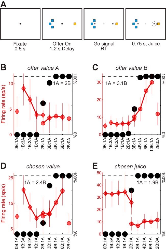
Behavioral task and cell groups. A: juice choice task. At the beginning of each trial, the animal fixated on the center of a screen. Two sets of colored squares, representing the two offers, appeared after 0.5 s. For each offer, the color indicated the juice identity, and the no. of squares indicated the juice quantity. The animal maintained center fixation for a randomly variable delay (1–2 s), after which the fixation point disappeared, and two saccade targets appeared by the offers (go cue). The animal indicated its choice with a saccade and maintained peripheral fixation for 0.75 s before juice delivery. B: neuron encoding the offer value A. The x-axis represents different offer types ranked by the ratio #B:#A. Black symbols represent the percent of “B” choices. Red symbols represent the neuronal firing rate (diamonds and circles indicate, respectively, choices of juice A and juice B). To highlight the variability in firing rates, thinner error bars here indicate the SD, and thicker error bars indicate the SE. C: neuron encoding the offer value B. D: neuron encoding the chosen value. E: neuron encoding the chosen juice. All conventions C–E are as in B.
We first examined the variability in the firing rate of individual neurons across trials. For each cell, we analyzed the relation between the mean spike count (μ) and its SD (σ). We began with the general assumption that σ and μ are related by a power law:
| (9) |
| (10) |
where α and β are constants. To estimate α and β, we took advantage of the fact that neuronal responses in OFC vary depending on the trial type. We computed μ and σ for each tuned cell, each time window, and each trial type. For each cell and each time window, we fit Eq. 10 using Deming's regression (see materials and methods) and we obtained αw and βw (Fig. 2A). We then averaged αw and βw across time windows to obtain an overall value of α and β for each cell. Across the population we found mean(α) = 0.679 ± 0.008 (Fig. 2B) and mean(β) = 1.12 ± 0.01. The measures of α and β were significantly correlated (Fig. 2C) and comparable to findings in visual cortex (Dean 1981; Vogels et al. 1989).
Fig. 2.

Neuronal variability in the orbitofrontal cortex (OFC). A: relation between mean firing rate (μ) and variance (σ) for one representative offer value cell (postoffer time window). Data are plotted in log scale, and each data point represents one trial type. The line is obtained from Deming's regression. For this response, αw = 1.0 and βw = −0.99. For each tuned cell (763 cells total), α and β were obtained averaging αw and βw across time windows. B: distribution of α. Across the population, mean(α) = 0.679 ± 0.008 (SE). C: relation between α and β. Each data point represents one neuron, and the two quantities are strongly anticorrelated. One outlier fell outside the range shown. D: relation between the Fano factor and the baseline activity. Baseline activity was defined as the firing rate in the preoffer time window. Each data point represents one neuron. Across the population, mean(Fano factor) = 1.8. E: relation between coefficient of variation (cv) and baseline activity. The two quantities are strongly anticorrelated. Across the population, mean(cv) = 1.0. F: time course of neuronal variability. Dark lines and shaded regions represent, respectively, the mean Fano factor and the corresponding SE (in sp/s). The Fano factor was calculated in 200-ms sliding windows. Neuronal variability dropped sharply shortly after the offer onset; it returned to the initial levels 500–700 ms after the offer; it decreased again and more mildly following the go signal and remained depressed until the trial end. The coefficient of variation presented a similar time course (data not shown).
One important metric for individual cells is provided by the relation between neuronal variability and firing rate. As apparent in Eq. 10, both α and β contribute to the variability, and both parameters are only defined for tuned cells. Therefore, to quantify this relation in all cells (including null cells), we analyzed the Fano factor and the coefficient of variation in relation to the baseline firing rate (preoffer time window). Population analyses revealed that the Fano factor varied only mildly with the baseline firing rate (Fig. 2D), whereas the coefficient of variation had a strong inverse relationship with the baseline firing rate (Fig. 2E).
Finally, we analyzed the time course of neuronal variability. We computed the Fano factor in 200-ms sliding time windows and averaged it across the entire population (Fig. 2F). The Fano factor dropped shortly after the offer and returned to baseline in the next 500–700 ms. It decreased again and more modestly after the go signal, remained depressed around juice delivery, and returned to baseline gradually in the 1 s following juice delivery. An analysis of the coefficient of variation provided a similar picture (data not shown). This result resonates with previous reports (Churchland et al. 2010), although neuronal variability in the OFC was previously found to drop only after juice delivery, whereas we observed the largest effect shortly after the offer. This discrepancy presumably reflects the fact that previous work focused on classical conditioning, whereas our monkeys were engaged in a choice task.
In summary, the firing rate of individual neurons in OFC was highly variable, and this variability was comparable to that typically measured in sensory areas.
Noise correlations in OFC are low.
Our dataset included 3,439 pairs of cells recorded simultaneously. Of these, 863 pairs were recorded from the same electrode, and 2,576 pairs were recorded from different electrodes placed at ≥1 mm distance. We computed the noise correlation (rnoise) for each cell pair. Across the population, rnoise ranged from −0.59 to 0.87, with mean(rnoise) = 0.019 ± 0.001 (average computed pooling time windows; Fig. 3A). Noise correlation strongly depended on interneuronal distance (P < 10−10, 1-way ANOVA). Pairs recorded from the same electrode had mean(rnoise) = 0.054 ± 0.004, while pairs at ≥1 mm distance had mean(rnoise) = 0.008 ± 0.001. To look at the effects of distance more closely, we binned pairs into four groups based on distance (Fig. 3B). Pairs recorded from the same electrode had significantly higher noise correlations than pairs at any of the greater distances (all P < 10−10, Tukey-Kramer test). Noise correlations did not decrease further at distances >1 mm (all P > 0.05, Tukey-Kramer test). Importantly, mean(rnoise) was significantly above zero in each time window, both at short distance (same electrode) and at long distance (different electrodes; all P < 10−3; t-test).
Fig. 3.

Noise correlation (rnoise) between pairs of neurons in OFC. A: overall distribution of rnoise. In this plot, we pooled all cell pairs and all time windows. Cell pairs with significant rnoise are indicated in dark. The rnoise differed significantly from zero for 1,592/3,439 (46%) cell pairs (P < 0.05; bootstrap analysis; see materials and methods). The black triangle below the x-axis marks the population average. For comparison, we indicate measures of noise correlation previously reported for middle temporal (MT) (Zohary et al. 1994), parietal areas 2/5 (Lee et al. 1998), M1 (Lee et al. 1998), V4 (Mitchell et al. 2009), and V1. For V1, the higher data point shown here is from Poort and Roelfsema (2009), and comparable measures were reported (Gutnisky and Dragoi 2008; Kohn and Smith 2005; Nienborg and Cumming 2006; Smith and Kohn 2008); the lower data point is from Ecker et al. (2010), and a comparable measure was reported (Ecker et al. 2014). B: values of rnoise grouped by interelectrode distance. The x-axis represents different time windows (see materials and methods). For all time windows, rnoise was significantly higher when the two cells were recorded from the same electrode. Notably, rnoise did not decrease beyond values measured at 1-mm distance. Error bars indicate SE. C: noise correlation as a function of the geometric mean of baseline firing rates. The geometric mean averaged across the population was 5.85 ± 0.09 sp/s (mean ± SE). Across the population, noise correlations were weakly but significantly correlated with the geometric mean of baseline firing rates (r = 0.05, P < 0.005; Spearman rank correlation). D: noise correlation as a function of the geometric mean of SDs. Population mean ± SE = 4.20 ± 0.04 sp/s. E: noise correlation as a function of the geometric mean of the coefficients of variation. Population mean ± SE = 1.048 ± 0.009. Data for C–E were taken from the preoffer time window. Note that values of rnoise for individual cell pairs fluctuate throughout the course of the trial and are negatively correlated with firing rate across time windows (see Fig. 4).
Notably, our measures of noise correlations were substantially smaller than those found in many previous studies of sensory and motor areas (Fig. 3A) (Gutnisky and Dragoi 2008; Kohn and Smith 2005; Lee et al. 1998; Liu et al. 2013; Nienborg and Cumming 2006; Poort and Roelfsema 2009; Smith and Kohn 2008; Smith and Sommer 2013; Zohary et al. 1994 but see Averbeck and Lee 2003; Ecker et al. 2014; Ecker et al. 2010; Mitchell et al. 2009; Miura et al. 2012). We thus examined several factors that might have artificially biased our estimates of noise correlation. First, because correlated activity may have variable timing, it is possible to underestimate noise correlations if the time windows for calculations are too small. However, the time windows used here (200–500 ms) were comparable to those used in many other studies and would capture the majority of correlated activity even if the timing of spikes varied stochastically over ∼100 ms (Cohen and Kohn 2011). For an additional control, we doubled the size of the time windows to 1 s and found that rnoise increased only by 15%. Second, imperfect spike sorting can bias measurements of rnoise. Specifically, when multiple cells are recorded on the same electrode, misassignment of spikes can create spurious correlations. However, this type of error would only apply to cells from the same electrode, and it would tend to inflate rather than reduce rnoise. Conversely, discarding meaningful spikes or mistakenly splitting spikes from one cell into several clusters could artificially lower rnoise. However, to decrease rnoise from 0.1 to the levels we observed in OFC, it would be necessary to discard >75% of spikes or to misidentify a single neuron as more than six separate cells (Cohen and Kohn 2011), which seems implausible. Third, firing rates in OFC are lower than in many other cortical areas (see below), and noise correlations tend to increase with firing rate (de la Rocha et al. 2007). Thus one possibility is that the discrepancy in rnoise reflected a genuine difference between areas, but was entirely due to the properties of individual cells as opposed to the network organization. However, additional analyses cast doubts on this view. Indeed, values of rnoise were comparable for pairs of tuned and null cells, despite the fact that null cells had lower firing rates throughout the trial. Furthermore, although the geometric mean of the firing rates was significantly related to rnoise in our dataset, this correlation was weak (Fig. 3C). Finally, our results can be compared with the predictions of a model relating noise correlation to firing rate (Cohen and Kohn 2011). The model predicts rnoise > 0.15 when both neurons have a firing rate of 1 sp/s. In our dataset, 90% of pairs had a baseline firing rate >1 sp/s for both neurons, while only 5% of pairs had rnoise > 0.15. In conclusion, differences in firing rates between OFC and sensory areas cannot fully explain the lower noise correlations found in OFC.
Time course of noise correlations.
We next examined how noise correlations varied over the course of a trial. A first analysis was based on seven large time windows. A repeated-measures ANOVA revealed that the strength of noise correlations varied systematically across time windows (P < 10−5; Fig. 3B). A post hoc analysis indicated that rnoise was significantly lower during the postoffer time window compared with the preoffer, delay, and pre-go time windows (P < 0.005; Tukey-Kramer test). Intermediate rnoise occurred during RT, prejuice, and postjuice time windows.
To analyze the time course of rnoise at higher resolution, we calculated rnoise in 200-ms sliding time windows. As illustrated in Fig. 4A, the mean(rnoise) dropped immediately after the offer presentation and returned to baseline levels ∼700 ms after the offer. It dropped again, but to a lesser extent, after the go signal, remained depressed until juice delivery, and returned to baseline gradually in the subsequent 1 s. Interestingly, the time profile measured for the correlated variability (Fig. 4A) closely resembled that measured for the variability of individual cells (Fig. 2E) and was inversely related to neuronal firing rate over the course of the trial (Fig. 4B). One concern might be whether transient decreases in noise correlation are caused by increases in firing rates. To address this issue, we restricted the analysis to cells whose firing rate decreased after the offer, and found that mean(rnoise) dropped after the offer even for these cells. Thus, the drop in rnoise observed in Fig. 4A was not simply a byproduct of higher firing rates.
Fig. 4.

Time course of noise correlation and firing rate. A: noise correlation. Values of rnoise were computed in 200-ms time windows slid by 25-ms intervals around offer presentation (left), go signal (middle), and juice delivery (right). Each data point is placed on the x-axis in the center of the corresponding time window. Dark lines and shaded regions indicate mean(rnoise) and SE, respectively. Noise correlations dropped sharply and transiently after the offer. This effect, most evident when neurons were recorded from the same electrode, was also observed when neurons were recorded from different electrodes. A second and more modest decrease in rnoise occurred after the go signal. This second drop was pronounced only in same-electrode pairs. Noise correlations gradually returned to baseline levels after juice delivery. All cell pairs in the dataset are included (863 same-electrode pairs, dark gray; 2,576 different-electrode pairs, light gray). B: firing rate. Shown is the firing rate averaged across all tuned cells (763 cells). All conventions as in A.
We next examined the time course of noise correlations as a function of the variables encoded by the two cells. Neurons in our dataset fell into four groups (offer value, chosen value, chosen juice, and null). These groups led to 10 pair types (Table 1). Figure 5A summarizes the values of rnoise observed for every pair type and time window. The time course of noise correlations was roughly consistent across pair types. In almost all cases, rnoise decreased in the postoffer time window compared with baseline, increased in the delay and pre-go time windows, decreased again after the go signal, and remained stable for the rest of the trial. Pairs of chosen juice neurons (pair type 3) presented an exception to this pattern. For these pairs, rnoise was lowest in the preoffer time window, with a nonsignificant increase after the offers were presented. This time course reflects a distinct feature of chosen juice neurons. Unlike other groups of neurons, chosen juice cells show in the preoffer time window a tail activity related to the outcome of the previous trial (Padoa-Schioppa 2013). Thus if two chosen juice cells have opposite juice preference, the tail activity introduces a negative correlation in the preoffer time window. This point can be observed in Fig. 5B, right, where pairs of chosen juice cells were divided based on whether they encoded the same juice (same polarity) or different juices (opposite polarity). Note that for pairs of chosen juice cells with the same polarity, the time course across time windows is similar to that observed for other pair types.
Fig. 5.

Noise correlations for different pair types. A: mean rnoise recorded for 10 pair types and 7 time windows. The no. of pairs for each pair type is indicated in Table 1, and colors indicate different time windows. Pooling time windows, rnoise varied significantly across pair type (P < 10−3, 1-way ANOVA). Post hoc tests found several significant differences in rnoise: type 1 > types 6–10, type 2 > types 7–9, type 3 > types 6–8, type 4 > types 7–9, and type 10 > types 7–8 (all P < 0.05, Tukey's least-significant difference). We also observed consistent trends across time windows. Starting from the preoffer time window (baseline), rnoise decreased in the postoffer time window. It then increased in the delay and pre-go time windows compared with the postoffer. It decreased again in the reaction time time window and remained roughly stable for the rest of the trial. These trends were observed for all pair types (with the exception of pair type 3 in the preoffer time window; see main text). B: mean rnoise for pair types 1-3, divided by juice polarity (see materials and methods). Pairs of neurons with the same polarity are on the left of each panel, while those with opposite polarities are on the right. For chosen juice pairs with opposite polarity, residual activity from the previous trial leads to negative noise correlations in the preoffer time window. C: mean rnoise by pair type. Data from different time windows are averaged separately for cell pairs recorded from the same electrode (top) and from different electrodes (bottom). All error bars indicate SE.
Noise correlations depend on the variables encoded by the two cells.
A primary goal of the study was to assess how noise correlations depend on the variables encoded by the two cells. To examine this issue, we first pooled data across time windows for each pair type (see Fig. 5A) and examined the entire population. A one-way ANOVA showed a significant effect of the pair type (P < 10−3). Mean(rnoise) was generally highest when two cells encoded the same variable (pair types 1–3) or were both null (pair type 10). However, rnoise was also relatively high for pairs of (offer value, chosen value) cells (pair type 4). We then broke down cell pairs depending on the distance between the two neurons (Fig. 5C). In these conditions, the pair type had a significant effect on rnoise when cells were from the same electrode (1-way ANOVA, P < 0.01). For cell pairs recorded on different electrodes, there was no significant effect of pair type (1-way ANOVA, P = 0.7). This finding suggests that the systematic pattern seen in Fig. 5A (the fact that noise correlations depended on the pair type) was influenced by the spatial distribution of cells. Indeed, the proportion of pairs found on the same electrode was about twice as high for pair types 1–4 and pair type 10 than it was for pair types 6–9 (see Table 1).
We further analyzed noise correlations between cells in the same group (offer value, chosen value, chosen juice). Specifically, we examined how rnoise depended on whether the two cells encoded the same juice or different juices, and how rnoise depended on the slope signs (positive or negative encoding). For offer value cells, the encoded juice and the slope sign were always unambiguous. For chosen juice cells, the design of experiment 1 made it impossible to distinguish between a cell encoding juice A with a positive slope and a cell encoding juice B with a negative slope (in both cases, the firing rate would be high/low for choices of juice A/B). We thus developed the concept of neuron polarity, which combined juice association and slope sign (see materials and methods). In essence, two cells had the same/opposite polarity if they “supported” the same/opposite decision. Our analyses showed that noise correlations were generally higher when two cells in the same group had the same polarity (Figs. 5B and 6, A and B). This pattern could be observed in both pairs from the same electrode and pairs from different electrodes [same electrode, P < 10−4; different electrode, P < 0.003; separate 2-way ANOVAs with factors (pair type × polarity)].
Fig. 6.

Noise correlations depend on the polarity of the two cells. A and C: cell pairs from the same electrode. B and D: cell pairs from different electrodes. A and B: noise correlations between cells in the same group (offer value, chosen value, and chosen juice). Black (white) bars refer to pairs of cells with the same (opposite) polarity. For each cell group, rnoise was higher when the two neurons had the same polarity. This observation was true both at short and long distance. C and D: noise correlations between pairs of offer value cells. Pairs were divided in 8 pools depending on whether the two cells were recorded from the same or different electrode (top, bottom), on whether the two neurons encoded the same juice or different juices (left, right), and on whether the sign of the encoding for the two cells was the same or different (dark gray, light gray). In general, rnoise was highest when two cells encoded the same juice with the same sign. Values of rnoise show the average across all time windows. Nos. in parentheses indicate the no. of neurons in each pool. All error bars indicate SE.
In the most granular analysis, we divided pairs of offer value cells in eight pools depending on whether the cells were recorded from the same or different electrodes, on whether the cells encoded the same juice or different juices, and on whether the sign of the encoding (positive or negative) was the same or different (Fig. 6, C and D). Although differences between groups were not statistically significant (t-test, all P > 0.05), it is interesting to note that noise correlations were highest when the two cells encoded the same juice with the same sign and progressively lower when the two cells encoded different juices with opposite signs, different juices with the same sign, and the same juice with opposite signs.
When two offer value cells encoded the same variable (same juice, same sign) and were recorded from the same electrode, mean(rnoise) was comparable to values seen in many sensory areas (Cohen and Kohn 2011). However, unlike neurons in sensory regions, offer value cells did not appear to cluster based on the encoded variable. Such a clustering would make it more likely to encounter pairs of offer value cells encoding the same variable (same juice, same sign) when two neurons are recorded from the same electrode compared with when two neurons are recorded ≥1 mm apart. In contrast, considering all pairs of offer value cells, 15/40 (38%) encoded the same variable when the two neurons were recorded from the same electrode, while 26/73 (34%) encoded the same variable when the two neurons were recorded from different electrodes (Fig. 6, C and D).
We do not know how sharply rnoise decays with distance, but it appears clear that the decay fully occurs within 1 mm (Fig. 3B). Because the area of OFC examined in our studies is relatively large (10–20 mm2 of cortex), most pairs of offer value cells are ≥1 mm apart. Hence, the results shown in Fig. 6D likely represent the typical rnoise for the majority of offer value cell pairs. Among these pairs, mean(rnoise) was highest when neurons encoded the same juice with the same sign. This gives rise to the difference in juice polarity seen in Fig. 6, A and B, and is particularly important for the remainder of the paper. If noise correlations within and between pools of offer value cells were balanced, stochastic fluctuations in different pools of neurons would be equal on average, and their effects on the decision would cancel. As a consequence, CPs would be at chance (Haefner et al. 2013; Nienborg et al. 2012). Thus the extent to which CPs of offer value cells differ from chance level is tightly related to the differences between the values shown in Fig. 6D.
Choice probabilities in OFC.
Current models posit that economic decisions are based on values computed in the OFC. In other words, offer value cells would provide the primary input to the decision. Consider a neuron that contributes to a decision process. In principle, stochastic fluctuations in the activity of the cell might be correlated with the decision made on any given trial. This correlation is quantified as a CP, which is essentially the probability with which an ideal observer would infer the decision outcome based only on the activity of the cell (Britten et al. 1996). At chance, CP = 0.5 and by convention CP > 0.5 (CP < 0.5) for neurons with positive (negative) encoding. We thus examined CP for offer value cells. To obtain an overall estimate for the population, we pooled neurons associated with the two juices (A and B), and we rectified the CP of offer value cells with negative encoding (see materials and methods). The distribution of CPs measured in the 500 ms after the offer was broad, with mean(CP) = 0.513 ± 0.007 (Fig. 7A). This value was higher than, but not statistically different from, 0.5 (P = 0.08; t-test). Importantly, CPs may be partly or fully explained by postdecision feedback. In principle, feedforward and feedback components of CPs can be disentangled based on a precise estimate of the decision time, which can be obtained in perceptual decisions using dynamic stimuli (Nienborg and Cumming 2009). However, economic decisions are not equally amenable to this approach because “stimuli” (i.e., offers) are entirely and unambiguously revealed as soon as they appear on the monitor. Importantly, when we quantified CPs focusing on an earlier and shorter time window [150–400 ms after the offer, as in a previous study (Padoa-Schioppa 2013)], we obtained a measure that was smaller but still >0.5 [mean(CP) = 0.507 ± 0.007].
All offer value cells associated to a given juice carry the same signal (they encode the same variable). However, from a decoding perspective, it would make sense if neurons with higher signal-to-noise ratio (higher neuronal sensitivity) had greater influence on the decision (higher CP). Indeed, a correlation between CP and neuronal sensitivity has been observed in sensory areas during perceptual decisions (Britten et al. 1996; Liu et al. 2013). We thus examined the relation between the CP and the neuronal sensitivity of individual cells across the population (Fig. 7B). For each offer value cell, the neuronal sensitivity was calculated dividing the tuning slope by the average SD. In this analysis, we pooled cells associated with the two juices (A and B), but we did not rectify cells with negative encoding (neuronal sensitivity < 0). CP and neuronal sensitivity were significantly correlated (r = 0.20, P < 0.003, Spearman rank correlation). We further quantified the relation between CP and sensitivity with a linear fit (y = a0 + a1x; Fig. 7B), which provided a linear term significantly greater than zero [a1 = 0.14; 95% confidence interval = (0.06, 0.21)]. To assess distortions from linearity, we also performed a fit using a third-order polynomial (y = a0 + a1x + a2x2 + a3x3; Fig. 7B). We found that terms a0 and a1 were significantly greater than zero (95% confidence interval) while terms a2 and a3 were statistically indistinguishable from zero (95% confidence interval). For a control, we repeated these analyses based on polarity (i.e., separating neurons associated with the two juices), and we obtained similar results. These analyses essentially fulfill the optimality test of Haefner et al. (2013). The results indicate that the readout of offer value cells does not differ significantly from an optimal scheme.
As previously noted (Padoa-Schioppa 2013), mean(CP) measured for offer value cells was substantially lower than the equivalent measure obtained for neurons in the middle temporal (MT) area during perceptual decisions (Britten et al. 1996; Cohen and Newsome 2009). At the same time, noise correlations between pairs of offer value cells were 5–10 times smaller than those measured in area MT under comparable conditions (Fig. 6, C and D). Importantly, a precise mathematical relation links noise correlations, CPs, and the readout weights of individual cells in a population. Within this computational framework, concurrent measures of noise correlations and CPs gave us the opportunity to investigate quantitatively the contribution of offer value cells to economic decisions.
Reconstructing choice probabilities from noise correlations.
Using Haefner's equation (Eq. 2), we conducted a series of simulations to assess whether noise correlations measured in the OFC, taken together with a plausible readout scheme of offer value cells, would induce a distribution of CPs close to that measured empirically. Specifically, we simulated CPs for a population of 10,000 offer value units. One-half of the units had positive polarity (representing positive encoding of juice A or negative encoding of juice B) and the other half had negative polarity (representing negative encoding of juice A or positive encoding of juice B). Noise correlations used in the simulations were computed from the empirical distributions measured for pairs of offer value cells during the postoffer time window (see materials and methods). We examined several readout schemes (see below). For each scheme, we considered two noise correlation matrices, referred to as long distance and “mixed-distance,” which effectively provided a lower bound and an upper bound for mean(CP) (see materials and methods).
Figure 7C summarizes the results of six simulations. First, we considered the simple case in which all units have equal magnitude weights (all ωi = ±1). CPs obtained from these simulations [long-distance mean(CP) = 0.528; mixed-distance mean(CP) = 0.542] were clearly above the empirical measure. Importantly, these simulations ignored a known source of choice variability, namely choice hysteresis (Padoa-Schioppa 2013). In essence, when two offers have similar values, monkeys were mildly biased toward the juice they chose in the previous trial. Choice hysteresis was quantified using a logistic analysis, and its effect was equivalent to multiplying the quantity of the previously chosen juice by 1.161. Most importantly, choice hysteresis was not reflected in the activity of offer value cells (Padoa-Schioppa 2013) and could thus be interpreted as an independent input to the decision. To account for choice hysteresis in the simulation, we incorporated two fictive units, one positive and one negative, corresponding to a previous choice of juice A or juice B, respectively. The relative weight of the two hysteresis units was derived mathematically starting from the estimate obtained from the logistic analysis, and was equal to ±0.161 times the cumulative weight of offer value units (see materials and methods). CPs obtained from these simulations [long-distance mean(CP) = 0.519; mixed-distance mean(CP) = 0.534; Fig. 7C] were closer to, but still above, the empirical measure.
Imposing uniform readout weights may be overly simplistic, since the brain could certainly take advantage of the heterogeneity in neuronal responses encoding a given offer value (Ecker et al. 2011). Indeed, the linear relation between CP and neuronal sensitivity across the population (Fig. 7B) suggests that the readout of offer value cells is close to optimal (Haefner et al. 2013). Thus, to complement our simulation analyses, we calculated the mean(CP) for a population of offer value units under the assumption of an optimal linear readout. Optimal readout weights were computed using Fisher's linear discriminant analysis, which finds the set of weights that best separates two conditions, in this case, choice A vs. choice B. These weights took into account the slope of the encoding measured for each neuron, as well as the response covariance measured across neurons. We thus computed the optimal readout weights for the population of offer value cells. CPs obtained from these simulations [long-distance mean(CP) = 0.502; mixed-distance mean(CP) = 0.502; Fig. 7C] were essentially at chance level and well below the empirical measure.
We repeated these analyses using a shorter time window (150–400 ms after offer onset) (Fig. 7D). Noise correlations, empirical CPs, and simulated CPs were all lower in this time window. Most importantly, the empirical measure of mean(CP) was very close to that obtained from the simulation using uniform weights and accounting for choice hysteresis (empirical = 0.507, simulated = 0.506).
To summarize, the CPs of offer value cells were lower than those typically measured in sensory areas during perceptual decisions. However, CPs were quantitatively as expected given the structure and the strength of noise correlations measured for pairs of offer value cells in OFC. The results obtained focusing on an earlier and shorter time window strengthen this conclusion.
DISCUSSION
Noise correlations in OFC are low.
Noise correlations in the OFC were on the order of 0.01. This measure is substantially lower than those reported for many cortical regions. Specifically, work in V1 (Gutnisky and Dragoi 2008; Kohn and Smith 2005; Nienborg and Cumming 2006; but see Ecker et al. 2010), V2 (Nienborg and Cumming 2006), MT (Cohen and Newsome 2009; Zohary et al. 1994), somatosensory area S2 (Romo et al. 2003), and primary motor cortex (Lee et al. 1998) has found noise correlations ranging 0.1–0.25. Studies in V4 (Cohen and Maunsell 2009; Mitchell et al. 2009) have reported intermediate levels of correlation (rnoise ≈ 0.03–0.07), which are closer to but still higher than those observed here for OFC. In lateral prefrontal cortex, noise correlations were smaller, but about twice the size of those found here (Constantinidis and Goldman-Rakic 2002). Importantly, many of these measures were obtained in awake behaving monkeys (Cohen and Newsome 2009; Gutnisky and Dragoi 2008; Nienborg and Cumming 2006, 2014; Poort and Roelfsema 2009; Zohary et al. 1994). Notable exceptions are the studies of Ecker and colleagues, who recently reported measures of rnoise in V1 comparable to those described here, and raised the hypothesis that high noise correlations measured in earlier studies may reflect factors such as spatial attention or task strategy (Ecker et al. 2014; Ecker et al. 2010 see also Gawne et al. 1996; Gawne and Richmond 1993). In this respect, it is worth emphasizing that our animals were actively engaged in a choice task. Moreover, since neurons in the OFC are not spatially tuned or associated with specific actions, factors such as spatial attention, action planning, or minor stimulus variability are unlikely to affect rnoise. Thus noise correlations in the OFC seem genuinely lower than those measured in sensory areas under comparable conditions. How can we explain this discrepancy?
Possibly important is the fact that our offers were always unequivocally defined. In contrast, studies of perceptual decisions often used stochastic stimuli (Liu et al. 2013; Nienborg and Cumming 2006; Poort and Roelfsema 2009; Zohary et al. 1994). In principle, specific realizations of a stochastic stimulus could elicit systematic neuronal responses (Bair and Koch 1996), which could result in overestimates of noise correlations (because noise correlations could partly reflect signal correlations). Independent of this consideration, at least two features distinguish OFC structurally and functionally from sensory areas. First, OFC lacks a clear position in a feedforward processing stream and, instead, integrates converging inputs from multiple sensory and limbic regions (Ongur and Price 2000). In contrast, sensory systems typically present hierarchical processing streams and are, by definition, predominantly unimodal. Theoretical analysis has suggested that correlations arise naturally across sequential stages of feedforward processing (Rosenbaum et al. 2010) and that hierarchical organization in itself may contribute to rnoise in many sensory areas. Consistent with this view, noise correlations in perirhinal cortex (Erickson et al. 2000) and in the supplemental motor area (SMA) (Averbeck and Lee 2003), both of which lack a clear hierarchical position, are low and comparable to those measured here. Second, aside from hierarchy, it remains unclear whether OFC has any topographic organization. As noted above, pairs of offer value cells encoding the same variable (same juice, same sign) were equally prevalent at short and long distances (Fig. 6, C and D), suggesting that any clustering is loose at best. At the same time, significant CPs are almost exclusively observed when the choice-relevant variable is topographically organized within a cortical area (Nienborg and Cumming 2014), suggesting that the circuit organization associated with a topographic map is a necessary condition to observe the patterns of noise correlation that induce high CPs. Interestingly, the rodent anterior piriform cortex (Miura et al. 2012), which also lacks any clear topography, is one of the few areas where rnoise is comparable to that measured here. However, noise correlations in SMA, an area with a clear topography, are also low (Averbeck and Lee 2003), indicating that topography is necessary but not sufficient to induce high noise correlations.
Despite differences in strength, noise correlations measured in the OFC presented several traits that clearly resembled those observed in other brain regions. First, rnoise was strongly affected by distance, falling off within 1 mm. A similar effect of distance was found in other cortical areas, although the decay was less sharp in V1 (Smith and Kohn 2008) and V4 (Smith and Sommer 2013). Second, as observed in sensory areas (Cohen and Newsome 2008; Liu et al. 2013; Smith and Kohn 2008), rnoise in OFC was highest when two neurons had similar tuning (i.e., when they encoded the same juice with the same sign). Notably, it is the “differential” component of noise correlations that ultimately limits the information encoded by a neuronal population (Abbott and Dayan 1999; Moreno-Bote et al. 2014; Shadlen et al. 1996). Third, the time course of noise correlations within a trial, specifically the fact that rnoise drops immediately after presentation of a relevant stimulus, is a common phenomenon (Carnevale et al. 2012; Churchland et al. 2010; Kohn and Smith 2005). In conclusion, it appears that noise correlations measured in OFC differ in strength, but not in structure, from those measured in other brain regions.
Noise correlations, choice probabilities, and the readout of offer value cells.
Current neuroeconomic models assume that decisions are based on subjective values computed in the OFC (Kable and Glimcher 2009; Padoa-Schioppa 2011; Rangel and Hare 2010; Rushworth et al. 2012). In the formalism of a linear decision model (Eq. 1), this means that the normalized readout weights of offer value cells should add to 1. Taking into account choice hysteresis, which provides a smaller but independent contribution to the decision, this proposition can be amended stating that normalized readout weights of each offer value pool should add to ∼0.839 in our task. To test this hypothesis, one would ideally measure readout weights directly, but this is not practically feasible. However, readout weights are quantitatively related to noise correlations and CPs, both of which can be measured. Based on this theoretical framework, we showed that the distribution of CPs measured for offer value cells can be reconstructed from concurrent measures of noise correlations assuming a plausible scheme of readout weights. More specifically, the empirical measure for mean(CP) fell between the values obtained with a uniform and with an optimal readout.
Our results provide a plausibility argument in favor of the hypothesis that offer value cells provide the primary input to economic decisions. Importantly, additional factors most likely affect the decision process. For example, previous results indicated that decisions are partly biased by the initial state of the neural assembly, reflected in the “predictive activity” of chosen juice cells (Padoa-Schioppa 2013). This predictive activity is largely a tail activity from the previous trial and is thus related to the behavioral phenomenon of choice hysteresis. Thus the fictive units in our simulations accounted for this source of choice variability. Conversely, our simulations did not include other possible sources of variability such as residual fluctuations in the initial state of the decision circuit, trial-by-trial fluctuations in the relative value of the goods (Padoa-Schioppa 2013), or downstream noise (Haefner et al. 2013). Most importantly, because any of those factors would reduce CPs, simulation analyses that accounted for any of them would effectively strengthen our current conclusions. The extent and implications of nonlinearities in the decoder remain to be examined. Exploring the fine structure and the mechanisms of the neural circuit that generates value-based decisions is a major goal for future research.
GRANTS
This work was supported by the National Institutes of Health (Grant nos. R01-DA-032758 and R01-MH-104494 to C. Padoa-Schioppa and T32-GM-008151 to K. E. Conen).
DISCLOSURES
No conflicts of interest, financial or otherwise, are declared by the authors.
AUTHOR CONTRIBUTIONS
Author contributions: K.E.C. and C.P.-S. conception and design of research; K.E.C. analyzed data; K.E.C. and C.P.-S. interpreted results of experiments; K.E.C. prepared figures; K.E.C. drafted manuscript; K.E.C. and C.P.-S. edited and revised manuscript; K.E.C. and C.P.-S. approved final version of manuscript; C.P.-S. performed experiments.
ACKNOWLEDGMENTS
We thank Ralf Haefner, Michael Shadlen, and John Assad for helpful discussions and comments on the manuscript.
REFERENCES
- Abbott LF, Dayan P. The effect of correlated variability on the accuracy of a population code. Neural Comput 11: 91–101, 1999. [DOI] [PubMed] [Google Scholar]
- Ahn S, Fessler JA. Globally convergent image reconstruction for emission tomography using relaxed ordered subsets algorithms. IEEE Trans Med Imaging 22: 613–626, 2003. [DOI] [PubMed] [Google Scholar]
- Averbeck BB, Lee D. Neural noise and movement-related codes in the macaque supplementary motor area. J Neurosci 23: 7630–7641, 2003. [DOI] [PMC free article] [PubMed] [Google Scholar]
- Bair W, Koch C. Temporal precision of spike trains in extrastriate cortex of the behaving macaque monkey. Neural Comput 8: 1185–1202, 1996. [DOI] [PubMed] [Google Scholar]
- Britten KH, Newsome WT, Saunders RC. Effects of inferotemporal cortex lesions on form-from-motion discrimination in monkeys. Exp Brain Res 88: 292–302, 1992. [DOI] [PubMed] [Google Scholar]
- Britten KH, Newsome WT, Shadlen MN, Celebrini S, Movshon JA. A relationship between behavioral choice and the visual responses of neurons in macaque MT. Vis Neurosci 13: 87–100, 1996. [DOI] [PubMed] [Google Scholar]
- Camille N, Griffiths CA, Vo K, Fellows LK, Kable JW. Ventromedial frontal lobe damage disrupts value maximization in humans. J Neurosci 31: 7527–7532, 2011. [DOI] [PMC free article] [PubMed] [Google Scholar]
- Carnevale F, de Lafuente V, Romo R, Parga N. Internal signal correlates neural populations and biases perceptual decision reports. Proc Natl Acad Sci USA 109: 18938–18943, 2012. [DOI] [PMC free article] [PubMed] [Google Scholar]
- Churchland MM, Yu BM, Cunningham JP, Sugrue LP, Cohen MR, Corrado GS, Newsome WT, Clark AM, Hosseini P, Scott BB, Bradley DC, Smith MA, Kohn A, Movshon JA, Armstrong KM, Moore T, Chang SW, Snyder LH, Lisberger SG, Priebe NJ, Finn IM, Ferster D, Ryu SI, Santhanam G, Sahani M, Shenoy KV. Stimulus onset quenches neural variability: a widespread cortical phenomenon. Nat Neurosci 13: 369–378, 2010. [DOI] [PMC free article] [PubMed] [Google Scholar]
- Cohen MR, Kohn A. Measuring and interpreting neuronal correlations. Nat Neurosci 14: 811–819, 2011. [DOI] [PMC free article] [PubMed] [Google Scholar]
- Cohen MR, Maunsell JH. Attention improves performance primarily by reducing interneuronal correlations. Nat Neurosci 12: 1594–1600, 2009. [DOI] [PMC free article] [PubMed] [Google Scholar]
- Cohen MR, Newsome WT. Context-dependent changes in functional circuitry in visual area MT. Neuron 60: 162–173, 2008. [DOI] [PMC free article] [PubMed] [Google Scholar]
- Cohen MR, Newsome WT. Estimates of the contribution of single neurons to perception depend on timescale and noise correlation. J Neurosci 29: 6635–6648, 2009. [DOI] [PMC free article] [PubMed] [Google Scholar]
- Constantinidis C, Goldman-Rakic PS. Correlated discharges among putative pyramidal neurons and interneurons in the primate prefrontal cortex. J Neurophysiol 88: 3487–3497, 2002. [DOI] [PubMed] [Google Scholar]
- de la Rocha J, Doiron B, Shea-Brown E, Josic′ K, Reyes A. Correlation between neural spike trains increases with firing rate. Nature 448: 802–806, 2007. [DOI] [PubMed] [Google Scholar]
- Dean AF. The variability of discharge of simple cells in the cat striate cortex. Exp Brain Res 44: 437–440, 1981. [DOI] [PubMed] [Google Scholar]
- Ecker AS, Berens P, Cotton RJ, Subramaniyan M, Denfield GH, Cadwell CR, Smirnakis SM, Bethge M, Tolias AS. State dependence of noise correlations in macaque primary visual cortex. Neuron 82: 235–248, 2014. [DOI] [PMC free article] [PubMed] [Google Scholar]
- Ecker AS, Berens P, Keliris GA, Bethge M, Logothetis NK, Tolias AS. Decorrelated neuronal firing in cortical microcircuits. Science 327: 584–587, 2010. [DOI] [PubMed] [Google Scholar]
- Ecker AS, Berens P, Tolias AS, Bethge M. The effect of noise correlations in populations of diversely tuned neurons. J Neurosci 31: 14272–14283, 2011. [DOI] [PMC free article] [PubMed] [Google Scholar]
- Erickson CA, Jagadeesh B, Desimone R. Clustering of perirhinal neurons with similar properties following visual experience in adult monkeys. Nat Neurosci 3: 1143–1148, 2000. [DOI] [PubMed] [Google Scholar]
- Gallagher M, McMahan RW, Schoenbaum G. Orbitofrontal cortex and representation of incentive value in associative learning. J Neurosci 19: 6610–6614, 1999. [DOI] [PMC free article] [PubMed] [Google Scholar]
- Gawne TJ, Kjaer TW, Hertz JA, Richmond BJ. Adjacent visual cortical complex cells share about 20% of their stimulus-related information. Cereb Cortex 6: 482–489, 1996. [DOI] [PubMed] [Google Scholar]
- Gawne TJ, Richmond BJ. How independent are the messages carried by adjacent inferior temporal cortical neurons? J Neurosci 13: 2758–2771, 1993. [DOI] [PMC free article] [PubMed] [Google Scholar]
- Glaister P. Least squares revisited. Math Gaz 85: 104–107, 2001. [Google Scholar]
- Gremel CM, Costa RM. Orbitofrontal and striatal circuits dynamically encode the shift between goal-directed and habitual actions. Nat Commun 4: 2264, 2013. [DOI] [PMC free article] [PubMed] [Google Scholar]
- Gutnisky DA, Dragoi V. Adaptive coding of visual information in neural populations. Nature 452: 220–224, 2008. [DOI] [PubMed] [Google Scholar]
- Haefner RM, Gerwinn S, Macke JH, Bethge M. Inferring decoding strategies from choice probabilities in the presence of correlated variability. Nat Neurosci 16: 235–242, 2013. [DOI] [PubMed] [Google Scholar]
- Hardin J, Garcia SR, Golan DA. Method for generating realistic correlation matrices. Ann Appl Stat 7: 1733–1762, 2013. [Google Scholar]
- Jeanne JM, Sharpee TO, Gentner TQ. Associative learning enhances population coding by inverting interneuronal correlation patterns. Neuron 78: 352–363, 2013. [DOI] [PMC free article] [PubMed] [Google Scholar]
- Kable JW, Glimcher PW. The neurobiology of decision: consensus and controversy. Neuron 63: 733–745, 2009. [DOI] [PMC free article] [PubMed] [Google Scholar]
- Kohn A, Smith MA. Stimulus dependence of neuronal correlation in primary visual cortex of the macaque. J Neurosci 25: 3661–3673, 2005. [DOI] [PMC free article] [PubMed] [Google Scholar]
- Lee D, Port NL, Kruse W, Georgopoulos AP. Variability and correlated noise in the discharge of neurons in motor and parietal areas of the primate cortex. J Neurosci 18: 1161–1170, 1998. [DOI] [PMC free article] [PubMed] [Google Scholar]
- Liu S, Gu Y, DeAngelis GC, Angelaki DE. Choice-related activity and correlated noise in subcortical vestibular neurons. Nat Neurosci 16: 89–97, 2013. [DOI] [PMC free article] [PubMed] [Google Scholar]
- Mitchell JF, Sundberg KA, Reynolds JH. Spatial attention decorrelates intrinsic activity fluctuations in macaque area V4. Neuron 63: 879–888, 2009. [DOI] [PMC free article] [PubMed] [Google Scholar]
- Miura K, Mainen ZF, Uchida N. Odor representations in olfactory cortex: distributed rate coding and decorrelated population activity. Neuron 74: 1087–1098, 2012. [DOI] [PMC free article] [PubMed] [Google Scholar]
- Moreno-Bote R, Beck J, Kanitscheider I, Pitkow X, Latham P, Pouget A. Information-limiting correlations. Nat Neurosci 17: 1410–1417, 2014. [DOI] [PMC free article] [PubMed] [Google Scholar]
- Nienborg H, Cohen MR, Cumming BG. Decision-related activity in sensory neurons: correlations among neurons and with behavior. Annu Rev Neurosci 35: 463–483, 2012. [DOI] [PubMed] [Google Scholar]
- Nienborg H, Cumming BG. Decision-related activity in sensory neurons may depend on the columnar architecture of cerebral cortex. J Neurosci 34: 3579–3585, 2014. [DOI] [PMC free article] [PubMed] [Google Scholar]
- Nienborg H, Cumming BG. Decision-related activity in sensory neurons reflects more than a neuron's causal effect. Nature 459: 89–92, 2009. [DOI] [PMC free article] [PubMed] [Google Scholar]
- Nienborg H, Cumming BG. Macaque V2 neurons, but not V1 neurons, show choice-related activity. J Neurosci 26: 9567–9578, 2006. [DOI] [PMC free article] [PubMed] [Google Scholar]
- Ongur D, Price JL. The organization of networks within the orbital and medial prefrontal cortex of rats, monkeys and humans. Cereb Cortex 10: 206–219, 2000. [DOI] [PubMed] [Google Scholar]
- Padoa-Schioppa C. Neurobiology of economic choice: a good-based model. Annu Rev Neurosci 34: 333–359, 2011. [DOI] [PMC free article] [PubMed] [Google Scholar]
- Padoa-Schioppa C. Neuronal origins of choice variability in economic decisions. Neuron 80: 1322–1336, 2013. [DOI] [PMC free article] [PubMed] [Google Scholar]
- Padoa-Schioppa C, Assad JA. Neurons in orbitofrontal cortex encode economic value. Nature 441: 223–226, 2006. [DOI] [PMC free article] [PubMed] [Google Scholar]
- Padoa-Schioppa C, Assad JA. The representation of economic value in the orbitofrontal cortex is invariant for changes of menu. Nat Neurosci 11: 95–102, 2008. [DOI] [PMC free article] [PubMed] [Google Scholar]
- Poort J, Roelfsema PR. Noise correlations have little influence on the coding of selective attention in area V1. Cereb Cortex 19: 543–553, 2009. [DOI] [PMC free article] [PubMed] [Google Scholar]
- Rangel A, Hare T. Neural computations associated with goal-directed choice. Curr Opin Neurobiol 20: 262–270, 2010. [DOI] [PubMed] [Google Scholar]
- Romo R, Hernandez A, Zainos A, Lemus L, Brody CD. Neuronal correlates of decision-making in secondary somatosensory cortex. Nat Neurosci 5: 1217–1225, 2002. [DOI] [PubMed] [Google Scholar]
- Romo R, Hernandez A, Zainos A, Salinas E. Correlated neuronal discharges that increase coding efficiency during perceptual discrimination. Neuron 38: 649–657, 2003. [DOI] [PubMed] [Google Scholar]
- Rosenbaum RJ, Trousdale J, Josic′ K. Pooling and correlated neural activity. Front Comput Neurosci 4: 9, 2010. [DOI] [PMC free article] [PubMed] [Google Scholar]
- Rudebeck PH, Saunders RC, Prescott AT, Chau LS, Murray EA. Prefrontal mechanisms of behavioral flexibility, emotion regulation and value updating. Nat Neurosci 16: 1140–1145, 2013. [DOI] [PMC free article] [PubMed] [Google Scholar]
- Rushworth MF, Kolling N, Sallet J, Mars RB. Valuation and decision-making in frontal cortex: one or many serial or parallel systems? Curr Opin Neurobiol 22: 946–955, 2012. [DOI] [PubMed] [Google Scholar]
- Shadlen MN, Britten KH, Newsome WT, Movshon JA. A computational analysis of the relationship between neuronal and behavioral responses to visual motion. J Neurosci 16: 1486–1510, 1996. [DOI] [PMC free article] [PubMed] [Google Scholar]
- Shadlen MN, Newsome WT. The variable discharge of cortical neurons: implications for connectivity, computation, and information coding. J Neurosci 18: 3870–3896, 1998. [DOI] [PMC free article] [PubMed] [Google Scholar]
- Smith MA, Kohn A. Spatial and temporal scales of neuronal correlation in primary visual cortex. J Neurosci 28: 12591–12603, 2008. [DOI] [PMC free article] [PubMed] [Google Scholar]
- Smith MA, Sommer MA. Spatial and temporal scales of neuronal correlation in visual area V4. J Neurosci 33: 5422–5432, 2013. [DOI] [PMC free article] [PubMed] [Google Scholar]
- Vogels R, Spileers W, Orban GA. The response variability of striate cortical neurons in the behaving monkey. Exp Brain Res 77: 432–436, 1989. [DOI] [PubMed] [Google Scholar]
- Wallis JD. Cross-species studies of orbitofrontal cortex and value-based decision-making. Nat Neurosci 15: 13–19, 2011. [DOI] [PMC free article] [PubMed] [Google Scholar]
- Xanthopoulos P, Pardalos P, Trafalis T. Linear discriminant analysis. In: Robust Data Mining. New York: Springer, 2013, p. 27–33. [Google Scholar]
- Zohary E, Shadlen MN, Newsome WT. Correlated neuronal discharge rate and its implications for psychophysical performance. Nature 370: 140–143, 1994. [DOI] [PubMed] [Google Scholar]