A SPECT imager with synthetic collimation

Abstract

This work outlines the development of a multi-pinhole SPECT system designed to produce a synthetic-collimator image of a small field of view. The focused multi-pinhole collimator was constructed using rapid-prototyping and casting techniques. The collimator projects the field of view through forty-six pinholes when the detector is adjacent to the collimator. The detector is then moved further from the collimator to increase the magnification of the system. The amount of pinhole-projection overlap increases with the system magnification. There is no rotation in the system; a single tomographic angle is used in each system configuration. The maximum-likelihood expectation-maximization (MLEM) algorithm is implemented on graphics processing units to reconstruct the object in the field of view. Iterative reconstruction algorithms, such as MLEM, require an accurate model of the system response. For each system magnification, a sparsely-sampled system response is measured by translating a point source through a grid encompassing the field of view. The pinhole projections are individually identified and associated with their respective apertures. A 2D elliptical Gaussian model is applied to the pinhole projections on the detector. These coefficients are associated with the object-space location of the point source, and a finely-sampled system matrix is interpolated. Simulations with a hot-rod phantom demonstrate the efficacy of combining low-resolution non-multiplexed data with high-resolution multiplexed data to produce high-resolution reconstructions.

1. INTRODUCTION

The most general mathematical description of a linear, digital imaging system is a continuous-to-discrete mapping^{1, 2}

$$g_m=\underset{S}{\int }f(r)h_m(r)d^{3}r+n_m,$$ (1)

where m = 1, …, M, and h_m(r) is the contribution to the m^th measurement from the object at point r, and n is the noise. The measurements g_m form the elements of a vector g in an M-dimensional space which we call the data space. The continuous distribution of radioactivity in object space is denoted by f. This continuous f is approximated with a discrete f by voxelizing the object. The imaging equation is then written as

$$\mathbf{g}=\mathbf{Hf}+\mathbf{n},$$ (2)

where H is the discrete system matrix that maps the object vector to an image, and the noise, n, is an M-dimensional vector in data space. Each element of H represents the probability that a photon emitted from a particular voxel is detected in a particular detector element.

Knowledge of the system matrix, H, of a single-photon emission computed tomography (SPECT) imaging system makes it possible to estimate the radiotracer distribution within an object from a set of detector measurements. There are many different reconstruction algorithms, but iterative algorithms that model the Poisson statistics of the data are becoming increasingly popular due to increased computational power, the development of accelerated methods, and the quality of the reconstructed images.^3–5 Iterative algorithms require an accurate forward model for object reconstruction. These methods work by making an initial estimate of the activity distribution and improving on this estimate with each iteration. The estimate is projected through the system and compared with the measured data. Correction terms are then calculated and are applied to update the current estimate. The estimate should become increasingly consistent with the measured data with each iteration.

Several methods have been proposed to experimentally measure the system matrix.^6–11 The most comprehensive method is to exhaustively measure the response of the system to a point source positioned at the center of each voxel. The detector response to a point source is known as the point spread function (PSF). The system matrix, H, is a concatenation of the PSFs for every voxel in the field of view (FOV). The resolution of the reconstructed image can be no finer than the sampling of the object space. It is very time consuming to experimentally measure a high-resolution system matrix. It may take several seconds to record a projection image and then translate the point source to the next voxel location. High-resolution small-animal SPECT systems typically require voxel sizes on the order of 0.5 mm or smaller. Experimentally measuring a system matrix with this resolution for any appreciable FOV could be prohibitively time consuming.

Typical multi-pinhole systems gather non-overlapping projection data from several pinholes onto one or more detectors.^{12, 13} Each pinhole images either the entire FOV or a small section of the FOV.¹⁴ Photons detected in detector elements with pinhole-projection overlap contain less information than counts in non-overlapping regions due to the ambiguity of their origin.^{15, 16} Multiplexing in the projection images can result in artifacts in the reconstruction.¹⁷ There is much interest in developing imaging systems that make use of overlapping multi-pinhole projections but do not suffer from artifacts.^{14, 18–20} The SPECT system discussed in this work, SyntheticSPECT, was developed to implement synthetic collimation for image formation and reconstruction.²¹ The synthetic-collimator method uses a multi-pinhole collimator because of its capability for high sensitivity and high resolution. The synthetic-collimator image is formed by estimating the activity distribution within the FOV and summing the activities in the voxels along the axis perpendicular to collimator face. This collimation method requires several projection images, each taken at a different system magnification, for the reconstruction. The high-magnification data are multiplexed, with several pinholes projecting the FOV onto the same detector element, while the low-magnification data are not multiplexed. Each system magnification is termed a “system configuration” in this paper because the magnification is controlled by adjusting the collimator-detector distance. There is no rotation in the system; a single tomographic angle is used in each system configuration. For SyntheticSPECT, the system matrix needs to be determined for every system configuration, and experimental measurement of multiple, finely-sampled system matrices is impractical.

The system matrix was measured by translating a point source through a sparsely-sampled grid in object space and the system response was recorded at each voxel for each system configuration. The pinhole projections were approximated with a Gaussian model. The multi-pinhole collimator used in this work projects the FOV onto the detector through forty-six pinhole apertures for the system configuration with lowest magnification. The pinhole projections were associated with their respective apertures in three-dimensional grids. Accurate aperture association was required to enable interpolation of the high-resolution data.²² The 3D grids were interpolated separately and later combined to form a finely-sampled system matrix.

The efficacy of combining multiplexed and non-multiplexed data was demonstrated with a hot-rod phantom imaging simulation. Projection data for six different magnifications were generated using an interpolated system matrix with cubic voxels of side-length 0.3125 mm. The hot-rod phantom was reconstructed using these projection data and an interpolated system matrix with cubic voxels of side-length 0.5 mm. Image reconstruction was performed using maximum-likelihood expectation-maximization (MLEM). The elements of the system matrix were generated on-the-fly, using a GPU, from the interpolated Gaussian coefficients of the pinhole projections.¹¹

2. METHODS

The SyntheticSPECT system (Fig. 1a) consists of a BazookaSPECT gamma-ray detector coupled to a fiber-optic taper.^{23, 24} The BazookaSPECT detector consists of a Lanex^® scintillator, image intensifier, optical lens, and a fast-frame-rate CCD camera. The sensor is operated at a high frame rate, or short exposure time, so that the optical photons associated with each gamma-ray interaction have a low probability of overlap. The CCD data are binned to a 320 × 240 array of 14.8 μm pixels. The effective optical pixel size is ~400 μm. Each photon interaction appears as a signal spread over a region of a few adjacent pixels, which is called a cluster. These pixel data are used to estimate the gamma-ray interaction location. A projection image may be formed by integrating these gamma-ray interaction positions.

Figure 1.

(a) An image of the SyntheticSPECT system. (b) A wireframe image of the multi-pinhole collimator. The 1 mm double-knife-edge pinholes are focused to a common field of view of ~25 mm. There are 110 pinhole apertures but only 46 apertures project the field of view onto the detector with the current 100 mm fiber-optic taper. (c) A typical integrated projection image for one voxel position. The voxel is in the corner of the FOV, and only the pinhole apertures that project this corner are imaged. There are 21 pinhole projections in this image. (d) The integrated projection image for all PSF voxel positions in the sparsely-sampled measurement grid. There is a sharp cutoff at the edge of the image due to the camera aperture. An insensitive area of the image intensifier is clearly seen in the center of one of the pinhole projections. (e) The integrated projection image for all PSF voxel positions in the interpolated grid. The edge of image has been masked due to errors in Gaussian fitting at the boundaries of (d). The insensitive part of the image intensifier at the center of one of the pinhole projections is masked due to inconsistencies in the fitting procedure.

The multi-pinhole collimator used in this work (Fig. 1b) has double-knife-edge (DKE) pinholes positioned in a pseudo-random pattern across the collimator, with a minimum inter-pinhole distance of 9 mm. Reconstruction artifacts may occur if multi-pinhole apertures are arranged in a symmetrical pattern.²⁵ The pinholes are 1.0 mm in diameter and are focused towards a 25 mm common FOV, but some pinholes also image areas outside of this space. For pinhole SPECT, H should contain information about the system geometry, attenuation and scattering of radiation in the object, radiometric factors, pinhole penetration, and detector blur. H can be obtained analytically, with Monte Carlo simulations, or with experimental measurements. In this work, the system matrix is experimentally measured by translating a point source (150 MBq ⁵⁷Co) through a cubic grid (30 × 30 × 30 mm³) encompassing the FOV and recording the system response at each voxel position. This system is designed to implement the synthetic collimator to produce a high-resolution reconstruction of an object using non-overlapping and overlapping projections.²¹ By combining projections of an object at different magnifications it has been shown experimentally that the effects of multiplexing may be mitigated.^{22, 26} Non-multiplexed data are acquired when the system magnification is low, and multiplexed data are acquired by increasing the magnification of the system. With a constant object-to-pinhole distance, the magnification of the system is controlled by adjusting the distance between the collimator and detector. Table 1 lists the approximate magnifications of the system for the six geometric configurations used in this work.

Table 1.

System configurations used in this work. The object-pinhole distance remained constant, and the magnification of the system was controlled by adjusting the pinhole-detector distance.

System Configuration	Object - Pinhole Distance, dOP (mm)	Pinhole - Detector Distance, dPD (mm)	Magnification
1	23	9	0.4
2	23	17	0.8
3	23	25	1.1
4	23	33	1.5
5	23	36	1.6
6	23	46	2.0

2.1 Gaussian Fitting

It is difficult to interpolate using the raw projection images. Instead, a 2D Gaussian distribution is fitted to the pinhole projections, and their coefficients are interpolated.^{2, 11} In SyntheticSPECT, each projection image has up to forty-six pinhole projections. Each of these pinhole projections must be identified and segmented.

The pinhole projections are first identified in each raw projection image using a thresholding algorithm. The resulting image is then filtered with a median filter to remove hot pixels. This processed image is used for finding the pinhole projections, but the raw image is used for fitting a distribution. The pinhole projections, and a small region of pixels surrounding them, are individually isolated in the raw projection image (Fig. 2a).

Figure 2.

(a) The pinhole projections in Fig. 1c are segmented. (b) A Gaussian distribution is fitted to each pinhole projection in (a), and each distribution is reprojected and centered.

The coefficients that characterize a 2D elliptical Gaussian distribution are the amplitude (A), the x coordinate (x̄), the y coordinate (ȳ), the x-width (σ_x), the y-width (σ_y), and the correlation coefficient (ρ). Estimates, and their upper and lower bounds, are made of these coefficients, and a 2D Gaussian fit is made to the cluster using a constrained non-linear optimization function in MATLAB^™ (“fmincon”). The number of counts in the distribution is preserved by applying a correction factor determined by the total signal in the raw and fitted clusters. The total signal in the fitted distribution can be found by reprojecting the distribution, or analytically using

$$\mathbf{Total}\mathbf{Counts}=A\times 2\pi \times {\sigma }_x\times {\sigma }_y\times \sqrt{(1-{\rho }^2)}.$$ (3)

The Gaussian distributions are reprojected in Fig. 2b. For this single voxel, storing the coefficients requires < 0.2% of the memory required to store the original projection image.

Each Gaussian distribution is then associated with its respective pinhole aperture. This association is done by identifying and tracking the pinhole projections as the point source is translated through the field of view.²² Each pinhole aperture is assigned a 3D grid (corresponding to the voxel grid) for each Gaussian coefficient (i.e., arrays of amplitudes (A), centroid positions (x̄,ȳ), x and y widths (σ_x, σ_y), and correlation coefficients (ρ)). Each of these 3D grids are interpolated to produce the full high-resolution system matrix.

2.2 Phantom Simulation

The effect of combining multiplexed and non-multiplexed data is demonstrated using simulated hot-rod phantom data. The diameter of the rods were 1.0, 1.2, 1.4, 1.6, 1.8 and 2.0 mm, and the distance between the centers of adjacent rods was equal to twice the diameter of the rods in that section (Fig. 3).

Figure 3.

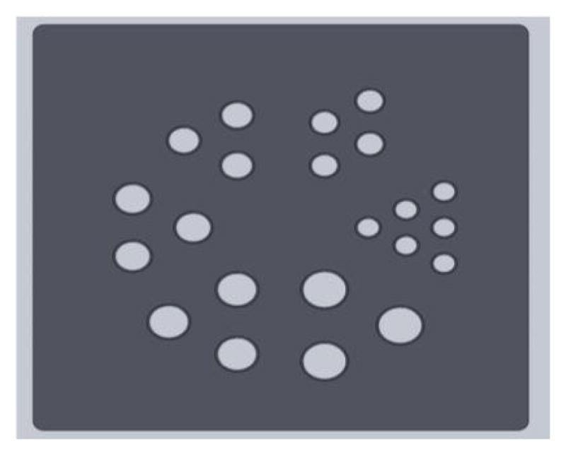
Image of the phantom used in this study. The diameters of the rods were 1.0, 1.2, 1.4, 1.6, 1.8, 2.0 mm, and the separation between the centres of the rods in each section was equal to twice the diameter of those rods. A background activity was also simulated.

The phantom was voxelized to a 3D grid with cubic voxels of side-length 0.3125 mm. An interpolated system matrix with this resolution was used to estimate the projection data for six system configurations. These projection data were then used to reconstruct the object on a 61 × 61 × 61 grid with cubic voxels of side-length 0.5 mm. The phantom had a uniform background, A_b, within the FOV. Each voxel within the rods had an activity, A_s, in addition to the background signal in the voxel. The signal contrast is defined as C = A_s / A_b. Fig. 4 shows the projection data for each system configuration when C = 0.15. Projection data were also generated for each system configuration when C = 0.50. The values of A_s and A_b in each test case were adjusted so that a total of 10⁷ counts were acquired.

Figure 4.

Projection data of the hot-rod phantom for system configurations: (a) 1, (b) 2,(c) 3,(d) 4,(e) 5 and (f) 6. The projection data were normalized to 10⁷ counts for each of the test cases. The level of overlap of the pinhole projections increases as the system magnification increases, but the number of projections subtended by the detector is reduced. A small circular insensitive area of the intensifier can clearly be seen in the same location in all images.

3. RESULTS

For each test case in Table 2.2, the hot-rod phantom was reconstructed using 400 iterations of the MLEM algorithm and post-smoothed with a Gaussian filter (Figs. 5 and 6). The edges of each of the reconstructions have been removed due to extreme values in the results of Test Case 2; the exteme values hid the central phantom area due to the image contrast. In each of the reconstructions there still appears to be some noise around edge of the images. The effects of noise are more apparent in Fig. 5 due to the lower signal contrast used in generating the projection data. Fig. 5a (Test Case 1) shows that the larger rods can be resolved using the non-multiplexed data. The smaller rods in the other sections of the phantom are not well resolved. Fig. 5b (Test Case 2) shows that multiplexed data cannot be used in isolation to reconstruct an object. Some rods may be visible in the reconstruction but there are also artifacts in the image. Fig. 5c (Test Case 3) shows that the deleterious effects of multiplexing may be negated and a high-resolution reconstruction acquired if highly multiplexed data are combined with non-multiplexed data. Fig. 5d (Test Case 4) shows that more rods are resolvable if more system configurations are used, even if those system configurations have magnifications that are within the range of those used in Test Case 3. The reconstructions of the hot-rod phantom using data with higher signal contrast (Fig. 6) are similar to those in Fig. 5.

Table 2.

Simulated test cases to demonstrate the effect of combining multiplexed and non-multiplexed data. The projection data from the different system configurations were used with an interpolated system matrix to reconstruct the hot-rod phantom.

Test Case	System Configurations
1	1
2	6
3	1 & 6
4	1, 2, 3, 4, 5 & 6

Figure 5.

The synthetic-collimator images for the four test cases: (a) Test Case 1, (b) Test Case 2, (c) Test Case 3 and (d) Test Case 4. The object (C = 0.15) was reconstructed using MLEM and the activities in the voxels were summed along the axis perpendicular to the collimator face. The edges of each of the images have been masked to highlight the contrast between the rods and the background. (b) suffers from extreme values near the edge of the FOV which would otherwise dominate the image.

Figure 6.

The synthetic-collimator images for the four test cases: (a) Test Case 1, (b) Test Case 2, (c) Test Case 3 and (d) Test Case 4. The object (C = 0.50) was reconstructed using MLEM and the activities in the voxels were summed along the axis perpendicular to the collimator face. The edges of each of the images have been masked to highlight the contrast between the rods and the background. (b) suffers from extreme values near the edge of the FOV which would otherwise dominate the image.

4. DISCUSSION AND CONCLUSION

This work presented the design and construction of a SPECT imaging system that uses synthetic collimation to estimate the activity distribution within the FOV. The system matrix was experimentally measured by translating a point source through a sparsely-sampled voxel grid encompassing the FOV. A 2D elliptical Gaussian distribution, characterized by six coefficients, was made to each pinhole projection for every voxel position. The coefficients were arranged in 3D grids corresponding to their respective pinhole apertures and the voxel position of the point source when the projection images were recorded. The system matrix was interpolated using the Gaussian coefficients. The interpolation has previously been validated through experimental work.²² The large number of pinhole projections, the irregular pinhole pattern, and the varying magnifications provide much information on an object distribution.

Fitting a Gaussian distribution to the pinhole projections was found to be suitable for each system magnification. The uncertainty in the 2D Gaussian fitting may be reduced by increasing the number of events detected for each voxel position. The number of events detected may be increased by improving detector efficiency with a thicker scintillator, by increasing the activity of the source, or by increasing the acquisition time. Increasing the frame rate of the CCD will reduce the probability of cluster overlap in each frame. Improved Gaussian fitting will result in a smoother, more accurate interpolation of the system matrix.

The accuracy of the system matrix is also reliant on the positioning of the X-Y-Z stage that translates the point source around the FOV. It is important that the positioning of these motors is reproducible to a subvoxel level. This accuracy must also be maintained for the imaging of extended objects. Synthetic collimation combines low-magnification and high-magnification data to estimate the activity distribution within the object. The X-Y positions of the motors must be the same for each system configuration, which is determined by the Z motor, to combine these data from different magnifications.

The non-multiplexed projection data produces low-resolution reconstructions, and highly-multiplexed data, when used on their own, do not allow for reconstruction of the object. The results of the hot-rod phantom simulation show that multiplexed data may be combined with non-multiplexed data to produce high-resolution reconstructions. According to the findings of Clarkson et al.,²⁷ the more data that is acquired from different system configurations, the better the estimates of the synthetic-collimator data. Further work is needed to determine the optimal number of system configurations for synthetic collimation.

References

- 1.Barrett HH, Myers KJ. Foundations of image science. John Wiley and Sons; 2004. [Google Scholar]
- 2.Chen YC, Furenlid LR, Wilson DW, Barrett HH. Small-Animal SPECT. Springer; 2005. pp. 195–201. Calibration of Scintillation Cameras and Pinhole SPECT Imaging Systems. [Google Scholar]
- 3.Shepp LA, Vardi Y. Maximum likelihood reconstruction for emission tomography. IEEE Trans Med Imaging. 1982;1(2):113–122. doi: 10.1109/TMI.1982.4307558. [DOI] [PubMed] [Google Scholar]
- 4.Hudson HM, Larkin RS. Accelerated image reconstruction using ordered subsets of projection data. IEEE Trans Med Imaging. 1994;13(4):601. doi: 10.1109/42.363108. [DOI] [PubMed] [Google Scholar]
- 5.Branderhorst W, Vastenhouw B, Beekman FJ. Pixel-based subsets for rapid multi-pinhole SPECT reconstruction. Phys Med Biol. 2010;55:2023–2034. doi: 10.1088/0031-9155/55/7/015. [DOI] [PubMed] [Google Scholar]
- 6.Rowe RK, Aarsvold JN, Barrett HH, Chen JC, Klein WP, Moore BA, Pang IW, Patton DD, White TA. A stationary hemi-spherical SPECT imager for three-dimensional brain imaging. Journal of Nuclear Medicine. 1993;34:474. [PubMed] [Google Scholar]
- 7.Beque D, Nuyts J, Bormans G, Suetens P, Dupont P. Characterization of acquisition geometry of pinhole spect. IEEE Trans Med Imaging. 2003;22:599–612. doi: 10.1109/TMI.2003.812258. [DOI] [PubMed] [Google Scholar]
- 8.Furenlid LR, Wilson DW, Chen Y, Kim H, Pietraski PJ, Crawford MJ, Barrett HH. Fast-SPECT II: a second-generation high-resolution dynamic SPECT imager. IEEE Trans Nucl Sci. 2004;51(3):631. doi: 10.1109/TNS.2004.830975. [DOI] [PMC free article] [PubMed] [Google Scholar]
- 9.van der Have F, Vastenhouw B, Rentmeester M, Beekman FJ. System calibration and statistical image reconstruction for ultra-high resolution stationary pinhole SPECT. IEEE Trans Med Imaging. 2008;27:960–971. doi: 10.1109/TMI.2008.924644. [DOI] [PubMed] [Google Scholar]
- 10.Defrise M, Vanhove C, Nuyts J. Perturbative refinement of the geometric calibration in pinhole SPECT. IEEE Trans Med Imaging. 2008;27:204–214. doi: 10.1109/TMI.2007.904687. [DOI] [PubMed] [Google Scholar]
- 11.Miller BW, Van Holen R, Barrett HH, Furenlid LR. A system calibration and fast iterative reconstruction method for next-generation SPECT imagers. IEEE Trans Nucl Sci. 2012b;59:1990–1996. doi: 10.1109/TNS.2012.2198243. [DOI] [PMC free article] [PubMed] [Google Scholar]
- 12.DiFilippo FP. Design and performance of a multi-pinhole collimation device for small animal imaging with clinical SPECT and SPECT-CT scanners. Phys Med Biol. 2008;53(15):4185–4201. doi: 10.1088/0031-9155/53/15/012. [DOI] [PMC free article] [PubMed] [Google Scholar]
- 13.Beekman FJ, van der Have F, Vastenhouw B, van der Linden AJA, van Rijk PP, Burbach JPH, Smidt MP. U-SPECT-I: a novel system for submillimeter-resolution tomography with radiolabeled molecules in mice. J Nucl Med. 2005;46(7):1194. [PubMed] [Google Scholar]
- 14.Schramm NU, Ebel G, Engeland U, Schurrat T, Behe M, Behr TM. High-resolution SPECT using multipinhole collimation. IEEE Trans Nucl Sci. 2003;50(3):315. [Google Scholar]
- 15.Defrise M, Gullberg GT. Review: Image reconstruction. Phys Med Biol. 2006;51(13):139–154. doi: 10.1088/0031-9155/51/13/R09. [DOI] [PubMed] [Google Scholar]
- 16.Barrett HH, Swindell W. Radiological Imaging: The theory of image formation, detection, and processing. Academic Press; 1981. [Google Scholar]
- 17.Nuyts J, Vunckx K, Defrise M, Vanhove C. Small animal imaging with multi-pinhole SPECT. Methods. 2009;48(2):83–91. doi: 10.1016/j.ymeth.2009.03.015. [DOI] [PubMed] [Google Scholar]
- 18.Vunckx K, Suetens P, Nuyts J. Effect of overlapping projections on reconstruction image quality in multipinhole SPECT. IEEE Trans Med Imaging. 2008;27(7):972. doi: 10.1109/TMI.2008.922700. [DOI] [PubMed] [Google Scholar]
- 19.Peterson TE, Furenlid LR. SPECT detectors: The anger camera and beyond. Phys Med Biol. 2011;56:R145–R182. doi: 10.1088/0031-9155/56/17/R01. [DOI] [PMC free article] [PubMed] [Google Scholar]
- 20.Mahmood ST, Erlandsson K, Cullum I, Hutton BF. The potential for mixed multiplexed and non-multiplexed data to improve the reconstruction quality of a multi-slit-slat collimator SPECT system. Phys Med Biol. 2010;55:2247–2268. doi: 10.1088/0031-9155/55/8/009. [DOI] [PubMed] [Google Scholar]
- 21.Wilson DW, Barrett HH, Clarkson EW. Reconstruction of two- and three-dimensional images from synthetic-collimator data. IEEE Trans Med Imaging. 2000;19:412–422. doi: 10.1109/42.870252. [DOI] [PubMed] [Google Scholar]
- 22.Havelin RJ, Miller BW, Barrett HH, Furenlid LR, Murphy JM, Dwyer RM, Foley MJ. Design and performance of a small-animal SPECT imaging system using synthetic collimation. Phys Med Biol. 2013;58:3397. doi: 10.1088/0031-9155/58/10/3397. [DOI] [PMC free article] [PubMed] [Google Scholar]
- 23.Miller BW, Barber HB, Barrett HH, Wilson DW, Chen L. A low-cost approach to high-resolution, single-photon imaging using columnar scintillators and image intensifiers. IEEE Nuclear Science Symposium Conference Record. 2006;6:3540–3545. [Google Scholar]
- 24.Miller, Barber HB, Barrett HH, Liu Z, Nagarkar VV, Furenlid LR. Progress in BazookaSPECT: high-resolution dynamic scintigraphy with large-area imagers. SPIE Optical Engineering + Applications. 2012a;8508:85080F. doi: 10.1117/12.966810. [DOI] [PMC free article] [PubMed] [Google Scholar]
- 25.Vunckx K, Beque D, Defrise M, Nuyts J. Single and multipinhole collimator design evaluation method for small animal SPECT. IEEE Trans Med Imaging. 2008;27:36–46. doi: 10.1109/TMI.2007.902802. [DOI] [PubMed] [Google Scholar]
- 26.Mahmood ST, Erlandsson K, Cullum I, Hutton BF. Experimental results from a prototype slit-slat collimator with mixed multiplexed and non-multiplexed data. Phys Med Biol. 2011;56:4311–4331. doi: 10.1088/0031-9155/56/14/007. [DOI] [PubMed] [Google Scholar]
- 27.Clarkson E, Barrett HH, Wilson DW. Synthesizing a parallel-projection image from pinhole data. SPIE. 1998;3336:251–259. [Google Scholar]