Genome-wide detection of intervals of genetic heterogeneity associated with complex traits

Abstract

Motivation: Genetic heterogeneity, the fact that several sequence variants give rise to the same phenotype, is a phenomenon that is of the utmost interest in the analysis of complex phenotypes. Current approaches for finding regions in the genome that exhibit genetic heterogeneity suffer from at least one of two shortcomings: (i) they require the definition of an exact interval in the genome that is to be tested for genetic heterogeneity, potentially missing intervals of high relevance, or (ii) they suffer from an enormous multiple hypothesis testing problem due to the large number of potential candidate intervals being tested, which results in either many false positives or a lack of power to detect true intervals.

Results: Here, we present an approach that overcomes both problems: it allows one to automatically find all contiguous sequences of single nucleotide polymorphisms in the genome that are jointly associated with the phenotype. It also solves both the inherent computational efficiency problem and the statistical problem of multiple hypothesis testing, which are both caused by the huge number of candidate intervals. We demonstrate on Arabidopsis thaliana genome-wide association study data that our approach can discover regions that exhibit genetic heterogeneity and would be missed by single-locus mapping.

Conclusions: Our novel approach can contribute to the genome-wide discovery of intervals that are involved in the genetic heterogeneity underlying complex phenotypes.

Availability and implementation: The code can be obtained at: http://www.bsse.ethz.ch/mlcb/research/bioinformatics-and-computational-biology/sis.html.

Contact: felipe.llinares@bsse.ethz.ch

Supplementary information: Supplementary data are available at Bioinformatics online.

1 Introduction

Genetic heterogeneity is the phenomenon that several distinct sequence variants may give rise to the same phenotype (Burrell et al., 2013); one refers to allelic heterogeneity if these variants are located in the same gene, and to locus heterogeneity if they occur in several distinct genes. This phenomenon is of the utmost importance to the exploration of the genetic basis of complex phenotypes, as most complex phenotypes have been found to be affected by numerous loci, rather than a single locus (McClellan and King, 2010).

The common ways of computing associations between genotype and phenotype are rather limited in their ability to detect genetic heterogeneity. Standard genome-wide association studies (GWAS) compute correlations between single genome positions, primarily single nucleotide polymorphisms (SNPs) and the phenotype of interest (Wellcome Trust Case Control Consortium, 2007). The smaller the sample size and the more SNPs that are involved in a phenotype, the less likely it is that genetic heterogeneity can be detected by this type of single-locus mapping. Gene-based tests quantify whether or not the number of sequence variants in one gene is enriched in cases versus controls (Neale and Sham, 2004). Although this approach does consider the combined effect of several SNPs, it is also restrictive in the sense that it only checks entire genes for association. It will miss any variants that lead to genetic heterogeneity, but are not located in or near the same gene.

Besides these two standard approaches to GWAS, many regression-based models for associating phenotype and genotype have been proposed, such as Lasso models (e.g. Kim et al., 2009). Although they are not limited to a single SNP or gene and thereby assess all possible loci at once, these models are limited in the sense that they cannot provide a measure of statistical significance for their findings on the level of sets of SNPs. At best, these models may provide a P-value that quantifies the probability that a certain SNP contributes to the phenotypic variance. But they cannot account for the inherent multiple hypothesis testing problem that is created by checking arbitrary contiguous intervals in the genome for genetic heterogeneity, let alone arbitrary sets of remote genetic loci.

The scale of this multiple testing problem in genetic heterogeneity search can be illustrated as follows: when considering all possible intervals in a genome in a dataset with 10⁶ SNPs, the number of tests one performs is quadratic in the number of SNPs in the genome, i.e. approximately $5\times {10}^{11}$ candidate intervals. When ignoring the multiple testing problem, one will obtain billions of false positives. If one performs the standard Bonferroni correction (Bonferroni, 1936), which divides the significance threshold α (typically 0.05 or 0.01) by the number of tests, then the corrected threshold will be so low that hardly any finding will be statistically significant.

We propose an algorithm for genome-wide detection of contiguous intervals that may exhibit genetic heterogeneity with respect to a given binary phenotype. More specifically, we search for genomic intervals in which the occurrence of at least one type of sequence variant (e.g. a point mutation or minority allele) is significantly more frequent in one of the two phenotypic classes. The fact that the sequence variant may occur at any SNP within the interval allows us to detect genetic heterogeneity in this manner. Our algorithm automatically finds the starting and end positions of these intervals, while properly correcting for multiple hypothesis testing and preserving statistical power. Central to this algorithm is an approach by Tarone (1990), which allows one to reduce the Bonferroni correction factor for multiple testing. We employ our novel algorithm on 21 binary phenotypes from Arabidopsis thaliana and discover intervals of SNPs in the Arabidopsis genome that are associated with 14 of these phenotypes, but could not be found with previous methods.

2 Approach

We will first state our problem formally, then provide the necessary background on statistical association testing and the multiple testing problem, before presenting our approach to genetic heterogeneity detection.

2.1 Problem statement: significant interval search

We are given a set of n individuals classified into two phenotypic groups, n₁ cases and n₂ controls (Fig. 1). Each individual is represented by an ordered sequence of L binary genotypes. The sequence of binary genotypes can represent binary SNPs in a homozygous setting or, more generally, a dominant/recessive encoding in a heterozygous setting.

Fig. 1.

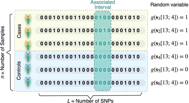
Schematic illustration of the problem of detecting genomic intervals that may exhibit genetic heterogeneity

Our goal is to find all genomic intervals, such that the occurrence of at least one genotype encoded as 1 (for instance, a minor allele or recessive genotype) within in each of these intervals is statistically significantly associated with the occurrence of a phenotype of interest.

The intervals found are promising candidates for regions of genetic heterogeneity underlying phenotypic variation and should be functionally investigated.

More formally, we are given a dataset ${\left\{(s_i,y_i)\right\}}_{i=1}^n$ where $s_i$ is the binary sequence of length L representing the i-th individual and $y_i\in \left\{\text{Cases},\text{Controls}\right\}$ is its corresponding binary phenotype. Each $s_i$ can itself be represented as an L-dimensional vector $s_i=(s_i[0],s_i[1],\dots ,s_i[L-1])$ with binary entries $s_i[j]\in \left\{0,1\right\}$. We denote the interval $(\tau ,l)$ of length l starting at index τ of a sequence $s_i$ as $s_i[\tau ;l]=(s_i[\tau ],s_i[\tau +1],\dots ,s_i[\tau +l-1])$. There are $\frac{L(L+1)}{2}$ possible intervals as we vary $l=1,\dots ,L$ and $\tau =0,\dots ,L-l$.

Finally, let $g(s_i[\tau ;l])$ be a binary random variable defined as $g(s_i[\tau ;l])=s_i[\tau ]\vee s_i[\tau +1]\vee \dots \vee s_i[\tau +l-1]$, where $\vee$ denotes the binary OR operator. Note that $g(s_i[\tau ;l])$ takes value 1 if the subsequence $s_i[\tau ;l]$ contains at least one non-zero entry and value 0 otherwise. Intuitively, $g(s_i[\tau ;l])$ indicates whether the i-th individual has one or more minor alleles in the genomic region determined by the interval $(\tau ,l)$ or not.

The problem we solve in this article is that of finding all intervals $(\tau ,l)$ with $l=1,\dots ,L$ and $\tau =0,\dots ,L-l$ such that the random variable $g(s[\tau ;l])$ is statistically associated with the phenotype y after correction for multiple hypothesis testing.

2.2 Statistical background

2.2.1 Statistical model

For each interval $(\tau ,l)$, the data ${\{g(s_i[\tau ;l]),y_i\}}_{i=1}^n$ can be arranged in the form of a 2 × 2 contingency table:

Variables	$g(s[\tau ;l])=1$	$g(s[\tau ;l])=0$	Row totals
$y=\text{Cases}$	$a_{\tau ,l}$	$n_1-a_{\tau ,l}$	n1
$y=\text{Controls}$	$x_{\tau ,l}-a_{\tau ,l}$	$n_2-(x_{\tau ,l}-a_{\tau ,l})$	n2
Col. totals	$x_{\tau ,l}$	$n-x_{\tau ,l}$	n

By the definition of $g(s[\tau ;l]),x_{\tau ,l}$ is the number of individuals in the dataset which have one or more minor alleles within the genomic interval $(\tau ,l)$. Similarly, $a_{\tau ,l}$ has the same interpretation but restricted only to cases.

In this article, the strength of the association between the phenotype y and the random variables $g(s[\tau ;l])$ will be evaluated using Fisher’s exact test (Fisher, 1922). We denote the P-value obtained by applying Fisher’s exact test to the 2 × 2 contingency table corresponding to the genomic interval $(\tau ,l)$ as $p_{\tau ,l}$. An interval $(\tau ,l)$ will be deemed to be significantly associated with the phenotype if $p_{\tau ,l}\le \delta$, with δ being the corrected significance threshold.

Our work can be readily extended to use other test statistics instead of Fisher’s exact test such as, for instance, the ${\text{χ}}^2$-test (Pearson, 1900).

2.2.2 Multiple hypothesis testing

To solve the significant interval search problem we must perform a statistical association test such as Fisher’s exact test for each of the $\frac{L(L+1)}{2}$ possible intervals $(\tau ,l)$. This means that for usual values of L in the order of 10⁵ or 10⁶, tens or hundreds of billions of hypotheses are being tested simultaneously.

This creates a challenging multiple hypothesis testing problem which would result in a crippling amount of false positives if multiple testing is not taken into account. Therefore, in this article, we chose to focus on approaches which strictly control the Family Wise Error Rate (FWER), defined as the probability of generating one or more false positives.

FWER control requires using testing procedures which guarantee that $\text{FWER}\le \text{α}$ with α being the desired significance level. To this end, one usually chooses the corrected significance threshold δ appropriately. Ideally, the optimal ${\delta }^{*}$ would be obtained by solving the following optimization problem

$${\delta }^{*}=\max \left\{\delta |\text{FWER}(\delta )\le \alpha \right\},$$

as it would yield the highest power, i.e. the probability of detecting true positives, while still strictly controlling the FWER.

However, since evaluating $\text{FWER}(\delta )$ in closed form is not possible in general, the most popular approaches resort to sub-optimal solutions. For instance, the well-known Bonferroni correction (Bonferroni, 1936) is equivalent to simplifying the original problem by using the bound $\text{FWER}(\delta )\le \delta D$, where D is the total number of statistical association tests being performed. When δD is used instead of $\text{FWER}(\delta )$ in the optimization problem above, it leads to the well-known correction ${\delta }_{\text{bon}}^{*}=\alpha /D$. Despite being popular due to its simplicity, the Bonferroni correction is often overly conservative, i.e. $\text{FWER}({\delta }_{\text{bon}}^{*})\ll {\delta }_{\text{bon}}^{*}D$ in practice. More importantly, in our setup where $D=\frac{L(L+1)}{2}$ is a huge number, the Bonferroni correction is too severely under-powered.

An alternative to the lack of power of the Bonferroni correction is to use permutation-testing methods, such as the Westfall–Young (WY) permutation testing procedure (Westfall and Young, 1993), to empirically estimate $\text{FWER}(\delta )$.

In WY permutation testing, we generate a resampled dataset by randomly permuting the class labels with respect to the individuals, obtaining a new dataset in which no interval is statistically associated with the (permuted) class labels. Then we compute the minimum P-value across all $\frac{L(L+1)}{2}$ intervals, $p_{\text{min}}={\min }_{(\tau ,l)}{p}_{\tau ,l}$, and compare it with δ. If $p_{\text{min}}>\delta$, then no interval is significant and there are no false positives in the resampled dataset; otherwise there are one or more false positives. If we repeat this a sufficiently large number of times J, obtaining J different minimum P-values ${\left\{p_{\text{min}}^{(j)}\right\}}_{j=1}^J$, one can compute an empirical estimate of the FWER as

$$\text{FWER}(\delta )=\frac{1}{J}{\displaystyle \sum _{j=1}^J\mathbb{1}\left[p_{\text{min}}^{(j)}\le \delta \right]},$$

where $\mathbb{1}$[•] takes value 1 if its argument is true and 0 otherwise. The optimal corrected significance threshold ${\delta }_{\text{wy}}^{*}$ which solves the original optimization problem can then be estimated as the α-quantile of the set ${\left\{p_{\text{min}}^{(j)}\right\}}_{j=1}^J$. Although the WY permutation testing procedure solves the power limitation of the Bonferroni correction by empirically estimating the high-dimensional dependence structure of the P-values for all $\frac{L(L+1)}{2}$ intervals, the computational effort required to compute ${\left\{p_{\text{min}}^{(j)}\right\}}_{j=1}^J$ is unfeasible for reasonable values of J, say 10³ or 10⁴. Although proving theoretically that the WY permutation-testing procedure achieves strong FWER control is challenging, often requiring the assumption of hard-to-verify technical conditions such as the subset pivotality condition, permutation-based testing is widely applied in computational biology as empirical evidence often suggests that strong FWER control is in fact achieved.

Next, we review the concept of the minimum attainable P-value for discrete test statistics, which we will extensively exploit in our contribution.

2.2.3 The concept of minimum attainable P-value

Tarone was the first to discuss in (Tarone, 1990) the existence of a minimum attainable P-value when discrete test statistics, such as Fisher’s exact test, are used. The idea is simple: since the test statistic is discrete, it can only take a finite set of values and there exists a minimum attainable P-value strictly greater than 0. As Tarone showed, one can exploit that to obtain an improved Bonferroni correction factor which exhibits a great increase in statistical power in many cases of interest.

In the context of 2 × 2 contingency tables, a large class of test statistics considers the table margins $x_{\tau ,l}$, n₁ and n₂ to be constant and, as a consequence, knowing the value of one of the four inner cell counts determines the value of the other three, i.e. the table has a single degree of freedom. Relevant examples are Fisher’s exact test, the ${\text{χ}}^2$-test and the Cochran–Mantel–Haenszel test (Mantel and Haenszel, 1959), among others. If we choose $a_{\tau ,l}$ as the cell count of reference (regardless of which of the four cell counts is chosen as the independent random variable one obtains exactly the same results, thus, we use $a_{\tau ,l}$ without loss of generality), then $a_{\tau ,l}\in \left\{a_{\text{min}},\dots ,a_{\text{max}}\right\}$ where $a_{\text{min}}=\max (0,x_{\tau ,l}-n_2)$ and $a_{\text{max}}=\min (x_{\tau ,l},n_1)$ are the minimum and maximum possible values of the cell count $a_{\tau ,l}$ consistent with the table margins. Thus, there are at most $a_{\text{max}}-a_{\text{min}}+1$ different attainable values for the test statistic and corresponding P-values. One can then compute the minimum attainable P-value as $\Psi (x_{\tau ,l},n_1,n_2)=\min \left\{p_{\tau ,l}(a_{\tau ,l},x_{\tau ,l},n_1,n_2)|a_{\tau ,l}\in [a_{\text{min}},a_{\text{max}}]\right\}$. (In our setup, the table marginals n₁ and n₂ are constant for all $\frac{L(L+1)}{2}$ intervals and only the margin $x_{\tau ,l}$ depends on the interval $(\tau ,l)$. Thus, we omit the dependence of $\Psi (x_{\tau ,l},n_1,n_2)$ on n₁ and n₂ from now on.)

The concept of the minimum attainable P-value $\Psi (x_{\tau ,l})$ has profound implications for multiple hypothesis testing problems involving discrete test statistics. Intuitively, it quantifies the strongest association that we could ever observe just based on the table margins. When applied to the significant interval search problem, if $\Psi (x_{\tau ,l})>\delta$ then we know that the interval $(\tau ,l)$ can never be significant regardless of the actual value of $a_{\tau ,l}$. More importantly, when test statistics are used which consider the table margins fixed, one can prune those intervals from the search space without affecting the FWER.

More formally, we define ${\mathcal{I}}_T(\delta )=\{(\tau ,l)|\Psi (x(\tau ,l))\le \delta \}$ as the set of testable intervals at corrected significance level δ. All intervals which are not in ${\mathcal{I}}_T(\delta )$ can never achieve significance at level δ and are thus called non-testable at that level. The FWER at significance level δ can then be upper bounded by $\delta \left|{\mathcal{I}}_T(\delta )\right|$, motivating the following procedure to find the corrected significance threshold ${\delta }^{*}$:

$${\delta }_{\text{tar}}^{*}=\max \left\{\delta |\delta \left|{\mathcal{I}}_T(\delta )\right|\le \alpha \right\}$$

Like the Bonferroni correction, Tarone’s method also ignores the dependence structure between test statistics, thus being less powerful than permutation-based testing approaches. On the other hand, by exploiting the discreteness of the test statistic, it has greatly increased statistical power when compared with a standard Bonferroni correction. The method as proposed by Tarone had to be solved by a brute-force approach requiring computation of the minimum attainable P-values for every single test. When a very large number of tests have to be performed, that is unfeasible due to the daunting computational complexity involved. Nonetheless, by carefully designing context-dependent pruning techniques, Tarone’s method was successfully applied recently to association rule mining (Minato et al., 2014; Terada et al., 2013) and graph mining (Sugiyama et al., 2015).

However, all of those approaches cannot work directly with the exact minimum attainable P-value function $\Psi (x)$. Instead, they used a surrogate function $\widehat{\Psi }(x)$ which greatly overestimates the potential for significance when the margin x is close to n. Since that situation is commonly encountered in the significant interval search problem, especially for sufficiently large intervals, the existing methods cannot be readily extended to our task.

Next, we present our contribution: two alternative algorithms to solve the significant interval search problem by making use of the exact minimum attainable P-value; one based on Tarone’s method and another on WY permutation testing.

2.3 Our approach: significant interval search with fast automatic interval search and FAIS-WY

Here, we describe the Fast Automatic Interval Search (FAIS) algorithm and its Westfall–Young-based counterpart, FAIS-WY. Both methods exploit the concept of minimum attainable P-value reviewed in Section 2.2.3 along with a novel pruning technique to obtain a corrected significance threshold ${\delta }^{*}$ for the significant interval search problem. However, their exact goal differs: FAIS provides a computationally efficient way to apply Tarone’s method to the significant interval search problem whereas FAIS-WY makes applying the WY permutation testing procedure to the significant interval search problem feasible. That is, FAIS computes ${\delta }_{\text{tar}}^{*}$ whereas FAIS-WY computes ${\delta }_{\text{wy}}^{*}$. In practice, FAIS-WY is more computationally demanding than FAIS but has increased statistical power.

Algorithm 1. FAIS and FAIS-WY main body.

1: function Main

2:   init_specific()

3:   $\mathrm{interval\_queue}\leftarrow \left\{(0,1),(1,1),\dots ,(L-1,1)\right\}$

4:   Set $k\leftarrow 1$ and compute δ_k, Σ_k and ${\sigma }_l^k$

5:   while $\mathrm{interval\_queue}$ is not empty do

6:    $(\tau ,l)\leftarrow \mathrm{intervalqueue}\mathrm{.pop()}$

7:    Compute $g(s_i[\tau ;l])\forall i=1,\dots ,n$

8:    $x_{\tau ,l}={\sum }_{i=1}^{n}g(s_i[\tau ;l])$

9:    if $x_{\tau ,l}\in {\Sigma }_k$ then

10:     process_interval_specific()

11:    end if

12:    if $x_{\tau ,l}\le n-{\sigma }_l^k$ and $x_{\tau -1,l}\le n-{\sigma }_l^k$ then

13:     $\mathrm{intervalqueue}\mathit{.append}((\tau -1,l+1))$

14:    end if

15:  end while

16: end function

The main body of FAIS and FAIS-WY is presented as Algorithm 1, which emphasizes the common structure between both methods. The general idea is to initialize the tentative corrected significance threshold δ to the largest possible value such that all intervals are initially testable. Intervals $(\tau ,l)$ are then sequentially enumerated in increasing order of length and, if they are testable at the current level δ, they are processed leading to an adjustment of δ to ensure that the respective FWER-related target is satisfied: $\delta \left|{\mathcal{I}}_T(\delta )\right|\le \alpha$ for FAIS and $\text{FWER}(\delta )\le \alpha$, with $\text{FWER}(\delta )$ estimated via WY-permutations for FAIS-WY. Finally, intervals are pruned from the search space, if possible.

Therefore, we need to have an efficient way to check whether an interval $(\tau ,l)$ is testable and a way to determine when all intervals containing the current interval $(\tau ,l)$ can be pruned from the search space. We address each of those points next.

2.3.1 Testability

Let $\{{\delta }_0,{\delta }_1,\mathrm{...},{\delta }_{\lfloor \frac{n}{2}\rfloor }\}$ be the image of $\Psi (x)$ sorted in a monotonically decreasing sequence. Notice that there are only $\lfloor \frac{n}{2}\rfloor +1$ different values because $\Psi (x)$ is symmetric around $n/2$ (Fig. 2). Now, we define the testable region $\Sigma (\delta )$ as the set $\Sigma \left(\delta \right)\subset \left[0,n\right]$ such that $x_{\tau ,l}\in \Sigma (\delta )\iff (\tau ,l)\in {\mathcal{I}}_T(\delta )$. In other words, the interval $(\tau ,l)$ is testable at level δ if and only if the margin $x_{\tau ,l}$ of interval $(\tau ,l)$ belongs to $\Sigma (\delta )$. Two important properties of the testable regions $\Sigma (\delta )$ are:

Property 1 —

$\forall \delta \in [{\delta }_k,{\delta }_{k-1}),{\mathcal{I}}_T(\delta )={\mathcal{I}}_T({\delta }_k)\Rightarrow \Sigma (\delta )=\Sigma ({\delta }_k)\equiv {\Sigma }_k$

Property 2 —

(i) if ${\delta }_k<\Psi (\lfloor \frac{n}{2}\rfloor )$, the region Σ_k is the union of two symmetric intervals, i.e. ${\Sigma }_k=[{\sigma }_l^k,{\sigma }_u^k]\cup [n-{\sigma }_u^k,n-{\sigma }_l^k]$; (ii) if ${\delta }_k\ge \Psi (\lfloor \frac{n}{2}\rfloor )$ the region is composed of a single interval, ${\Sigma }_k=[{\sigma }_l^k,n-{\sigma }_l^k]$.

Fig. 2.

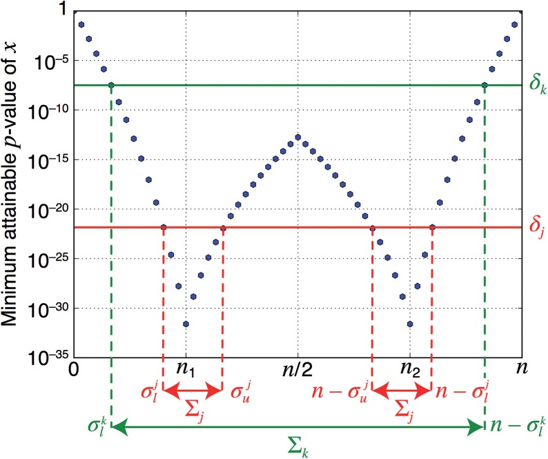
Minimum attainable p-value Ψ(x) for n = 60, n₁ = 15 (blue dots)

Property 1 states that, since $\Psi (x)$ attains only $\lfloor \frac{n}{2}\rfloor +1$ different values, there are only $\lfloor \frac{n}{2}\rfloor +1$ different sets of testable intervals ${\mathcal{I}}_T(\delta )$ and corresponding testable regions $\Sigma (\delta )$. Thus, it suffices to consider only the $\lfloor \frac{n}{2}\rfloor +1$ cases corresponding to $\{{\delta }_0,{\delta }_1,\mathrm{...},{\delta }_{\lfloor \frac{n}{2}\rfloor }\}$ defined above, with testable regions $\Sigma ({\delta }_k)\equiv {\Sigma }_k$.

Property 2, along with the symmetry of $\Psi (x)$, implies that the regions $\Sigma ({\delta }_k)$ are easy to describe and can in fact be computed by starting from $\Sigma ({\delta }_0)=[0,n]$ and iteratively ‘shrinking’ them to obtain $\Sigma ({\delta }_k)$ from $\Sigma ({\delta }_{k-1})$. The computational complexity of each such step is negligible (O(1)). The two different shapes that testable regions Σ_k can take are described in Figure 2.

In summary, to check if an interval $(\tau ,l)$ is testable at level $\delta \in [{\delta }_k,{\delta }_{k-1})$ one just needs to check if $x_{\tau ,l}\in {\Sigma }_k$ or not.

2.3.2 Pruning

We exploit the following fact: intervals $({\tau }^{\prime },l^{\prime })$ containing the interval $(\tau ,l)$ have margins $x_{{\tau }^{\prime },l^{\prime }}\ge x_{\tau ,l}$. Thus, if the interval $(\tau ,l)$ is non-testable and $x_{\tau ,l}>n-{\sigma }_l^k$, no interval containing it can be testable and we can prune the search space. Notice that an interval $(\tau ,l)$ can be non-testable, i.e. $x_{\tau ,l}\cancel{\in }{\Sigma }_k$, and yet the search space will not be pruned if $x_{\tau ,l}<n-{\sigma }_l^k$.

Thus, if we enumerate intervals in increasing order of length, every time an interval with $x_{\tau ,l}>n-{\sigma }_l^k$ is found to be non-testable, any other interval which contains it can be deemed to be non-testable too without needing to inspect it.

2.3.3 Detailed description of the pseudocode

Next, we describe in greater detail the pseudocode common to FAIS and FAIS-WY in Algorithm 1 in order to discuss the specific aspects of each of the two algorithms.

Initialization: In Line 2 the variables specific to FAIS or FAIS-WY are initialized. Key to the enumeration procedure is the variable interval_queue, which is initialized in Line 3 by pushing all length 1 intervals. Finally, the tentative corrected significance threshold is initialized to $\delta ={\delta }_1$, which is the largest value that $\Psi (x)$ can take other than the trivial value ${\delta }_0=1$, and the corresponding testability region Σ_k and its left-most point ${\sigma }_l^k$ is obtained.

Enumeration process: Between lines 5 and 15 one finds the core of the algorithm; a while loop which analyzes the intervals contained in the queue one by one, iteratively adding new intervals which cannot be pruned to the queue during the process. The loop naturally stops once the queue becomes empty.

Within the loop, first of all, the interval $(\tau ,l)$ located at the head of the queue is popped (Line 6). The values of the random variable $g(s_i[\tau ;l])$ are then evaluated for all n individuals, and the corresponding margin $x_{\tau ,l}$ is computed (Lines 7 and 8). Next, in Line 9, one checks if the interval $(\tau ,l)$ is testable at the current corrected significance level δ_k. If $x_{\tau ,l}\cancel{\in }{\Sigma }_k$, then the interval is not testable and does not need to be processed. In contrast, if $x_{\tau ,l}\in {\Sigma }_k$, the interval is testable at the current significance threshold δ_k and we must process it, appropriately decreasing δ_k and shrinking Σ_k, thus also decreasing $n-{\sigma }_l^k$. How that processing step is made is what sets FAIS and FAIS-WY apart algorithmically and statistically and will be discussed later.

Finally, pruning occurs in Line 12. We know that if either the current interval being processed $(\tau ,l)$ or the preceding interval $(\tau -1,l)$ are non-testable with margin $x>n-{\sigma }_l^k$, then the interval $(\tau -1,l+1)$ cannot possibly be testable and does not need to be appended to the queue of intervals to be processed. Note also that if either interval $(\tau ,l)$ or interval $(\tau -1,l)$ had been previously pruned due to this criteria, interval $(\tau -1,l+1)$ will be pruned too. In other words, pruning propagates from shorter intervals to longer length intervals containing them. As $n-{\sigma }_l^k$ decreases as intervals are processed, the algorithm naturally ends after all testable intervals at the final ${\delta }^{*}$ have been enumerated.

FAIS specific functions: In Algorithm 2, we describe how FAIS processes the testable intervals. The key idea is to keep an n + 1-dimensional vector of counters c, originally initialized with all zero entries, such that $c[k]$ is the number of intervals processed so far which had $x_{\tau ,l}=k$. Thus, ${\sum }_{x\in {\Sigma }_k}c[x]$ equals the number of testable intervals at the corrected significance threshold δ_k found so far.

Every time a new testable interval $(\tau ,l)$ is found, the corresponding counter $c[x_{\tau ,l}]$ is increased by one making the improved Bonferroni bound $({\sum }_{x\in {\Sigma }_k}c[x]){\delta }_k$ increase too. If the bound is still lower than α, nothing needs to be done. However, when it becomes larger, we know that the current testability threshold δ_k is too large. Thus, in line 7, we increase k, reducing δ_k and effectively shrinking the testability region Σ_k until the condition $({\sum }_{x\in {\Sigma }_k}c[x]){\delta }_k\le \alpha$ is satisfied again.

Algorithm 2. FAIS specific functions.

1: function init_FAIS

2:   $c\leftarrow 0_{n+1}$

3: end function

4: function process_interval_FAIS

5:   $c[x(\tau ,l)]\leftarrow c[x(\tau ,l)]+1$

6:   while $({\sum }_{x\in {\Sigma }_k}c[x]){\delta }_k>\alpha$ do

7:    Set $k\leftarrow k+1$ and recompute δ_k, Σ_k and ${\sigma }_l^k$

8:   end while

9: end function

FAIS-WY specific functions: At initialization, we generate all J shuffled phenotypes ${\left\{y^{(j)}\right\}}_{j=1}^J$ at once and initialize ${\left\{p_{\text{min}}^{(j)}\right\}}_{j=1}^J$. Upon finding a testable interval, one must compute the corresponding Fisher’s exact test P-values for all J randomly shuffled phenotype vectors ${\left\{y^{(j)}\right\}}_{j=1}^J$, updating the minimum P-values across all intervals processed so far, ${\left\{p_{\text{min}}^{(j)}\right\}}_{j=1}^J$ if needed. Then, the condition for decreasing the threshold simply becomes $\text{FWER}(\delta )>\alpha$, where $\text{FWER}(\delta )$ is the empirical FWER estimation obtained using the J minimum P-values obtained so far.

Algorithm 3. FAIS-WY specific functions.

1: function init_FAIS-WY

2:   for $j=1,\dots ,J$ do

3:    $y^{(j)}\leftarrow \text{rand}\_\text{permute}(y)$

4:    $p_{\text{min}}^{(j)}\leftarrow 1$

5:   end for

6: end function

7: function process_interval_FAIS-WY

8:   for $j=1,\dots ,J$ do

9:    Compute $p_{\tau ,l}^{(j)}$

10:    $p_{\text{min}}^{(j)}\leftarrow \min (p_{\text{min}}^{(j)},p_{\tau ,l}^{(j)})$

11:  end for

12:  while $\text{FWER}(\delta )>\alpha$ do

13:    Set $k\leftarrow k+1$ and recompute δ_k, Σ_k and ${\sigma }_l^k$

14:  end while

15: end function

This approach is well-defined mainly due to two properties of the FWER estimator: (i) if the significance threshold δ_k remains fixed, inspecting a new interval can never make $\text{FWER}({\delta }_k)$ decrease; and (ii) $\text{FWER}(\delta )$ can be evaluated exactly for all $\delta \le {\delta }_k$ using only the set of intervals satisfying $x_{\tau ,l}\in {\Sigma }_k$. Thanks to those two properties, the algorithm follows an iterative cycle of interval enumeration, FWER estimation and significance threshold adjustment which continues until all intervals belonging to a certain ${\Sigma }_{k^{*}}$ have been enumerated. Finally, ${\delta }^{*}$ can be obtained as the α-quantile of ${\left\{p_{\text{min}}^{(j)}\right\}}_{j=1}^J$.

2.3.4 Enumeration of significant intervals

Once the corrected significance threshold ${\delta }^{*}$ has been obtained, either with FAIS or FAIS-WY, we execute a slightly modified version of Algorithm 1 so that δ_k in Line 4 is directly initialized to ${\delta }^{*}$. Then the process_interval() function evaluates $a_{\tau ,l}={\sum }_{i|y_i=1}g(s_i[\tau ;l])$, computes the corresponding P-value according to Fisher’s exact test and outputs those intervals such that $p_{\tau ,l}\le {\delta }^{*}$. Note that in this case, the significance threshold δ_k does not change along the execution of the algorithm.

2.3.5 Filtering of overlapping significant intervals

Due to the way the problem is formulated, it is common to have clusters of overlapping significant intervals which introduce redundancy in the findings. As a post-processing step, only the most significant interval in the cluster, i.e. the one with the smallest P-value, is kept. As the most significant interval is guaranteed to be kept by this post-processing scheme, the FWER is unchanged and thus the computation of the significance threshold ${\delta }^{*}$ is unaffected. We illustrated this filtering process in Figure (Supplementary Fig. S1).

3 Experiments

We evaluate the ability of FAIS and FAIS-WY to detect genome-wide contiguous intervals that may exhibit genetic heterogeneity on simulated data as well as on data from an association mapping study in Arabidopsis thaliana. As benchmarks, we use BRUTE, the ‘brute force’ method using the Bonferroni correction, BRUTE-WY, the Westfall–Young version of BRUTE, and UFE, the univariate Fisher’s Exact Test, which only checks for a significant difference in single SNPs.

3.1 Results on simulated data

In this simulation study two aspects of our algorithm are investigated, (a) its accuracy, and (b) its speed. The protocol used for the construction of simulated datasets is identical in both cases.

Following the notation in Section 2.1, we have n binary sequences of length L, where the first n₁ sequences have label $y=\text{Cases}$ and the remaining n₂ have label $y=\text{Controls}$. Initially, every entry $s_i[j]$ of each sequence $s_i$ is sampled from a Bernoulli distribution with parameter p₀, i.e.

$$s_i[j]\sim \text{B}(1,p_0),i=1,2,\dots n,j=1,\dots ,L$$

so that $s_i[j]=1$ with probability p₀, which is essentially the background noise. We now prepare $l_{\max }$ significant intervals $(d,1),(2d,2),\dots ,(d{l}_{\max },l_{\max })$ with $d>l_{\max }$. In other words, the parameter d is the (approximate) space between successive significant intervals, and each sequence has a significant interval of length 1 at position d, followed by a significant interval of length 2 starting from the position 2d, and so on. Then for every sequence $s_i$ ($i=1,2,\dots ,n_1$) for the cases, elements in significant intervals $s_i[dl;l]$ ($l=1,2,\dots ,l_{\max }$) are replaced with new sequences such that the probability of at least one 1 occurring in each $s_i[dl;l]$ is equal to $p_{\text{case}}$. This is achieved by sampling each element in $s_i[dl;l]$ from a Bernoulli distribution with parameter $1-{(1-p_{\text{case}})}^l$. The same procedure is performed for the sequences $s_i$ ($i=n_1+1,n_1+2,\dots ,n$) for the controls using $p_{\text{con}}$ instead of $p_{\text{case}}$. With this setup, we set the length of each sequence to be $L=d·(l_{\max }+1)$.

3.1.1 Power and FWER

Recall that the statistical power is defined as $1-\beta$, where β is the Type II error, i.e. the probability of a false negative occurring. To investigate the power of FAIS, FAIS-WY, BRUTE and UFE, we run a simulation with the following parameter settings: $n_1=100$ cases, $n_2=100$ controls,

$$d=1000,l_{\max }=10,\alpha =0.05,p_0=0.1,p_{\text{con}}=0.2,$$

and we vary $p_{\text{case}}$ from 0.2 to 0.9 to see how the power of the algorithm varies with respect to changes in $p_{\text{case}}$. Note that $p_{\text{case}}=0.2$ corresponds to the situation where there is no difference between the cases and controls. Also note that BRUTE-WY is not considered in this experiment because it will give the same results as FAIS-WY. With these parameter choices, each sequence $s_i$ in the cases contains 10 significant intervals $s_i[1000;1],s_i[2000;2]$, … , $s_i[10000;10]$.

Each algorithm runs over this simulated dataset and identifies a list of significant intervals. These significant intervals are then clustered according to overlapping sets of intervals and the most significant interval is picked up as the representative in each cluster, as discussed in Section 2.3.5. That way, we obtain the resulting list of (disjoint) significant intervals—one for each overlapping cluster—$({\tau }_i^{*},l_i^{*})$ for $i=1,2,\dots ,M$. If one of these intervals $({\tau }_i^{*},l_i^{*})$ overlaps a true significant interval (dl, l), we say that (dl, l) has been successfully detected. Otherwise if $({\tau }_i^{*},l_i^{*})$ does not overlap any true significant interval, then it is a false detection.

Results are shown in Figure 3. This shows that FAIS-WY has more power than FAIS, which has significantly more power than BRUTE, which in turn has significantly more power than UFE for $p_{\text{case}}$ in the range $(0.4,0.8)$. In the Supplementary Material, Supplementary Figs S5 and S6 show that the increase in power is similar for intervals of different lengths (except for UFE, which performs poorly for longer intervals).

Fig. 3.

A figure comparing the power of FAIS-WY, FAIS, BRUTE and UFE as the value of p_case varies

3.1.2 Running time comparisons

Figure 4 compares the runtimes of FAIS, FAISWY, BRUTE and BRUTE-WY for parameters n = 100 and J = 100 (number of permutations) while varying the sequence length L. UFE is not included because it is simply linear in L. Note that the axes are log-scaled: for $L\sim 100000$, FAIS-WY takes 26.56 s, while BRUTE takes 30 min and BRUTE-WY takes $\sim 24$ h. Further experiments were done for varying n and J (Supplementary Material), which shows that the WY methods are approximately linear in n and J. Extrapolating from these values, if J = 10000, then FAIS-WY would take $\sim 40$ min, while BRUTE-WY would take $\sim 100$ days. Other simulations in the Supplementary Material show that the runtime of FAIS and FAIS-WY scales approximately linearly in the number of cases and controls.

Fig. 4.

A figure comparing the speed of FAIS, FAIS-WY, BRUTE and BRUTE-WY as the length of the stream varies. Note that the axes are log-scaled (base 10)

3.2 Heterogeneity detection in Arabidopsis thaliana

To evaluate our methods on real data, we downloaded a widely used Arabidopsis thaliana GWAS dataset by Atwell et al. (2010) from the online resource easyGWAS (Grimm et al., 2012). This dataset is a large collection of 107 continuous and dichotomous phenotypes for at most 194 inbred lines and a total of 214 051 SNPs. All 21 dichotomous defense- and developmental-related phenotypes were selected for further analysis (Table 1). Because the genotypes are homozygous, we encoded the major allele as 0 and the minor allele as 1. For this study, we did not apply a minor allele frequency filtering. The significance level for FAIS/FAIS-WY and all other methods was set to $\alpha =0.05$. We measured the extent of population structure for each phenotype by computing the genomic control inflation factor λ using a logistic regression. Phenotypes in Table 1 are ordered by increasing values of λ.

Table 1.

Number of intervals found by FAIS and FAIS-WY

Phenotype name	Number of samples	Percentage of cases	λ-GC	UFE hits	LMM hits	FAIS hits	FAIS-WY hits
Chlorosis 16	176	47.73	1.01	0	0	0	0
Chlorosis 10	177	15.82	1.02	0	1	0	0
Leaf roll 22	176	17.61	1.17	0	0	0	0
Emco5	86	80.23	1.18	0	4	0	1
Emoy	76	53.95	1.18	1	2	0	0
Hiks1	84	60.71	1.2	0	1	0	0
Noco2	87	55.17	1.25	1	0	0	1
Anthocyanin 16	176	39.77	1.33	0	0	0	1
Anthocyanin 10	177	18.64	1.44	0	1	0	1
Anthocyanin 22	177	36.16	1.47	0	0	0	1
Emwa1	85	62.35	1.5	0	0	0	1
avrRpt2	89	80.9	1.52	5	8	2	5
avrB	87	63.22	1.63	16	14	13	15
Leaf roll 16	176	21.02	1.65	0	1	0	1
avrRpm1	84	66.67	1.68	15	14	13	14
Chlorosis 22	176	62.5	1.71	2	0	0	3
Leaf roll 10	177	55.93	1.79	1	1	1	3
avrPphB	90	51.11	1.92	14	9	7	16
LES	95	22.11	2.22	8	9	1	11
LY	95	30.53	2.54	36	2	9	40
YEL	95	8.42	3.41	21	76	11	103

Phenotypes are ordered with increasing population structure measured by the inflation factor λ using a logistic regression. FAIS finds a total of 57 significant intervals, whereas FAIS-WY finds a total of 217 significant intervals.

We ran two univariate association mapping methods to detect single SNPs that are significantly associated with a given phenotype: UFE Test and a state-of-the-art linear mixed model (FaSTLMM) to account for confounding due to population structure (Lippert et al., 2011). To estimate the genetic similarity between individuals in the LMM we computed a realized relationship kinship matrix (Hayes et al., 2009). We applied a Bonferroni correction to account for multiple hypothesis testing for these two methods. In Table 1, we reported the number of significant hits detected by the two univariate methods as well as the number of novel intervals detected by FAIS and FAIS-WY. We configured the methods in such a way that only intervals of length 2 or more are tested. For all methods, we observed a clear trend of detecting more significantly associated SNPs or intervals with increasing population structure (measured using genomic control λ). Note that this is even true when using a LMM, which is able to account for confounding due to population stratification. We further observed that FAIS detects a total of 57 intervals, whereas FAIS-WY detects a total of 217 intervals across all 21 dichotomous phenotypes, which is on average 3.8 times more intervals than detected by FAIS. FAIS-WY is able to detect more significant intervals because it implicitly takes into account correlations between SNPs and hence leads to a less stringent corrected significance threshold, as shown in Supplementary Table S1.

Because our method cannot explicitly correct for confounding due to population structure, we investigated how many of our significant intervals contain or are in close proximity (10 kb up- or down-stream) to a ‘confounded’ SNP—a SNP found to be significantly associated by UFE (a UFE ‘hit’), but not found to be significantly associated by a LMM, that is able to correct for population structure. We used a 10 kb window since linkage disequilibrium (LD) decays on average within 10 kb in Arabidopsis thaliana (Kim et al., 2007). We found that only 6.9% (15 intervals) among all significant intervals (217) were close to such a confounded SNP (Fig. 5). Even for the phenotype with strongest population structure (YEL), only one of the intervals contained such a confounded SNP (Supplementary Fig. S2). Eventually, we excluded all intervals that contained or were in close proximity to any significant hit found with an UFE or a LMM. A set of 152 intervals, that is 70% of all detected intervals, was left (Fig. 5). Those can be deemed as truly novel intervals that cannot be detected with a univariate method.

Fig. 5.

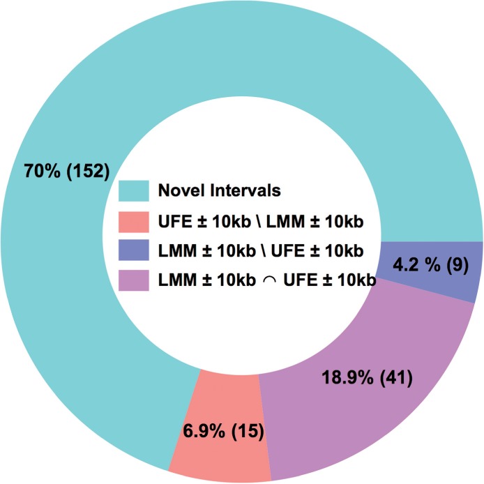
Proportion of novel intervals among all intervals found by FAIS-WY, across all phenotypes. The green part shows the proportion of novel intervals found by FAIS-WY. The red part (UFE ± 10 kb\LMM ± 10 kb) are intervals containing an UFE hit or are in close proximity (±10 kb) to one and the hit could not be found with a LMM. The blue part (LMM ± 10 kb\UFE ± 10 kb) are intervals containing a LMM hit or are in close proximity (±10 kb) to one and the hit could not be found with an UFE. The purple part (LMM ± 10 kb∩UFE ± 10 kb) are intervals that contain both, a hit (±10 kb) found with an UFE and a LMM

3.3 Biological annotation and interpretation

We used the tool snpEFF (Cingolani et al., 2012) to annotate all genetic variants found in the most significant intervals of FAIS-WY that do not contain a significant hit found by an UFE (Supplementary Table S2)—referred to as noUFE filtering—and that do not contain or are in close proximity to any significant hit found with an UFE or a LMM—referred to as stringent filtering (Supplementary Table S3).

For each of the bacterial pathogenesis factors in our dataset (avrB, avrRpm1, avrPhpB and avrRpt2), the plant receptor that mediates the defense response was previously known (Grant et al., 1995, 1998; Mauricio et al., 2003; Warren et al., 1998; Yu et al., 1993) and had also been detected in previous GWA studies (Aranzana et al., 2005; Atwell et al., 2010). Under the noUFE filtering, the most significant intervals for avrPhpB and avrRpt2 were found in close proximity (<10 kb) to the corresponding R-genes [RESISTANCE TO PSEUDOMONAS SYRINGAE 5 (RPS5) and RESISTANCE TO PSEUDOMONAS SYRINGAE 2 (RPS2), respectively]. The same was true for the lesioning phenotype, where the most significant interval was found just upstream of the known causal gene ACCELERATED CELL DEATH (ACD6) (Todesco et al., 2010). All of these genes are known to have more than one allele that is maintained across different lineages (Stahl et al., 1999; Tian et al., 2002; Todesco et al., 2010). If these alleles arose independently in different genetic backgrounds, individuals that share the same allele would have different nearby polymorphisms. Thus, these intervals of genetic heterogeneity might reflect close linkage to a true causal polymorphism that is maintained by selection in different lineages.

After filtering out intervals that were <10 kb from a previous UFE or LMM hit (stringent filtering), the most significant interval for the avrPhpB was found to be ∼18 kb upstream of RPS5. There is a cluster of genes encoding flavin monooxygenase (FMO) family proteins in this region and a member of this family, FMO1, has previously been shown to be an important regulator of R-gene-mediated defenses (Bartsch et al., 2006). Under these filtering criteria, the most significant interval for avrRpt2 was found in a region nearby two R-genes. For lesioning, the most significant interval encoded a chloroquine resistance transporter, which was previously shown to be important for resistance to Phytophthora brassicae (Maughan et al., 2010).

For all other phenotypes, the most significant interval did not change between the noUFE and stringent filtering. For the avrB phenotype, the most significantly associated interval contained AT3G07195 (Supplementary Tables S2 and S3), a gene that encodes a paralog of the negative immune system regulator RPM1 INTERACTING PROTEIN 4 (RIN4) (Liu et al., 2011; Mackey et al., 2002). This interval was also identified in association with the response to another bacterial pathogenesis factor, avrRpm1 where it was the second-most significant interval. Because both avrB and avrRpm1 are detected by the host immune receptor RESISTANCE TO PSEUDOMONAS SYRINGAE PV MACULICOLA (Rpm1) through modification of RIN4 (Belkhadir et al., 2004; Mackey et al., 2002), it suggests a plausible role for this RIN4 paralog in mediating natural variation in response to the activity of these bacterial virulence determinants.

We also found that two phenotypes that are not related to defense had intervals that contained a cluster of two or more paralogs. In the case of leaf rolling at $10{}^{°}\text{C}$ (Leaf roll 10), the most significant interval covered a cluster of receptor-like proteins. For the lesioning or yellowing phenotype (LY), there was a cluster of RING domain/U-box proteins in the most significant interval. Thus, intervals of genetic heterogeneity may reflect copy number variation or rearrangements that are common features of paralog clusters (reviewed in Żmieńko et al. 2014).

For other phenotypes, the polymorphisms in the interval itself may have a role in explaining the phenotype. The most significant intervals for two of the phenotypes that indicated reduced chloroplast function (YEL and Chlorosis 22) contained a gene that encoded a protein that was predicted to be localized to the chloroplast.

Taken together, these results suggest that intervals of genetic heterogeneity associated with biological traits may result from (i) linkage to an allele that is maintained independently in different lineages, (ii) structural variation in the region or (iii) true genetic heterogeneity within a gene that is responsible for the phenotype.

4 Discussion and conclusion

We have presented an algorithm for detecting genomic intervals of SNPs that may jointly explain the genetic heterogeneity underlying a phenotype of interest. On data from Arabidopsis thaliana, we discover novel genomic regions that may be involved in the genetic heterogeneity of several defense and developmental phenotypes.

Our method improves the state of the art in two important ways: First, it automatically finds the starting and ending positions of these intervals in the genome, while current approaches require the definition of a fixed starting and ending point for each interval. Second, despite the huge number of intervals that we are testing, we can properly account for the resulting problem of multiple hypothesis testing without losing statistical power, that is the ability to detect true intervals. Hence, our algorithm combines in a unique way the ability to efficiently mine the genome for intervals of genetic heterogeneity with a proper way to measure the statistical significance of our findings.

Our method is based on a number of assumptions, which should be overcome in future work in order to further extend the applicability of our method. First, we do not model confounders such as population structure. That is, we do not account for the fact that there may be distinct subpopulations of individuals in our sample (Lippert et al., 2011). We envision extending our method in this direction by conducting meta-analyses, that is searching significant intervals in different subpopulations and then combining these results, e.g. via the Cochran–Mantel–Haenszel test (Mantel and Haenszel, 1959), while still accounting for multiple testing. Second, the method is encoding-sensitive in the sense that changing the binary encoding of a particular SNP will affect the results, and potentially lead to an interval being missed. As in many multi-locus interaction models (e.g. Kam-Thong et al., 2012), it is an open problem how to overcome this coding-sensitivity, while retaining the computational efficiency and statistical power of our current method.

Third, we here consider contiguous intervals of SNPs that exhibit genetic heterogeneity, rather than arbitrary sets of SNPs anywhere in the genome. This decision is based on the computational and statistical consideration that the number of candidate sets is quadratic in the number of SNPs in our setting, but exponential in the size of the candidate sets in the general setting. Still, it is an important question to ask whether our approach here can be extended to detect groups of SNPs in gene pathways (Wang et al., 2010) that may explain the genetic heterogeneity of a given phenotype.

Based on our results, we propose three reasons that explain why an interval of genetic heterogeneity is associated with a phenotype. First, regions flanking a locus that is under balancing selection exhibit polymorphisms that are linked to the segregating alleles (Hudson and Kaplan, 1988) and this can give rise to genetic heterogeneity that is associated with a phenotype that is governed by the locus under selection. All three of the R-genes (Rpm1, Rps5 and Rps2) that govern the responses to the four bacterial pathogenesis factors (avrB, avrRpm1, avrPhpB and avrRpt2) in our phenotype dataset were previously found to be under balancing selection (Mauricio et al., 2003; Stahl et al., 1999; Tian et al., 2002). We found that at least one of the significant intervals of genetic heterogeneity for each of these bacterial pathogenesis factor phenotypes was in the region flanking the corresponding R-gene (Supplementary Table S2). Because all of these phenotypes also had a hit in previous UFE test or LMM GWAS for the cognate R-gene, these intervals were filtered out under the no UFE criteria. The same was true for the lesioning phenotype, where the most significant interval that did not contain a significant hit found by an UFE was near the causal ACD6 locus, which is also thought to be under balancing selection (Todesco et al., 2010). Thus, it is possible that intervals of genetic heterogeneity that we detected for other phenotypes in our dataset may also have resulted from linkage to a locus under balancing selection that was previously missed by a univariate or LMM approach.

Second, regions such as multi-copy gene clusters undergo frequent structural rearrangements (McHale et al., 2012) that might become associated with different polymorphisms. Under the most stringent filtering criteria, we found that the most significant interval for four phenotypes (avrPhpB, avrRpt2, LY and Leaf roll 10) overlapped or was adjacent to a multi-copy gene cluster. Therefore, intervals of genetic heterogeneity may reflect structural variation that is missed by single SNP GWAS.

Third, genetic heterogeneity may arise within a gene that underlies a phenotype. Our analysis uncovered a potential role for a RIN4 paralog in determining resistance to the bacterial pathogenesis factors avrB and avrRpm1, but not for avrRpt2 or avrPphB. The host immune receptor Rpm1 recognizes avrB and avrRpm1 (Belkhadir et al., 2004; Mackey et al., 2002), avrRpt2 is detected by another receptor (Rps2) (Axtell and Staskawicz, 2003) and avrPphB is perceived by a third receptor, Rps5 (Shao et al., 2003). All of these interactions are indirect and the virulence factors are not themselves directly recognized by the receptors, but detected through their modifications of targeted host proteins according to the Guard Hypothesis (Jones and Dangl, 2006). For avrB, avrRpm1 and avrRpt2, the target host protein (guardee) is RIN4, while avrPphB targets the unrelated host protein PBS (Shao et al., 2003). The fact that we detected a RIN4 ortholog in a novel interval for responses to two of the three pathogenesis factors targeting RIN4 suggests the intriguing possibility of natural variation in a guardee contributing to pathogen resistance, similar to what has been observed for the tomato guardee RCR3 (Hörger et al., 2012).

In short, we see exciting challenges for future work, but also high potential for the method present here to help in the discovery of genetic heterogeneity at a genome-wide level.

Funding

This work was funded in part by the Alfried Krupp von Bohlen und Halbach-Stiftung (KB), the SNSF Starting Grant ‘Significant Pattern Mining’ (KB), the Max Planck Society (BR), a Grant-in-Aid for Scientific Research (Research Activity Start-up) 26880013 (MS) and the Marie Curie Initial Training Network MLPM2012, Grant No. 316861 (FLL, KB).

Conflict of Interest: none declared.

References

- Aranzana M.J., et al. (2005) Genome-wide association mapping in Arabidopsis identifies previously known flowering time and pathogen resistance genes. PLoS Genet., 1, e60. [DOI] [PMC free article] [PubMed] [Google Scholar]
- Atwell S., et al. (2010) Genome-wide association study of 107 phenotypes in Arabidopsis thaliana inbred lines. Nature, 465, 627–631. [DOI] [PMC free article] [PubMed] [Google Scholar]
- Axtell M.J., Staskawicz B.J. (2003) Initiation of RPS2-specified disease resistance in Arabidopsis is coupled to the AvrRpt2-directed elimination of RIN4. Cell, 112, 369–377. [DOI] [PubMed] [Google Scholar]
- Bartsch M., et al. (2006) Salicylic acid–independent ENHANCED DISEASE SUSCEPTIBILITY1 signaling in Arabidopsis immunity and cell death is regulated by the monooxygenase FMO1 and the nudix hydrolase NUDT7. Plant Cell, 18, 1038–1051. [DOI] [PMC free article] [PubMed] [Google Scholar]
- Belkhadir Y., et al. (2004) Arabidopsis RIN4 negatively regulates disease resistance mediated by RPS2 and RPM1 downstream or independent of the NDR1 signal modulator and is not required for the virulence functions of bacterial type III effectors AvrRpt2 or AvrRpm1. Plant Cell, 16, 2822–2835. [DOI] [PMC free article] [PubMed] [Google Scholar]
- Bonferroni C.E. (1936) Teoria statistica delle classi e calcolo delle probabilità. Pubblicazioni del R Istituto Superiore di Scienze Economiche e Commerciali di Firenze, 8, 3–62. [Google Scholar]
- Burrell R.A., et al. (2013) The causes and consequences of genetic heterogeneity in cancer evolution. Nature, 501, 338–345. [DOI] [PubMed] [Google Scholar]
- Cingolani P., et al. (2012) A program for annotating and predicting the effects of single nucleotide polymorphisms, SnpEff: SNPs in the genome of drosophila melanogaster strain w1118; iso-2; iso-3. Fly, 6, 80–92. [DOI] [PMC free article] [PubMed] [Google Scholar]
- Fisher R.A. (1922) On the interpretation of from contingency tables, and the calculation of P. J. R. Stat. Soc., 85, 87–94. [Google Scholar]
- Grant M.R., et al. (1995) Structure of the Arabidopsis RPM1 gene enabling dual specificity disease resistance. Science, 269, 843–846. [DOI] [PubMed] [Google Scholar]
- Grant M.R., et al. (1998) Independent deletions of a pathogen-resistancegene in Brassica and Arabidopsis. Proc. Natl. Acad. Sci., 95, 15843–15848. [DOI] [PMC free article] [PubMed] [Google Scholar]
- Grimm D., et al. (2012) easyGWAS: an integrated interspecies platform for performing genome-wide association studies. arXiv:1212.4788. [Google Scholar]
- Hayes B.J., et al. (2009) Increased accuracy of artificial selection by using the realized relationship matrix. Genetics Res., 91, 47–60. [DOI] [PubMed] [Google Scholar]
- Hörger A.C., et al. (2012) Balancing selection at the tomato RCR3 guardee gene family maintains variation in strength of pathogen defense. PLoS Genet., 8, e1002813. [DOI] [PMC free article] [PubMed] [Google Scholar]
- Hudson R.R., Kaplan N.L. (1988) The coalescent process in models with selection and recombination. Genetics, 120, 831–840. [DOI] [PMC free article] [PubMed] [Google Scholar]
- Jones J.D., Dangl J.L. (2006) The plant immune system. Nature, 444, 323–329. [DOI] [PubMed] [Google Scholar]
- Kam-Thong T., et al. (2012) GLIDE: GPU-based linear regression for detection of epistasis. Human Hered., 73, 220–236. [DOI] [PubMed] [Google Scholar]
- Kim S., et al. (2007) Recombination and linkage disequilibrium in Arabidopsis thaliana. Nat. Genet., 39, 1151–1155. [DOI] [PubMed] [Google Scholar]
- Kim S., et al. (2009) A multivariate regression approach to association analysis of a quantitative trait network. Bioinformatics, 25, i204–i212. [DOI] [PMC free article] [PubMed] [Google Scholar]
- Lippert C., et al. (2011) FaST linear mixed models for genome-wide association studies. Nat. Methods, 8, 833–835. [DOI] [PubMed] [Google Scholar]
- Liu J., et al. (2011) A receptor-like cytoplasmic kinase phosphorylates the host target RIN4, leading to the activation of a plant innate immune receptor. Cell Host Microbe, 9, 137–146. [DOI] [PMC free article] [PubMed] [Google Scholar]
- Mackey D., et al. (2002) RIN4 interacts with Pseudomonas syringae type III effector molecules and is required for RPM1-mediated resistance in Arabidopsis. Cell, 108, 743–754. [DOI] [PubMed] [Google Scholar]
- Mantel N., Haenszel W. (1959) Statistical aspects of the analysis of data from retrospective studies of disease. J. Natl. Cancer Inst., 22, 719. [PubMed] [Google Scholar]
- Maughan S.C., et al. (2010) Plant homologs of the Plasmodium falciparum chloroquine-resistance transporter, Pf CRT, are required for glutathione homeostasis and stress responses. Proc. Natl. Acad. Sci., 200913689, 107, 2331–2336. [DOI] [PMC free article] [PubMed] [Google Scholar]
- Mauricio R., et al. (2003) Natural selection for polymorphism in the disease resistance gene Rps2 of Arabidopsis thaliana. Genetics, 163, 735–746. [DOI] [PMC free article] [PubMed] [Google Scholar]
- McClellan J., King M.-C. (2010) Genetic heterogeneity in human disease. Cell, 141, 210–217. [DOI] [PubMed] [Google Scholar]
- McHale L.K., et al. (2012) Structural variants in the soybean genome localize to clusters of biotic stress-response genes. Plant Physiol., 159, 1295–1308. [DOI] [PMC free article] [PubMed] [Google Scholar]
- Minato S., et al. (2014) A Fast Method of Statistical Assessment for Combinatorial Hypotheses Based on Frequent Itemset Enumeration. In ECMLPKDD pp. 422–436. [Google Scholar]
- Neale B.M., Sham P.C. (2004) The future of association studies: gene-based analysis and replication. Am. J. Hum. Genet., 75, 353–362. [DOI] [PMC free article] [PubMed] [Google Scholar]
- Pearson K. (1900) On the criterion that a given system of deviations from the probable in the case of a correlated system of variables is such that it can reasonable be supposed to have arisen from random sampling. Philos. Mag., 50, 157–175. [Google Scholar]
- Shao F., et al. (2003) Cleavage of Arabidopsis PBS1 by a bacterial type III effector. Science, 301, 1230–1233. [DOI] [PubMed] [Google Scholar]
- Stahl E.A., et al. (1999) Dynamics of disease resistance polymorphism at the Rpm1 locus of Arabidopsis. Nature, 400, 667–671. [DOI] [PubMed] [Google Scholar]
- Sugiyama M., et al. (2015) Significant subgraph mining with multiple testing correction. In: SIAM SDM, pp. 37–45. [Google Scholar]
- Tarone R.E. (1990) A modified bonferroni method for discrete data. Biometrics, 46, 515–522. [PubMed] [Google Scholar]
- Terada A., et al. (2013) Statistical significance of combinatorial regulations. Proc. Natl. Acad. Sci., 110, 12996–13001. [DOI] [PMC free article] [PubMed] [Google Scholar]
- Tian D., et al. (2002) Signature of balancing selection in Arabidopsis. Proc. Natl. Acad. Sci., 99, 11525–11530. [DOI] [PMC free article] [PubMed] [Google Scholar]
- Todesco M., et al. (2010) Natural allelic variation underlying a major fitness trade-off in Arabidopsis thaliana. Nature, 465, 632–636. [DOI] [PMC free article] [PubMed] [Google Scholar]
- Wang K., et al. (2010) Analysing biological pathways in genome-wide association studies. Nat. Rev. Genet., 11, 843–854. [DOI] [PubMed] [Google Scholar]
- Warren R.F., et al. (1998) A mutation within the leucine-rich repeat domain of the arabidopsis disease resistance gene RPS5 partially suppresses multiple bacterial and downy mildew resistance genes. Plant Cell, 10, 1439–1452. [DOI] [PMC free article] [PubMed] [Google Scholar]
- Wellcome Trust Case Control Consortium. (2007) Genome-wide association study of 14,000 cases of seven common diseases and 3,000 shared controls. Nature, 447, 661–678. [DOI] [PMC free article] [PubMed] [Google Scholar]
- Westfall P., Young S.S. (1993) Resampling-Based Multiple Testing: Examples and Methods for p-Value Adjustment . Wiley, New York. [Google Scholar]
- Yu G.-L., et al. (1993) Arabidopsis mutations at the RPS2 locus result in loss of resistance to Pseudomonas syringae strains expressing the avirulence gene avrRpt2. Mol. Plant Microbe Interact., 6, 434–434. [DOI] [PubMed] [Google Scholar]
- Żmieńko A., et al. (2014) Copy number polymorphism in plant genomes. Theor. Appl. Genet., 127, 1–18. [DOI] [PMC free article] [PubMed] [Google Scholar]
Associated Data
This section collects any data citations, data availability statements, or supplementary materials included in this article.