Toxicokinetic Triage for Environmental Chemicals

Abstract

Toxicokinetic (TK) models link administered doses to plasma, blood, and tissue concentrations. High-throughput TK (HTTK) performs in vitro to in vivo extrapolation to predict TK from rapid in vitro measurements and chemical structure-based properties. A significant toxicological application of HTTK has been “reverse dosimetry,” in which bioactive concentrations from in vitro screening studies are converted into in vivo doses (mg/kg BW/day). These doses are predicted to produce steady-state plasma concentrations that are equivalent to in vitro bioactive concentrations. In this study, we evaluate the impact of the approximations and assumptions necessary for reverse dosimetry and develop methods to determine whether HTTK tools are appropriate or may lead to false conclusions for a particular chemical. Based on literature in vivo data for 87 chemicals, we identified specific properties (eg, in vitro HTTK data, physico-chemical descriptors, and predicted transporter affinities) that correlate with poor HTTK predictive ability. For 271 chemicals we developed a generic HT physiologically based TK (HTPBTK) model that predicts non-steady-state chemical concentration time-courses for a variety of exposure scenarios. We used this HTPBTK model to find that assumptions previously used for reverse dosimetry are usually appropriate, except most notably for highly bioaccumulative compounds. For the thousands of man-made chemicals in the environment that currently have no TK data, we propose a 4-element framework for chemical TK triage that can group chemicals into 7 different categories associated with varying levels of confidence in HTTK predictions. For 349 chemicals with literature HTTK data, we differentiated those chemicals for which HTTK approaches are likely to be sufficient, from those that may require additional data.

Of the 30 000 chemicals that are estimated to be in wide commercial use, only a small subset has been characterized as to their potential toxicological effects in humans or wildlife (Judson et al., 2008; National Research Council, 1984; USGAO, 2013). High-throughput screening (HTS) using in vitro assays, eg, the ToxCast and Tox21 programs, has been proposed as one approach to fill these data gaps by analyzing the activity of these chemicals across a broad range of potential biological targets (Bucher, 2008; Judson et al., 2010). One challenge associated with the interpretation of the HTS data has been relating in vitro bioactive concentrations with relevant in vivo dose values, and doing so on a scale and throughput required to address the large number of chemicals (Judson et al., 2011; Rotroff et al., 2010; Thomas et al., 2013; Tonnelier et al., 2012; Wambaugh et al., 2013, 2014; Wetmore et al., 2012).

For pharmaceutical compounds, in vitro to in vivo extrapolation (IVIVE) methods have been developed to parameterize toxicokinetic (TK) models that relate blood and tissue concentrations to therapeutic doses for clinical studies. The IVIVE methods typically include limited in vitro measurements of hepatic clearance, plasma protein binding, and chemical structure-derived predictions of tissue partitioning (Jamei et al., 2009; Lukacova et al., 2009). The IVIVE methods and resulting TK models are considered effective since the predicted concentrations are often (Wang, 2010) within ∼3-fold of the in vivo observations (we describe predictions as being “on the order of magnitude” if they are within $\sqrt{10}\approx 3.2\text{-fold}$). Ultimately, the human TK of a pharmaceutical compound may be fully characterized in follow-on human clinical trials (Jamei et al., 2009), which is vastly different from the data available for environmental and industrial chemicals where both ethical and cost considerations preclude human testing.

The IVIVE methods developed for pharmaceuticals have been used to parameterize high-throughput TK (HTTK) models for hundreds of environmental and industrial chemicals (Rotroff et al., 2010; Tonnelier et al., 2012; Wetmore et al., 2012, 2013, 2014). The primary example of the application of HTTK models has been to estimate the doses (mg/kg BW/day) needed to produce steady-state plasma concentrations (C_ss, in units of µM) equivalent to concentrations that produce bioactivity in in vitro assays—this process is often described as “reverse dosimetry” (Rotroff et al., 2010; Tonnelier et al., 2012; Wetmore et al., 2012, 2013, 2014). Reverse dosimetry with HTTK models can provide estimated doses for environmental and industrial chemicals below which significant in vitro bioactivity is not expected to occur (Judson et al., 2011; Wetmore et al., 2012). The ratio between the lowest bioactive dose and the maximal expected exposure provides risk-based context to HTS data and is one metric for prioritization of additional chemical testing (Judson et al., 2011; Thomas et al., 2013; Wetmore et al., 2012).

When benchmarked against a limited number of environmental, pesticidal, and industrial chemicals with in vivo TK data, HTTK models have demonstrated mixed success, but have generally provided health-protective estimates of bioactive doses (Wetmore et al., 2012; Yoon et al., 2014). The reasons for the discrepancies between steady-state concentrations predicted using HTTK and the concentrations from in vivo TK data are not clear. There may be extrapolation issues for environmental chemicals that are not present with pharmaceuticals.

This study evaluated the accuracy of HTTK predictions that were made using the same physiologically motivated, 3-compartment mathematical TK model previously used in reverse dosimetry studies (Rotroff et al., 2010; Tonnelier et al., 2012; Wetmore et al., 2012, 2013, 2014). This assessment was conducted across the 349 chemicals for which the appropriate inputs and data were available. Of these, ∼80% of the chemicals (ie, 271), possessed required inputs to parameterize a generic high-throughput physiologically based toxicokinetic (HTPBTK) mathematical model that we employed to test some of the assumptions used in the HTTK-based reverse dosimetry approach for environmental chemicals. HTTK model predictions were further evaluated using available human and rat in vivo measurements curated from TK literature.

We found that some properties of pharmaceutical and environmental chemicals correlated with either small or large discrepancies between HTTK predictions and in vivo-derived values. Those properties define a “domain of applicability” of chemical property space within which HTTK models may be expected to provide an adequate alternative to more traditional TK methods for reverse dosimetry and other applications. The results of our analyses were integrated into a multi-element TK triage system that organizes chemicals into different categories based on varying degrees of accuracy (eg, on the order, 10× over-estimated, 10× underestimated) of the HTTK predictions with additional categories for situations where more data or alternative approaches are needed to develop suitable TK models. Depending on the accuracy needed for a specific application and the degree of confidence for a particular prediction, this triage system separates those chemicals with which HTTK may be used with confidence from those chemicals that may benefit from specific types of analyses and/or additional experimental data collection.

MATERIALS AND METHODS

In this study, we first replicated the steady-state TK model used in previous studies and developed a new model allowing exploration of the impact of the steady-state assumption. We used these models to analyze the soundness of assumptions used in previous reverse dosimetry HTTK applications as exemplified by the Wetmore et al. (2012) study. We then applied statistical methods to determine the chemical-specific properties that correlate with HTTK predictive ability. Among the chemical-specific properties examined, we investigated xenobiotic transporter affinities predicted using quantitative structure–activity relationships (QSAR). The methods and data used for our analysis of HTTK have been made available as a package for the open source R statistical analysis software platform (R Development Core Team, 2013). The package, “httk,” can be accessed from the Comprehensive R Archive Network (CRAN) repository (http://cran.r-roject.org/web/packages/httk/, last accessed 22 June 2015). All chemical-specific parameters are listed in Supplementary Table 1 with references.

TK models used

Two general (ie, chemical independent) TK models were used. The first model was intended to replicate the model used in previous reverse dosimetry analyses (Rotroff et al., 2010; Wetmore et al., 2012, 2013). Those analyses were performed using the SimCyp software (Jamei et al., 2009). The first model (illustrated in Supplementary Fig. 1) was a physiologically motivated “3-compartment” model for determining plasma concentrations that assumed no tissue partitioning, elimination due to metabolism of the parent compound in the liver, renal elimination by passive glomerular filtration (GF), and is adjusted for plasma protein binding [ie, GF rate (GFR) × fraction of chemical unbound in plasma]. Metabolism in this model is comparable to the “well-stirred” approximation for hepatic metabolism (Wilkinson and Shand, 1975).

The second general TK model (illustrated in Supplementary Fig. 2) was physiologically based (PBTK) with separate tissue compartments for the gut, liver, lung (unused for dosing in this research, since the inhalation route was not simulated), kidneys, and arterial and venous blood. The rest of the tissues in the body were aggregated. Tissue volumes and blood flows were taken from Birnbaum et al. (1994). Tissue flows and volumes were scaled to cardiac output and body weights from Davies and Morris (1993), which also provided values for GFR and hematocrit. Absorption from the gut lumen into gut tissue was modeled as a first-order process with an arbitrary, “fast” rate of 1/h. Venous blood from the gut and arterial blood fed separately into the liver, where metabolism was again modeled with the “well-stirred” approximation.

Physico-chemical and partitioning information were collated from various sources. Molecular weight and structure were determined from the DSStox database (http://www.epa.gov/ncct/dsstox, last accessed 22 June 2015) and hydrophobicity was drawn for all compounds from EPI Suite (http://www.epa.gov/opptintr/exposure/pubs/episuite.htm (last accessed 22 June 2015)—measured values used if available, predicted otherwise). Where available, ionization association/dissociation equilibrium constants were curated from the literature; otherwise predictions were based on chemical structure using the SPARC (SPARC Performs Automated Reasoning in Chemistry) model (Hilal et al., 1995). Experimental values for membrane affinities (ie, lipid-bilayer to water concentration ratios) were used where available (Endo et al., 2011) or predicted using a regression of the Endo et al. (2011) data based on hydrophobicity and temperature:

$${\log }_{10}\left(K_{\text{npl:water}}\right)=0.999831-0.016578\times T+0.881721\times {\log }_{10}\left(K_{\text{octanol:water}}\right),$$

where T is the temperature (°C), $K_{\text{npl:water}}$ is the neutral phospholipid-to-water concentration ratio, and $K_{\text{octanol:water}}$ is the octanol-to-water concentration ratio.

Chemical-specific tissue to free fraction in plasma partition coefficients were predicted using Schmitt’s method (2008a). Tissue-specificity was based upon the cellular fraction of total volume; water, lipid and protein fraction of cellular volume; and distribution of types of lipid (Schmitt, 2008b). Chemical-specificity was based upon plasma protein binding (fup), the hydrophobicity, and any ionization association/dissociation constants. Because we do not have a method for estimating the rate at which chemicals diffuse into tissues, we assumed that all tissues were perfusion-limited; ie, chemical concentrations in tissue, red blood cells, and plasma come to equilibrium instantaneously relative to the flow of blood.

Determination of steady state

We use the term “steady-state” to describe the situation where the chemical concentration in plasma caused by the assumed exposure scenario is unchanging in time. With the assumption of constant infusion dosing, as in Wetmore et al. (2012), this is a true steady-state. With constant infusion dosing the flow of chemical into the body is matched perfectly by clearance from the body. For dynamic exposure scenarios (such as exposures separated by time intervals), a quasi-steady-state is determined to occur if the plasma concentration effectively no longer increases across a fixed time interval. For example, if plasma concentration is the same just before the next dose as it was before the current dose, this is quasi-steady-state.

In order to determine if steady-state conditions were achieved, 2 analytic equations were derived from the differential equations of the 3-compartment TK and PBTK models by assuming constant infusion dosing. The analytic solution to the 3-compartment TK model is the equation used for steady-state plasma concentrations (C_ss) in previous work (Rotroff et al., 2010; Wetmore et al., 2012, 2013; Wilkinson and Shand, 1975). For the PBTK model, equations were solved numerically to simulate a series of repeated, every 8-h oral doses until the daily averaged venous concentration, just before re-dosing, was within a small tolerance (1%) of the concentration predicted with the analytical solution of the PBTK model. The PBTK simulations assume an initial body burden of no chemical, even though this may not be the case for certain persistent, bioaccumulating, or endogenous chemicals. The equations for the analytic solutions are given in the captions to Supplementary Figures 1 and 2.

In vitro chemical data

In vitro data used in this study was extracted from published literature. For environmental, pesticidal, and industrial chemicals, in vitro experimental data were obtained primarily from Wetmore et al. (2012) and Tonnelier et al. (2012). For pharmaceutical compounds these values were compiled from Obach (1999), Jones et al. (2002), Shibata et al. (2002), Lau et al. (2002), Naritomi et al. (2003), Ito and Houston (2004), McGinnity et al. (2004), Schmitt (2008a), and Obach et al. (2008).

Two types of in vitro data were extracted in order to parameterize the TK models—intrinsic hepatic clearance and plasma protein binding. The intrinsic metabolic clearance of the parent compound (CL_int) by primary hepatocytes (substrate depletion approach) was measured in wells on a multi-compound plate (Shibata et al., 2002). Since only the unbound chemical in the hepatic clearance assay is available for metabolism, CL_int was determined from the observed clearance (CL_uint) which was divided by the estimated fraction of chemical unbound in the hepatocyte intrinsic clearance assay (f_uhep), as estimated using the method of Kilford et al. (2008). The Kilford et al. (2008) method includes a distribution coefficient estimated from hydrophobicity and ionization. In Wetmore et al. (2012), 2 chemical concentrations (1 and 10 µM) were tested, in part to test for saturation of metabolism. We have used only the 1 µM values. Fraction of chemical unbound in the presence of plasma protein (f_up) was assessed using rapid equilibrium dialysis (RED) in which 2 wells are separated by a membrane that is permeable to smaller molecules but prevents the plasma protein from migrating from one well to the other (ie, the relative chemical concentration in the 2 linked wells gives the free fraction of chemical) (Waters et al., 2008).

Monte Carlo simulation and parameter distributions

Previous reverse dosimetry analyses (Rotroff et al., 2010; Wetmore et al., 2012) used the SimCYP software (Jamei et al., 2009) to perform a Monte Carlo (MC) simulation of human variability and we have implemented a similar MC simulation ability. To match the assumptions used by SimCYP, normal distributions that were truncated to ensure positive values were used with mean values drawn from the references above and a coefficient of variation of 0.3. Body weight, liver volume, hepatic blood flow, glomerular filtration rate, and CL_uint were all varied in this manner. In a change from previous MC simulations, the values for protein binding, f_up, were drawn from a censored normal distribution: values were sampled from a uniform distribution between 0% and the limit of detection (LOD) (default of 1% unbound) at a rate proportional to the number of samples from the truncated normal distribution below the LOD. For each chemical, 1000 different combinations of parameters were used to determine C_ss, allowing estimation of the 5th, median, and 95th percentiles.

In vivo chemical data

In Wetmore et al. (2012), in vivo TK and PBTK modeling data for the environmental, pesticidal, and industrial chemicals were collected from the literature and used to assess the predictive ability of the human in vivo C_ss estimation, assuming a 1 mg/kg/day daily oral administration. For pharmaceutical compounds, the measured human clearance (l/day) and volume of distribution (l) in Obach et al. (2008) was used to determine C_ss for the same dose.

Model compounds for rat IVIVE were chosen based on the availability of HTTK input parameters CL_uint and f_up. A list was constructed from Ito and Houston (2004), complemented by a group of compounds to which reverse dosimetry was applied in earlier studies (Krug et al., 2013; Piersma et al., 2013). For these compounds, we searched public sources for studies reporting plasma concentration time course data in rat following oral or intravenous administration. Pharmacokinetic data were retrieved from those studies (Supplementary Table 2) by digitizing published figures using TechDig v2.0.

In silico transporter predictions

We used the method of Random Forest (Breiman, 2001) to develop QSAR predictions of transporter affinity (Sedykh et al., 2013). We used the R package “randomForest” by Liaw and Weiner (2002). Experimental data characterizing interaction of chemicals with membrane transporters were compiled from multiple available public sources (Sedykh et al., 2013). The chemicals were represented using Chemistry Development Kit descriptors (Steinbeck et al., 2003) determined from Simplified Molecular-Input Line Entry System strings (Weininger, 1988). Chembench (Walker et al., 2010) was used to standardize chemical structures as well as normalize chemical descriptors to range between 0 and 1. Inhibitors were defined based on a potency threshold of 10 μM except for peptide transporter 1 (PepT1), organic cation transporter 1 (OCT1), and organic anion-transporting polypeptide 2B1 (OATP2B1), for which 100 μM threshold was used due to lower levels of affinity of reported inhibitors. Scores equal to 0 or 1 imply high-confidence predictions that a chemical is a non-substrate or a substrate, respectively, whereas a score of 0.5 indicates an ambiguous prediction (Sedykh et al., 2013). The full list of transporters modeled is identified in Supplementary Table 1, which also contains the QSAR predictions for each compound.

A second model, based upon Bayesian classification, was used to predict interactions of the compounds with organic anion transporter protein (OATP) 1B1 (Van de Steeg et al., 2015). The classification model is based on a database recording the inhibitory potential of 640 FDA-approved drugs from a commercial library (10 μM) on the uptake of [3H]-estradiol-17beta-d-glucuronide (1 μM) in Human Embryonic Kidney 293 cells stably transfected with human OATP1B1. The structural similarity (feature-connectivity bit string 4) to the nearest similar chemical in this training set is used as a measure for potential interaction with OATP1B1. Although this model predicts inhibition of OATP1B1-mediated uptake rather than uptake itself, we assume here that the inhibition is mostly competitive and therefore identifies potential transporter substrates.

HTTK-in vivo discrepancy analysis

The Random Forest algorithm was used to analyze the correlation of chemical descriptors with the discrepancy between HTTK predictions and results based on in vivo data. The Random Forest method is cross validated (Breiman, 2001), performing multiple analyses based on different subsets of chemicals and different subsets of chemical descriptors. Fifty thousand regression trees were constructed using random subsets of the data, with a subset of 17 factors considered at each split in the tree, and a minimum terminal node size of 5. Performance of each regression tree was evaluated against the chemicals not used to build that tree. The most important factors in the random forest model were calculated using the method of decrease in node impurities (essentially, a leave 1 factor out method) (Archer and Kimes, 2008). We used the R package “rpart” by Therneau et al. (2014) to perform the method of recursive partitioning (Breiman et al., 1984) to develop a regression tree for the full dataset (ie, not cross-validated). Finally, a random forests approach was used to construct a classifier tree for 5 exclusive categories (“on the order,” “3.2× under-predicted,” “10× under-predicted,” “3.2×over-predicted,” “10× over-predicted”), with a subset of 17 factors considered at each split, and a minimum terminal node size of 1.

RESULTS

Our HTTK models require chemical-specific data on CL_int and f_up to predict human C_ss. We obtained data from the peer-reviewed literature for a total of 349 chemicals. These chemicals include (non-uniquely) 312 Tox21 chemicals, 248 ToxCast chemicals, 74 pharmaceuticals, and 35 chemicals for which human exposure is monitored by the Centers for Disease Control National Health and Nutrition Examination Survey (CDC, 2012). The distribution of the non-zero values of the CL_int and f_up data is roughly log-normal and is similar across the curated literature (Supplementary Figs. 3 and 4).

Figure 1 illustrates our ability to reproduce the Wetmore et al. (2012) results. As in Wetmore et al. (2012), we simulated population variability to determine the median, lower 5th, and upper 95th percentile of plasma concentrations for individuals exposed to the same, fixed dose (1 mg/kg BW/day). Since the upper 95th percentile individuals have higher plasma concentrations for the same exposure, they are considered to be an example of a sensitive population. Any 1 chemical in Figure 1 is indicated by 3 plot points connected by a line. The 3 points correspond to the median, lower 5th, and upper 95th percentiles of the C_ss. The dashed line indicates the identity (perfect predictor) line—the further a prediction is from the identity line the greater the discrepancy. We describe predictions with large discrepancies as “outliers.”

FIG. 1.

Comparison of the median, upper, and lower 95th healthy adult human percentiles of steady-state plasma concentration (C_ss) predicted on the y-axis using SimCyp (Wetmore et al., 2012) and on the x-axis using assumptions refined to better reflect screening for environmental chemicals. The C_ss values were estimated assuming a steady-state infusion of 1 mg/kg BW/day. Each chemical’s median and upper and lower 95th percentiles are connected by a line. The dashed line indicates the identity (perfect predictor) line.

There was good agreement (R²= 0.84) between our simulations and those in Wetmore et al. (2012) for all 3 percentiles. However, this comparison did identify 2 groups of outliers for which the predictions differ due to differing assumptions.

The first group of chemicals in Figure 1 with differing predictions is those that have an upper 95th percentile C_ss that was significantly higher than previously estimated, though the median and lower percentile values were unchanged. These chemicals are indicated in Figure 1 by a bent line connecting the 3 quantiles. This predicted difference indicates greater risk for the most sensitive individuals. This difference was due to replacing a default value with a censored distribution for chemicals with a failed RED assay for measuring f_up (protein binding). Among other reasons (eg, binding to membrane), the RED assay can fail because the amount of free chemical is below the LOD. In Wetmore et al. (2012), the RED assay failed for ∼38% of the chemicals. For these chemicals, Wetmore et al. (2012) assumed a default value of 0.5% free (roughly half the average LODs). For the analysis shown in Figure 1, we have replaced this default value with a censored distribution in our MC variability simulation (essentially, simulating many different values between 0 and 1%).

There was a second group of chemicals in Figure 1 where the current modeling provided plasma concentration estimates different from Wetmore et al. (2012) due to a change in assumptions. This group contained chemicals where differences in the analysis of the hepatic clearance assay results led to different concentrations predicted for all 3 population percentiles in Figure 1 (ie, 3 quantiles connected by a line that are all distant from the identity line). Due to measurement variability and other factors, a linear model may not describe the decrease in parent chemical concentration as a function of time. Previously, a P-value threshold of .10 (probability of the null hypothesis of no disappearance of chemical was <10%) was used to determine if the chemical showed significant intrinsic clearance over the time examined. For the results shown in Figure 1, we have required that P-values be <.05. For those with a P-value >.05, we use a default value of 0 (ie, no hepatic clearance) which acts to increase the estimated plasma concentration for a fixed dose.

Most discrepancies between our predictions and Wetmore et al. (2012) disappear (R²∼ 0.90, Supplementary Fig. 5) if we replace our revised assumptions with the original assumptions of Wetmore et al. (2012). However, 8 discrepant chemicals remain due to issues such as the only C_ss available in Wetmore et al. (2012) was calculated using the 10 µM clearance data. The lone chemical for which we under-predict the value from Wetmore et al. (2012) for all 3 population percentiles is Chlorpyrifos-methyl, for which the 10 µM clearance assay was not statistically significant, leading Wetmore et al. (2012) to use 0 clearance. Since the clearance assays conducted at 1 µM was statistically significant, we used that value, leading to a larger predicted clearance.

Once we were satisfied that we could reproduce previous results for the majority of chemicals, and understood those cases where we differed, we proceeded to evaluate 3 key assumptions for the calculation of C_ss. Previously, chemical partitioning into tissues (eg, volume of distribution) was not determined from HTTK data, necessitating the use of C_ss as a dose metric because the concentration at steady-state does not depend on the amount of chemical in tissues. This means that we assume that humans reach steady state with respect to environmental exposures. Using the analytic solution for C_ss requires the further assumption of constant infusion dosing. Constant infusion dosing requires that we assume that steady-state plasma concentrations are a reasonable surrogate for peak concentrations which would be caused by other exposure scenarios (eg, exposure at meal times only). Further, constant infusion dosing requires either the assumption that 100% of the chemical is absorbed or the use of additional models to predict absorption. Wetmore et al. (2012) selected 100% absorption as being conservative (causing overestimated plasma concentration). By constructing non-steady-state, PBTK models, we can assess the plausibility of these 3 assumptions.

We developed HTPBTK models using Schmitt’s method for tissue partitioning (Schmitt, 2008a). We used a generic PBTK model structure that could be parameterized for any chemical using CL_int and f_up and experimental or QSAR-derived physico-chemical properties. Schmitt’s method requires a value for protein binding in order to make predictions; therefore, we could only build HTPBTK models for 271 chemicals. Further assumptions about chemical absorption and bioavailability (ie, rapid absorption and 100% bioavailability) were required in order to parameterize the HTPBTK models.

Figure 2 illustrates our evaluation of the HTPBTK model predictions by comparison to literature in vivo time course data in rats for 22 chemicals. For a given chemical, the specific TK properties, dose, and route of administration result in different plasma concentration kinetics that we have summarized by the time-integrated plasma concentration (Area Under the Curve, AUC). Neglecting route of administration, we find that HTPBTK is predictive (R²= 0.68) of in vivo data (Fig. 2A). When we estimate a difference between oral exposures (which are subject to absorption and bioavailability) and intravenous and subcutaneous dose routes (which are not), we find slightly greater predictive ability (R²= 0.73). We systematically over-predict AUC for chemicals administered orally. The average difference between oral and intravenous doses is 6.4 (95% confidence interval 2.3–18), ie, on average AUCs from oral doses are roughly 6 times lower than predicted. This result indicates that the absorption assumptions we used for HTPBPTK are conservative and health protective since they produce higher predicted exposures. In Figure 2B, we show that peak plasma concentration (C_max) also appears to be well described by the HTPBTK model (R²∼ 0.68) and that there is a systematic bias toward over-prediction. The treatments that are over-estimated are predominantly for intravenous doses while predictions for oral doses are more evenly scattered about the identity line. The handful of cases where HTPBTK under-predicts C_max are all for oral administration.

FIG. 2.

Evaluation of the predictive ability of HTPBTK models by comparing predictions with in vivo measurements in the rat for the AUC (A) and C_max (B). Each chemical may have more than one study with potentially different doses and routes. Dose route is indicated by symbols (oral, po—triangle; intravenous, iv—circle; subcutaneous, sc – square). The upper dotted line is the linear regression for intravenous doses, while the lower dotted line is for the oral doses. The dashed line indicates the identity (perfect predictor) line.

Having established that our HTPBTK model predictions are consistent with the in vivo data that was available for 22 chemicals (Fig. 2), we conducted a simulation study to evaluate the assumptions used to calculate C_ss in previous HTTK reverse dosimetry analyses. In the simulation study, we replaced the infusion dose assumption with a dosing scenario of 3 daily doses totaling 1 mg/kg BW/day (eg, exposure at meal times or from consumer product use), to better reflect the near field sources of exposure that appear to be dominant for environmental chemicals (Wambaugh et al., 2013). As illustrated in Figure 3A, 70% of chemicals (182 of 271) reach steady-state within 28 days, and 90% of chemicals (252 of 271) reach steady-state within 1000 days. However, there were 19 chemicals that required more than 1000 days to reach steady-state (Table 1). TK analyses based upon C_ss are inappropriate for these chemicals, suggesting a need for alternative approaches. Approaches based on dynamic TK simulation of the tissue concentrations likely to be caused over a life-time of exposure may be more appropriate. The 5 chemicals that never reach steady-state (ie, the ratio of the simulated average daily concentration to the analytic C_ss never approaches 1) are polychlorinated biphenyls (PCBs), which are known to have long human half-lives (Ritter et al., 2010) and are no longer deliberately in commerce.

FIG. 3.

HTPBTK simulation results evaluating the steady-state infusion assumption to predict C_ss. A, Histogram of number of chemicals versus the days needed to effectively reach steady-state assuming 3 daily doses (every 8 h). B, Comparison of peak plasma concentrations due to 3 daily does predicted with the HTPBTK model with the C_ss due to a constant infusion exposure as used in Figure 1 and previous reverse dosimetry studies. The dashed line indicates the identity (perfect predictor) line.

TABLE 1.

Chemicals Predicted to Require Long Time Periods to Reach Steady-State

Compound	CAS	Analytic Css (mg/l)	HTPBTK Average Daily Conc. (mg/l)	Ratio of HTPBTK to Analytic After 100 Years	Years to Steady-State	Vd (l)	Kel (h)
Fenpropathrin	39515-41-8	0.36	0.36	0.99	3.0	651.3	0.000162
Perfluorooctanoic acid	335-67-1	81.55	81.39	0.99	3.5	3.4	0.00015
Imazalil	35554-44-0	13.37	13.17	0.99	4.1	24.8	0.000128
Maprotinline	10262-69-8	0.8	0.8	0.99	4.9	480.9	0.000106
Tetraconazole	112281-77-3	15.92	15.67	0.99	5.7	28.9	9.22E−05
Perfluorooctane sulfonic acid	1763-23-1	81.83	81.66	0.99	6.6	6.4	7.92E−05
Isoxaben	82558-50-7	8.4	8.25	0.99	6.8	65.5	7.71E−05
Ddt	50-29-3	0.04	0.04	0.99	7.3	15127.0	3.84E−05
s-bioallethrin	28434-00-6	1.66	1.63	0.99	9.0	434.5	5.85E−05
Fenvalerate	51630-58-1	0.88	0.88	0.99	13.7	1235.3	3.71E−05
Zoxamide	156052-68-5	37.87	37.69	0.99	34.0	71.3	1.55E−05
Oxyfluorfen	42874-03-3	3.21	3.18	0.99	41.7	1033.9	1.26E−05
d-cis, trans-allethrin	584-79-2	1.35	1.33	0.99	46.7	2763.0	1.13E−05
Emamectin benzoate	155569-91-8	282.45	281.50	0.99	77.7	21.8	6.77E−06
PCB136	38411-22-2	37.68	1.08	0.03	>100	34485.6	3.21E−08
PCB153	35065-27-1	76.7	0.86	0.01	>100	43391.9	1.25E−08
PCB155	33979-03-2	75.67	1.36	0.02	>100	27407.8	2.01E−08
PCB77	32598-13-3	76.21	10.56	0.13	>100	3314.2	1.65E−07
PCB80	33284-52-5	77.06	11.26	0.14	>100	3093.6	1.75E−07

With the HTPBTK models and more realistic exposure simulation, we then compared predicted peak concentrations with the C_ss derived from the analytical solution to the 3-compartment TK model (Fig. 1). As shown in Figure 3B, the peak concentration for repeated dosing is not different (R²∼ 0.95) from the C_ss predictions under the assumption of constant infusion dosing. Similarly, the average daily concentration at steady-state was nearly identical (R²∼ 0.96) to the analytical result for C_ss used in Wetmore et al. (2012) and elsewhere (Supplementary Fig. 6). For rapidly cleared compounds, the peak concentrations from 3 daily doses were within an order of magnitude of C_ss.

We then compared HTTK predictions of C_ss based on in vitro data with C_ss values inferred for humans from in vivo studies for 11 environmental chemicals (Wetmore et al., 2012) and 74 pharmaceuticals (Obach et al., 2008). Figure 4A illustrates that there is a weak predictive ability (R²∼ 0.34), but that the errors are mostly conservative (ie, the predicted plasma concentrations based on in vitro data are higher than the in vivo data indicates). When the perfluorinated chemicals (PFCs) are removed, the R² drops to ∼0.23. We note that the correlation between the HTTK C_ss versus the C_ss inferred for humans from in vivo studies is lower than observed for AUC and C_max predictions in Figure 2. At steady-state, all C_ss values are compared for the same fixed dose rate of 1 mg/kg/day. When the HTPBTK predictions are normalized for administered dose, the R² for AUC and C_max drop to ∼0.48 for both, indicating that a portion of the predictive ability of the HTPBTK might be due to the data varying linearly with dose for those chemicals.

FIG. 4.

A, Comparison of HTTK predicted C_ss values with measured in vivo C_ss values from literature studies. Two PFCs are plotted on top of each other. The dashed line indicates the identity (perfect predictor) line. Chemicals plotted below the identity line have predictions greater than literature values, and vice versa. The thick grey lines indicate the discrepancy between measured and predicted values (ie, the residuals). Comparison of the actual residuals calculated from (A) and the residuals predicted using a random forest analysis based on chemical descriptors is shown in (B). The most important factors in the random forest model, as calculated using the method of decrease in node impurities, are shown in (C). These factors are described in detail in Tables 2 and 3.

To identify chemical-specific properties that correlate with reduced HTTK predictive ability, we analyzed the difference between in vivo measurements and HTTK predictions (ie, the residuals), shown by thick grey lines in Figure 4A. The method of random forests was used to predict the residual for each chemical with in vivo data, as shown in Figure 4B. Chemical properties included chemical-specific physico-chemical properties, in vitro intrinsic hepatic clearance, in vitro plasma protein binding, and QSAR predictions of transporter affinity. Transporters were included because predictors were available (Sedykh et al., 2013) and they constitute an often important driver of TK (Giacomini et al., 2010; Shugarts and Benet, 2009) that is not included in the steady-state model. A large predicted residual for a specific chemical corresponds to a large expected error. The random forest approach ensures cross-validated predictive ability by averaging the predictions of many models constructed from random subsets of the chemicals and chemical descriptors. The relative importance of the top 10 chemical properties for predicting HTTK residuals (errors) is illustrated in Figure 4C. These factors are described in detail in Tables 2 and 3. Note that all transporters that were included as potential predictors of error were anticipated to be relevant to TK. The relative rankings of specific transporters in Table 2 may reflect the chemical evaluation set that was used.

TABLE 2.

Transporters Associated With Differences Between HTTK Model Predictions and Human in vivo C_ss

Abbreviation (Gene)	Full Name	Transporter	References	Random Forest Importancea	Included in Tree Made From All Data
BSEP (ABCB11)	Bile Salt Export Pump	Hepatocyte bile secretion efflux transporter	Faber et al. (2003) and Giacomini et al. (2010)	10.3
BCRP (ABCG2)	Breast cancer resistance protein	Hepatocyte bile and intestinal secretion efflux transporter	Giacomini et al. (2010)	9.97
OCT1 (SLC22A1)	Organic Cation Transporter 1	Hepatocyte influx and intestinal secretion influx transporter	Faber et al. (2003) and Giacomini et al. (2010)	6.64
MCT1 (SLC16A1)	Monocarboxylate Transporter 1	Ubiquitous Transporter	Halestrap and Meredith (2004)	6.6	Y
OATP2B1 (SLCO2B1)	Solute carrier organic anion transporter family member 2B1	Hepatocyte and blood-brain barrier influx transporter	Giacomini et al. (2010)	5.77	Y
PEPT1 (SLC15A1)	Peptide transporter 1	Intestinal and kidney secretion influx transporter	Giacomini et al. (2010)	5.54	Y

^aLarger value indicates greater relative importance. When multiple predictors for same transporter were available, only the highest reported importance is reported.

TABLE 3.

Other Factors Associated With Difference Between HTTK Model Predictions and Human in vivo C_ss

Factor	Description	Random Forest Importancea	Included in Tree Made From All Data
fup	Fraction unbound to plasma protein as measured in vitro	51.0	Y
Predicted Css	Steady-state concentration predicted from in vitro measured fub and Clint	43.1	Y
Ionization (pKa_Donor)	Acid dissociation equilibrium constant	20.2
Elimination rate (ke)	Elimination rate as calculated from total clearance (renal + hepatic) predicted from in vitro data, divided by Vd	16.9
Log Kow	Log transformed hydrophobicity (ratio of concentration in octanol to water)	8.86
Perfluorinated compound (PFC) (yes/no)		6.65

^aLarger value indicates greater relative importance.

Although the random forest method produces a cross-validated predictor, the interpretation of how those predictions are achieved can be difficult since the predictions are the average of many different models. A single regression tree for predicting C_ss residuals based on all chemicals and all available chemical properties can be created for descriptive purposes (Fig. 5). Error in the HTTK models (ie, large residuals) appears to be driven by predicted C_ss, f_up, chemical ionization, and 2 of the transporters described in Table 2. We note 2 broad classes of chemicals—those chemicals where HTTK predictions are on the order (ie, within ∼3.2× or 10^1/2×) of the observed in vivo values (∼65% of the chemicals), and those chemicals where the errors can be several orders of magnitude (28% of the chemicals were ∼6× overestimated, and 8% of chemicals 120× overestimated on average). For this final group of chemicals, the large overestimation by the HTTK models leads to conservative reverse dosimetry predictions (ie, errors that would lead to lower predicted ratios between bioactive doses and the maximal expected exposures, thus leading to a higher predicted risk).

FIG. 5.

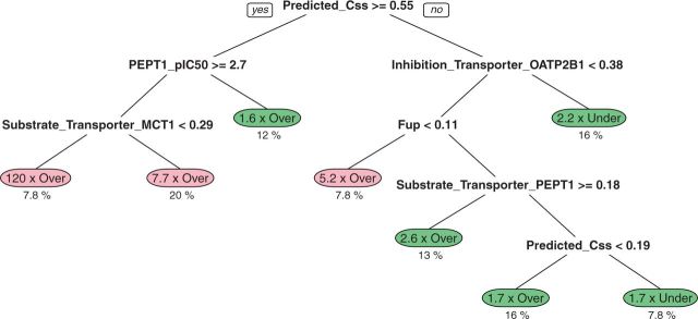
A recursive partitioning regression tree was used to classify the discrepancy between the C_ss predicted from in vitro data and the in vivo C_ss (Obach et al., 2008; Wetmore et al., 2012). Each “leaf” of the tree shows a group of chemicals for which HTTK either overestimates C_ss (making conservative predictions) or underestimates C_ss. For all but 3 groups, the predictions are on the order of the observed C_ss (approximately within a factor of 3.2× greater or lesser). For the other 3 groups, the C_ss is 5.2×, 7.7×, and 120× overestimated. The dashed line indicates the identity (perfect predictor) line.

Motivated by the regression tree analysis in Figure 5, which classified all the data but was not suitable for prediction, a second random forest (ie, predictive, rather than descriptive) analysis was conducted. The analysis used the same descriptors as before to classify chemicals into 5 categories based on residual: those chemicals with predictions on the order of the in vivo C_ss (within ∼3.2×), those that were between ∼3.2× and 10× over or underestimated, and those that were >10× over or underestimated. The cross-validated classifier had a sensitivity of 79%, a specificity of 54%, and a balanced accuracy of 64% when predicting whether or not a HTTK C_ss prediction will be on the order of the in vivo measured C_ss. Chemicals for which the residuals are predicted to be on the order or overestimated are within the domain of applicability of our HTTK approach; ie, we expect to have either small or conservative errors for reverse dosimetry. Along with identifying those chemicals that never reach steady-state (Table 1) and those chemicals for which the plasma protein binding assay failed, the 5 categories from this random forest classifier allow each chemical to be placed into 1 of 7 categories, as illustrated in Figure 6.

FIG. 6.

Distribution of the 349 chemicals with IVIVE data among the triage elements in Table 4. C_ss is not meaningful for the chemicals that do not reach steady-state. Chemicals where the protein binding assay failed cannot easily be categorized since f_up is an important predictor (Table 3) of discrepancy between HTTK C_ss predictions and literature values for C_ss. The remaining chemicals are categorized as likely having HTTK predictions for C_ss that would be overestimated, underestimated, or on the order (±3.2× the in vivo value).

By integrating the various analyses in this study, we developed a TK triage framework that provides guidance on the degree of confidence for a particular prediction and indicates which chemicals may benefit from specific types of analyses or experimental data collection (Table 4). The first step is the collection of basic in vitro TK data that allows a prediction to be made for C_ss. Second, the parameterization of HTPBTK models using physico-chemical properties and predicted partition coefficients, if possible, allows a determination of the plausibility of reaching steady state. Third, chemical properties that are correlated with large deviations between predicted and observed behavior can be used to screen out those chemicals for which HTTK is not expected to perform well. The 4th element of triage addresses those remaining chemicals in greatest need of alternative, perhaps traditional approaches. Different elements of triage may be applied concurrently, depending on the information that is available.

TABLE 4.

Elements of HTTK Triage for Environmental Chemicals

	TK Data	Targeted Chemicals	TK Prediction/Consequence	Confidence	Domain of Applicability
1	In vitro clearance of parent compound by hepatocytes and binding to plasma protein	HTS compounds	Plasma Css from constant infusion exposure	If comparison with predicted exposure indicates large AER then infusion Css should be sufficient	Soluble low volatility (HTS appropriate) compounds
1a	CYP-specific in vitro data (Wetmore et al., 2014)	Chemicals with AER near one for general population	Population variability, life-stage variability	Human variations in CYP expression are well characterized	Same as in 1
2	Physico-chemical properties (measured or QSAR)	All chemicals with successful binding in vitro assay	Prediction of partition coefficients allows HTPBTK steady-state predictions (including time to steady state) for more realistic exposure modeling	If comparison with predicted exposure indicates large AER then HTPBTK should be sufficient (ie, conservative due to 100% absorption)	QSAR-defined (eg, training set, extrapolation methodology)
3	QSARs for likely transporter substrates	All chemicals with successful binding in vitro assay	Assumptions of perfusion-limited tissue partitioning and passive renal excretion by glomerular filtration may be questionable	Can identify those chemicals where the impact is negligible (Fig. 4b)	Chemicals predicted to reach steady state in Tier 2 (Fig. 3a)
3b	Transporter-specific in vitro data	Chemicals indicated by QSAR	Tissue-specific accumulation, active secretion/resorption in kidney	Well characterized for non high-throughput applications	Same as in 3
4	In vivo oral and iv dose TK study, plasma only	Chemicals with large predicted residuals (Fig. 4b) and those that cannot be tested in vitro	Oral bioavailability, absorption rate, volume of distribution, and clearance (refined PBTK model)	If volume of distribution from HTPBTK model and in vitro estimate of clearance hold, then refined PBTK model should be excellent	Any compound

AER is the Activity to Exposure Ratio between HTS bioactive reverse dosimetry predictions and exposure.

We applied the TK triage (Table 4) to the entire 349 chemical set in Figure 6. We find that a plurality (140) of the chemicals are estimated to be “on the order,” ie, the HTTK predicted C_ss will be within ∼3.2× of the literature value. The third largest category is chemicals for which the protein binding assay failed (80), precluding analysis of time to reach steady-state. However, only 7% of chemicals analyzed for time to reach steady-state did not do so within 1000 days, and we might assume this figure to be similar for these 80 chemicals. Of the remaining 110 chemicals, most (102) are predicted to be overestimated, leading to conservative errors when conducting reverse dosimetry. In total, we predict that the reverse dosimetry assumptions will be appropriate for 89% of the chemicals where the protein binding assay was successful.

DISCUSSION

Efforts to implement the vision outlined in Toxicity Testing in the 21st Century (National Research Council, 2007) include in vitro assays to identify potential biological targets of environmental and industrial chemicals (eg, ToxCast, Judson et al., 2010). IVIVE methods are then needed to translate in vitro bioactive concentrations into administered doses (Blaauboer et al., 2012; Wetmore et al., 2012). HTS data might then be used in a risk-based context through the comparison of estimated bioactive doses to estimated exposures (Judson et al., 2011; Thomas et al., 2013; Wetmore et al., 2012). Herein, we develop a method for identifying the degree of confidence with which we may apply HTTK in order translate HTS data for chemicals without other TK data. We have formalized this process in a triage system that has categorized 349 chemicals into 7 categories, 5 of which indicate varying degrees of confidence in the HTTK approach and 2 indicate a need for additional data or alternative approaches.

We examined 3 key assumptions in the previous HTTK research: that humans can reach a steady-state with respect to environmental exposures, that steady-state concentration is a reasonable surrogate when exposure is more episodic, and that 100% absorption is reasonable. These assumptions were tested using both simulation studies and direct comparison to in vivo data for both pharmaceuticals and environmental chemicals. Based on our analysis we organize HTTK testing into a TK triage framework for environmental chemicals (Table 4). Each element of the framework depends on data collection and/or analysis, and distinguishes those chemicals for which that sort of data is useful from those chemicals for which the approach does not apply. Based on this approach we expect the in vivo values to be within ∼3.2× of predictions for ∼59% the 246 chemicals that both had a successful plasma protein binding estimate and we predict will reach steady-state. We expect conservative errors for an additional ∼37% of these 246 chemicals.

The final element of triage incorporates additional in vitro or in vivo testing for those chemicals that are most in need of additional attention. Admittedly, the domain of applicability for this approach is limited by the domain of chemicals used to conduct this analysis. Since there may be chemical properties that drive HTTK error that may be underrepresented by these chemicals, it will also be important to study at least a few members of diverse and novel classes of environmental and industrial chemicals.

The application of in vitro methods to TK is different in the pharmaceutical versus environmental chemical screening domains. For instance, it is expected that some samples of some compounds will be below the LOD of the cost-effective analytical chemistry that is required for the rapid TK screening of thousands of environmental and industrial chemicals (Rousu et al., 2010; Wetmore et al., 2012). When screening environmental and industrial chemicals, resources may not exist for follow-up work and the data must be used as is. This study found that typical assumptions such as half the LOD for protein binding (f_up) (Wetmore et al., 2012) may result in an underestimation of C_ss values, which may not be health protective. However, this may be offset by other assumptions in the HTTK modeling that tend to produce an overestimate of C_ss.

For the metabolic clearance assay, stricter statistical limits are more conservative since they lead to overestimated C_ss values (ie, setting metabolic elimination to 0 for P-value <.05 instead of P-value <.1). However, many of the chemicals that we estimate to have 0 or non-significant clearance in the in vitro assays analyzed here may yield significant clearance in more physiological conditions, such as plated hepatocytes over a longer time period. Follow-up measurement of clearance rates using a plated hepatocytes system (Smith et al., 2012) and/or longer times may ensure a more accurate hepatic clearance estimate.

For most environmental and industrial chemicals it is unlikely that there will ever be controlled human TK data. As evaluated by comparison to in vivo data, the predictive ability of the HTPBTK methods based on both IVIVE and QSAR-related methods was considerably greater than the HTTK models that assumed steady-state conditions. One possible explanation is that although the evaluation data for the HTPBPTK model predictions (in vivo AUCs and C_max values) were drawn from diverse literature, the in vitro data for this comparison were from a single source (Wetmore et al., 2013). For the steady-state HTTK model evaluation, both the in vivo and the in vitro data were drawn from diverse literature sources.

Pharmaceuticals are typically small and well-absorbed molecules that are designed for specific biological targets (Lipinski, 2004). In contrast, environmental and industrial chemicals are structurally heterogeneous and may have multiple biological targets (Richard, 2006). Given the diversity of intended applications for environmental and industrial chemicals, their properties can vary greatly from those of pharmaceuticals. Unfortunately, though in vitro TK data have been collected for many of the 309 ToxCast Phase I chemicals, only 13 in vivo C_ss values were available for those chemicals (Wetmore et al., 2012).

Although the HTPBTK models appear promising for predicting AUC and C_max, the in vivo evaluation data in Figure 2 are drawn from various treatments of only 15 pharmaceutical chemicals and 7 environmental chemicals, thus final assessments of the HTPBTK methodology is not yet possible. An effort is needed to collect and organize additional in vivo data on environmental and industrial chemicals to confirm the usefulness of HTTK approaches. Generating the data necessary to evaluate HTTK methods does not necessarily require large resources: small, short term, in vivo studies—perhaps added to routine toxicological studies—could provide essential information for chemicals and chemical classes that are currently not well modeled. In addition, making existing TK-related data more accessible by creating databases and curating literature or legacy studies could inexpensively expand the available TK information. These in vivo TK data can inform important processes that are currently not assayed by HTTK.

The HTTK models analyzed here may omit or inaccurately estimate drivers of TK including: extra-hepatic metabolism; secretion in bile and enterohepatic recirculation; active transport in renal, hepatic, and other tissues; and absorption/bioavailability (Rotroff et al., 2010). Until rapid and cost-effective in vitro assays are developed for these processes, QSAR models would seem to provide one-way forward. Unfortunately, QSAR is not yet capable of providing reliable rate constants (eg, transporter velocity); rather, QSAR can estimate how likely or unlikely it is that a process will occur (Sedykh et al., 2013). By integrating the available QSAR predictions into a model to predict when the difference between HTTK predictions and in vivo data will be large, we can better identify those compounds in need of follow-up study. However, those chemical properties found to increase predictive error in this current analysis (and therefore indicate that we may be outside the domain of applicability for our methods) apply only to the chemical space we have analyzed thus far. As the approach is applied to new chemicals, additional properties might be identified that play a more significant role in the TK prediction of some of these other chemicals. We must target for further study those chemicals most likely to be subject to transport processes or other drivers of uncertainty as indicated by large errors in HTTK model predictions.

HTTK is intended to complement HTS assays that identify bioactivity of chemicals in vitro. As with most HTS assays, we so far have only the means to deal with the parent compound, and do not yet have the tools to deal with any metabolites in a high throughput manner. If these tools were to become available, they would become an important tier in TK triage.

We have shown that HTTK models can be developed from in vitro data for many environmental chemicals. The steady-state predictions of these models allow concentrations showing biological activity in HTS assays to be converted into administered dose values. We have evaluated the predictions of these models using comparison to in vivo values and HTPBTK simulation studies to identify when HTTK may be used with confidence and when additional, targeted measurements may be necessary.

SUPPLEMENTARY DATA

Supplementary data are available online at http://toxsci.oxfordjournals.org/.

FUNDING

The United States Environmental Protection Agency through its Office of Research and Development funded and managed the research described here. James Sluka was funded by the US EPA (R835001), the NIH (GM077138) and the Biocomplexity Institute at Indiana University. Barbara Wetmore was funded by the American Chemistry Council’s Long-Range Research IniInitiative. Sieto Bosgra was funded by the European Commission 7th Framework Program project ChemScreen (GA244236). Alex Tropsha and Alex Sedykh were supported by grants from NIH (GM66940 and R21GM076059), The Johns Hopkins Center for Alternatives to Animal Testing (20011-21) and Boehringer Ingelheim (Canada) Ltd.

REFERENCES

- Archer K. J., Kimes R. V. (2008). Empirical characterization of random forest variable importance measures. Comput. Stat. Data Anal. 52, 2249–2260. [Google Scholar]
- Birnbaum L., Brown R., Bischoff K., Foran J., Blancato J., Clewell H., Dedrick R. (1994). Physiological Parameter Values for PBPK Models. International Life Sciences Institute, Risk Science Institute, Washington, DC. [Google Scholar]
- Blaauboer B. J., Boekelheide K., Clewell H. J., Daneshian M., Dingemans M. M., Goldberg A. M., Heneweer M., Jaworska J., Kramer N. I., Leist M., et al. (2012). The use of biomarkers of toxicity for integrating in vitro hazard estimates into risk assessment for humans. Altex 29, 411–425. [DOI] [PubMed] [Google Scholar]
- Breiman L. (2001). Random forests. Mach. Learn. 45, 5–32. [Google Scholar]
- Breiman L., Friedman J., Stone C. J., Olshen R. A. (1984). Classification and Regression Trees. CRC Press, Boca Raton. [Google Scholar]
- Bucher J. R. (2008). Guest editorial: NTP: new initiatives, new alignment. Environ. Health Perspect. 116, A14–A15. [Google Scholar]
- CDC (2012). National Health and Nutrition Examination Survey. Available at: http://www.cdc.gov/nchs/nhanes.htm, last accessed 22 June 2015. [Google Scholar]
- Davies B., Morris T. (1993). Physiological parameters in laboratory animals and humans. Pharm. Res. 10, 1093–1095. [DOI] [PubMed] [Google Scholar]
- Endo S., Escher B. I., Goss K.-U. (2011). Capacities of membrane lipids to accumulate neutral organic chemicals. Environ. Sci. Technol. 45, 5912–5921. [DOI] [PubMed] [Google Scholar]
- Faber K. N., Müller M., Jansen P. L. M. (2003). Drug transport proteins in the liver. Adv. Drug Deliv. Rev. 55, 107–124. [DOI] [PubMed] [Google Scholar]
- Giacomini K. M., Huang S.-M., Tweedie D. J., Benet L. Z., Brouwer K. L., Chu X., Dahlin A., Evers R., Fischer V., Hillgren K. M. (2010). Membrane transporters in drug development. Nat. Rev. Drug Discov. 9, 215–236. [DOI] [PMC free article] [PubMed] [Google Scholar]
- Halestrap A., Meredith D. (2004). The SLC16 gene family—from monocarboxylate transporters (MCTs) to aromatic amino acid transporters and beyond. Pflugers Arch. Eur. J. Physiol. 447, 619–628. [DOI] [PubMed] [Google Scholar]
- Hilal S., Karickhoff S., Carreira L. (1995). A rigorous test for SPARC's chemical reactivity models: estimation of more than 4300 ionization pKas. Quant. Struct. -Act. Relat. 14, 348–355. [Google Scholar]
- Ito K., Houston J. B. (2004). Comparison of the use of liver models for predicting drug clearance using in vitro kinetic data from hepatic microsomes and isolated hepatocytes. Pharm. Res. 21, 785–792. [DOI] [PubMed] [Google Scholar]
- Jamei M., Marciniak S., Feng K., Barnett A., Tucker G., Rostami-Hodjegan A. (2009). The Simcyp population-based ADME simulator. Expert Opin. Drug Metab. Toxicol. 5, 211–223. [DOI] [PubMed] [Google Scholar]
- Jones O. A., Voulvoulis N., Lester J. N. (2002). Aquatic environmental assessment of the top 25 English prescription pharmaceuticals. Water Res. 36, 5013–5022. [DOI] [PubMed] [Google Scholar]
- Judson R. S., Houck K. A., Kavlock R. J., Knudsen T. B., Martin M. T., Mortensen H. M., Reif D. M., Rotroff D. M., Shah I., Richard A. M., et al. (2010). In vitro screening of environmental chemicals for targeted testing prioritization: the ToxCast Project. Environ. Health Perspect. 118, 485–492. [DOI] [PMC free article] [PubMed] [Google Scholar]
- Judson R. S., Kavlock R. J., Setzer R. W., Cohen-Hubal E. A., Martin M. T., Knudsen T. B., Houck K. A., Thomas R. S., Wetmore B. A., Dix D. J. (2011). Estimating toxicity-related biological pathway altering doses for high-throughput chemical risk assessment. Chem. Res. Toxicol. 24, 451–462. [DOI] [PubMed] [Google Scholar]
- Judson R., Richard A., Dix D. J., Houck K., Martin M., Kavlock R., Dellarco V., Henry T., Holderman T., Sayre P., et al. (2008). The toxicity data landscape for environmental chemicals. Environ. Health Perspect. 117, 685–695. [DOI] [PMC free article] [PubMed] [Google Scholar]
- Kilford P. J., Gertz M., Houston J. B., Galetin A. (2008). Hepatocellular binding of drugs: correction for unbound fraction in hepatocyte incubations using microsomal binding or drug lipophilicity data. Drug Metab. Dispos. 36, 1194–1197. [DOI] [PubMed] [Google Scholar]
- Krug A. K., Kolde R., Gaspar J. A., Rempel E., Balmer N. V., Meganathan K., Vojnits K., Baquié M., Waldmann T., Ensenat-Waser R. (2013). Human embryonic stem cell-derived test systems for developmental neurotoxicity: a transcriptomics approach. Archives of toxicology 87(1), 123–143. [DOI] [PMC free article] [PubMed] [Google Scholar]
- Lau Y. Y., Sapidou E., Cui X., White R. E., Cheng K. C. (2002). Development of a novel in vitro model to predict hepatic clearance using fresh, cryopreserved, and sandwich-cultured hepatocytes. Drug Metab. Dispos. 30, 1446–1454. [DOI] [PubMed] [Google Scholar]
- Liaw A., Wiener M. (2002). Classification and regression by randomforest. R News 2, 18–22. [Google Scholar]
- Lipinski C. A., (2004). Lead- and drug-like compounds: the rule-of-five revolution. Drug Discovery Today: Technologies 1(4), 337–341, http://dx.doi.org/10.1016/j.ddtec.2004.11.007. [DOI] [PubMed] [Google Scholar]
- Lukacova V., Woltosz W., Bolger M. (2009). Prediction of modified release pharmacokinetics and pharmacodynamics from in vitro, immediate release, and intravenous data. AAPS J. 11, 323–334. [DOI] [PMC free article] [PubMed] [Google Scholar]
- McGinnity D. F., Soars M. G., Urbanowicz R. A., Riley R. J. (2004). Evaluation of fresh and cryopreserved hepatocytes as in vitro drug metabolism tools for the prediction of metabolic clearance. Drug Metab. Dispos. 32, 1247–1253. [DOI] [PubMed] [Google Scholar]
- Naritomi Y., Terashita S., Kagayama A., Sugiyama Y. (2003). Utility of hepatocytes in predicting drug metabolism: comparison of hepatic intrinsic clearance in rats and humans in vivo and in vitro. Drug Metab. Dispos. 31, 580–588. [DOI] [PubMed] [Google Scholar]
- National Research Council (1984). Toxicity Testing: Strategies to Determine Needs and Priorities. National Academy Press, Washington, DC. [PubMed] [Google Scholar]
- National Research Council (2007). Toxicity Testing in the 21st Century: A Vision and a Strategy. The National Academies Press, Washington, DC. [Google Scholar]
- Obach R. S. (1999). Prediction of human clearance of twenty-nine drugs from hepatic microsomal intrinsic clearance data: an examination of in vitro half-life approach and nonspecific binding to microsomes. Drug Metab. Dispos. 27, 1350–1359. [PubMed] [Google Scholar]
- Obach R. S., Lombardo F., Waters N. J. (2008). Trend analysis of a database of intravenous pharmacokinetic parameters in humans for 670 drug compounds. Drug Metab. Dispos. 36, 1385–1405. [DOI] [PubMed] [Google Scholar]
- Piersma A., Bosgra S., Van Duursen M., Hermsen S., Jonker L., Kroese E., Van der Linden S., Man H., Roelofs M., Schulpen S. (2013). Evaluation of an alternative in vitro test battery for detecting reproductive toxicants. Reproductive Toxicology 38, 53–64. [DOI] [PubMed] [Google Scholar]
- R Development Core Team. (2013). R: A Language and Environment for Statistical Computing, Version 3.0.2. R Foundation for Statistical Computing, Vienna, Austria. [Google Scholar]
- Ritter R., Scheringer M., MacLeod M., Moeckel C., Jones K. C., Hungerbühler K. (2010). Intrinsic human elimination half-lives of polychlorinated biphenyls derived from the temporal evolution of cross-sectional biomonitoring data from the United Kingdom. Environ. Health Perspect. 119, 225–231. [DOI] [PMC free article] [PubMed] [Google Scholar]
- Richard A. M. (2006). Future of ToxicologyPredictive Toxicology: An Expanded View of “Chemical Toxicity”. Chemical Research in Toxicology 19(10), 1257–1262, 10.1021/tx060116u. [DOI] [PubMed] [Google Scholar]
- Rotroff D. M., Wetmore B. A., Dix D. J., Ferguson S. S., Clewell H. J., Houck K. A., Lecluyse E. L., Andersen M. E., Judson R. S., Smith C. M., et al. (2010). Incorporating human dosimetry and exposure into high-throughput in vitro toxicity screening. Toxicol. Sci. 117, 348–358. [DOI] [PMC free article] [PubMed] [Google Scholar]
- Rousu T., Hokkanen J., Pelkonen O. R., Tolonen A. (2010). Applicability of generic assays based on liquid chromatography–electrospray mass spectrometry to study in vitro metabolism of 55 structurally diverse compounds. Front. Pharmacol. 1, 10. [DOI] [PMC free article] [PubMed] [Google Scholar]
- Schmitt W. (2008a). General approach for the calculation of tissue to plasma partition coefficients. Toxicol. in vitro 22,457–467. [DOI] [PubMed] [Google Scholar]
- Schmitt W. (2008b). Corrigendum to: “General approach for the calculation of tissue to plasma partition coefficients”. [Toxicol. in vitro 22 (2008) 457–467]. Toxicol. in vitro 22, 1666. [DOI] [PubMed] [Google Scholar]
- Sedykh A., Fourches D., Duan J., Hucke O., Garneau M., Zhu H., Bonneau P., Tropsha A. (2013). Human intestinal transporter database: QSAR modeling and virtual profiling of drug uptake, efflux and interactions. Pharm. Res. 30, 996–1007. [DOI] [PMC free article] [PubMed] [Google Scholar]
- Shibata Y., Takahashi H., Chiba M., Ishii Y. (2002). Prediction of hepatic clearance and availability by cryopreserved human hepatocytes: an application of serum incubation method. Drug Metab. Dispos. 30, 892–896. [DOI] [PubMed] [Google Scholar]
- Shugarts S., Benet L. Z. (2009). The role of transporters in the pharmacokinetics of orally administered drugs. Pharm. Res. 26, 2039–2054. [DOI] [PMC free article] [PubMed] [Google Scholar]
- Smith C. M., Nolan C. K., Edwards M. A., Hatfield J. B., Stewart T. W., Ferguson S. S., Lecluyse E. L., Sahi J. (2012). A comprehensive evaluation of metabolic activity and intrinsic clearance in suspensions and monolayer cultures of cryopreserved primary human hepatocytes. J. Pharm. Sci. 101, 3989–4002. [DOI] [PubMed] [Google Scholar]
- Steinbeck C., Han Y., Kuhn S., Horlacher O., Luttmann E., Willighagen E. (2003). The Chemistry Development Kit (CDK): an open-source Java library for Chemo- and Bioinformatics. J. Chem. Inf. Comput. Sci. 43, 493–500. [DOI] [PMC free article] [PubMed] [Google Scholar]
- Therneau T. M., Atkinson B., Ripley B. (2014). rpart: Recursive partitioning. R Package Version 4.1(8). [Google Scholar]
- Thomas R. S., Philbert M. A., Auerbach S. S., Wetmore B. A., Devito M. J., Cote I., Rowlands J. C., Whelan M. P., Hays S. M., Andersen M. E., et al. (2013). Incorporating new technologies into toxicity testing and risk assessment: moving from 21st century vision to a data-driven framework. Toxicol. Sci. 136, 4–18. [DOI] [PMC free article] [PubMed] [Google Scholar]
- Tonnelier A., Coecke S., Zaldívar J.-M. (2012). Screening of chemicals for human bioaccumulative potential with a physiologically based toxicokinetic model. Arch. Toxicol. 86, 393–403. [DOI] [PMC free article] [PubMed] [Google Scholar]
- USGAO (2013). Toxic substances: EPA has increased efforts to assess and control chemicals but could strengthen its approach. United States Government Accountability Office, Report to Congressional Requesters, GAO-13-249. Published: Mar 22, 2013. Publicly Released: Apr 29, 2013. [Google Scholar]
- van de Steeg E., Venhorst J., Jansen H., Nooijen I., DeGroot J., Wortelboer H., Vlaming M. (2015). Generation of Bayesian prediction models for OATP-mediated drug-drug interactions based on inhibition screen of OATP1B1, OATP1B1 15 and OATP1B3. European Journal of Pharmaceutical Sciences 70, 29–36. [DOI] [PubMed] [Google Scholar]
- Walker T., Grulke C. M., Pozefsky D., Tropsha A. (2010). Chembench: a cheminformatics workbench. Bioinformatics 26, 3000–3001. [DOI] [PMC free article] [PubMed] [Google Scholar]
- Wambaugh J. F., Setzer R. W., Reif D. M., Gangwal S., Mitchell-Blackwood J., Arnot J. A., Jolliet O., Frame A., Rabinowitz J., Knudsen T. B., et al. (2013). High throughput models for exposure-based chemical prioritization in the ExpoCast Project. Environ. Sci. Technol. 47, 8479–8488. [DOI] [PubMed] [Google Scholar]
- Wambaugh J. F., Wang A., Dionisio K. L., Frame A., Egeghy P., Judson R., Setzer R. W. (2014). High throughput heuristics for prioritizing human exposure to environmental chemicals. Environ. Sci. Technol. 48, 12760–12767. [DOI] [PubMed] [Google Scholar]
- Wang Y.-H. (2010). Confidence assessment of the Simcyp time-based approach and a static mathematical model in predicting clinical drug–drug interactions for mechanism-based CYP3A inhibitors. Drug Metab. Dispos. 38, 1094–1104. [DOI] [PubMed] [Google Scholar]
- Waters N. J., Jones R., Williams G., Sohal B. (2008). Validation of a rapid equilibrium dialysis approach for the measurement of plasma protein binding. J. Pharm. Sci. 97, 4586–4595. [DOI] [PubMed] [Google Scholar]
- Weininger D. (1988). SMILES, a chemical language and information system. 1. Introduction to methodology and encoding rules. J. Chem. Inf. Comput. Sci. 28, 31–36. [Google Scholar]
- Wetmore B. A., Wambaugh J. F., Ferguson S. S., Sochaski M. A., Rotroff D. M., Freeman K., Clewell H. J., III, Dix D. J., Andersen M. E., Houck K. A., et al. (2012). Integration of dosimetry, exposure, and high-throughput screening data in chemical toxicity assessment. Toxicol. Sci. 125, 157–174. [DOI] [PubMed] [Google Scholar]
- Wetmore B. A., Wambaugh J. F., Ferguson S. S., Li L., Clewell H. J., Judson R. S., Freeman K., Bao W., Sochaski M. A., Chu T.-M., et al. (2013). Relative impact of incorporating pharmacokinetics on predicting in vivo hazard and mode of action from high-throughput in vitro toxicity assays. Toxicol. Sci. 132,327–346. [DOI] [PubMed] [Google Scholar]
- Wetmore B. A., Allen B., Clewell H. J., Parker T., Wambaugh J. F., Almond L. M., Sochaski M. A., Thomas R. S. (2014). Incorporating population variability and susceptible subpopulations into dosimetry for high-throughput toxicity testing. Toxicol. Sci. 142, 210–224. [DOI] [PubMed] [Google Scholar]
- Wilkinson G. R., Shand D. G. (1975). Commentary: a physiological approach to hepatic drug clearance. Clin. Pharmacol. Ther. 18, 377–390. [DOI] [PubMed] [Google Scholar]
- Yoon M., Efremenko A., Blaauboer B. J., Clewell H. J. (2014). Evaluation of simple in vitro to in vivo extrapolation approaches for environmental compounds. Toxicol. in vitro 28, 164–170. [DOI] [PubMed] [Google Scholar]
Associated Data
This section collects any data citations, data availability statements, or supplementary materials included in this article.