

Abstract
Background
The acoustic startle reflex (ASR) is a rapid, involuntary movement to sound, found in many species. The ASR can be modulated by external stimuli and internal state, making it a useful tool in many disciplines. ASR data collection and interpretation varies greatly across laboratories making comparisons a challenge
New method
Here we investigate the animal movement associated with a startle in mouse (CBA/CaJ). Movements were simultaneously captured with high-speed video and a piezoelectric startle plate. We also use simple mathematical extrapolations to convert startle data (force) into center of mass displacement (“height”), which incorporates the animal’s mass.
Results
Startle plate force data revealed a stereotype waveform associated with a startle that contained three distinct peaks. This waveform allowed researchers to separate trials into ‘startles’ and ‘no-startles’ (termed ‘manual classification). Fleiss’ kappa and Krippendorff’s alpha (0.865 for both) indicate very good levels of agreement between researchers. Further work uses this waveform to develop an automated startle classifier. The automated classifier compares favorably with manual classification. A two-way ANOVA reveals no significant difference in the magnitude of the 3 peaks as classified by the manual and automated methods (P1: p=0.526, N1: p=0.488, P2: p=0.529).
Comparison with existing method(s)
The ability of the automated classifier was compared with three other commonly used classification methods; the automated classifier far outperformed these methods.
Conclusions
The improvements made allow researchers to automatically separate startle data from noise, and normalize for an individual animal’s mass. These steps ease inter-animal and inter-laboratory comparisons of startle data.
Keywords: Acoustic Startle Reflex, Animal Locomotion, Startle Waveform Analysis, Automated Classification
Introduction
The acoustic startle reflex (ASR) describes a reflexive movement in response to an auditory stimulus, typically one that is sudden and of high intensity (Landis & Hunt 1939). The ASR is found in many species and is believed to have evolved as a rapid defense mechanism (Koch 1999). Though the ASR is fundamentally a reflex movement, both the amplitude and probability of a resulting startle movement can be modulated by a number of external stimuli, and changes in internal state (Hoffman & Wible 1970, Davis et al. 1982, Acocella & Blumenthal 1990). Modulators of an ASR startle include: preceding visual pulses (Buckland et al. 1969, Ison & Hammond 1971), preceding auditory pulses (Graham 1975, Carlson & Willott 1996, Franklin et al. 2007), concurrent background noise (Gerrard & Ison 1990, Ison & Russo 1990, Longenecker and Galazyuk 2012), and gaps of silence in background noise preceding the startle sound (Ison 1982, Walton et al. 1997, Allen et al. 2008). Modulation of the ASR is used in behavioral paradigms to investigate a wide range of disorders in a range of disciplines including schizophrenia (Swerdlow & Geyer 1993, Grillon et al. 1992, Parwani et al. 2000), alcoholism (Krystal et al. 1997, Stanley-Cary et al. 2002) and psychopharmacology (Phillips et al. 2000, Davies & Menkes 1982). The ASR is also used to develop behavioral tests for neurological disorders such as posttraumatic stress disorder (Weston 2014) and tinnitus (Turner et al, 2006).
Current practice in the recording and analysis of the ASR in lab animals is greatly varied. One of the biggest challenges when interpreting data, or in comparing research from different laboratories, is the variation in how ASR data are collected and analyzed. To date, there has been little effort to standardize the method of analyzing data collected from ASR experiments.
In this paper, we use a variety of tools to methodically explore the ASR in mouse, and describe an easy to implement method for the detection and analysis of ASR that is substantially more accurate than the commonly adopted approaches.
First, we explored the fundamental movement of the ASR in mouse, utilizing high-speed video to record startle movements (Horlington 1968). Recorded animals were placed upon the same startle plates used during behavioral experiments. A light pulse, synchronized with the acoustic stimulus, allowed us to correlate the animal’s movements during a startle with the raw data produced by the piezoelectric startle plate. This initial step allowed us to identify a stereotyped waveform output produced by the plate during a startle movement. The discovery of this waveform allowed experienced researchers to visually separate trials with startle data from those without. The visual separation of trials in this manner was termed ‘manual classification’ and was used as a baseline to compare automated methods.
We then developed a mathematical method to separate trials with this stereotyped waveform, indicative of true startle movements, from those without, indicative of noise. Further, we used the criteria found to separate trials mathematically to create an automated program that separates trials where a startle has occurred from those where no startle occurred.
The accuracy of this new approach was then compared with other methods for startle data analysis, on a novel set of mouse data. Accuracy was determined by comparing the ability of each method to separate startles from noise relative to the manual classification of trials by three experienced researchers. For manual classification, trials were visually reviewed to identify startle trials and no-startle trials. Each classification method was then compared to the manual classification; values of percentage correct were calculated to quantitate the success of each method. In respect to a sample dataset, our automated method far outperformed all other methods.
Finally, we put forward an approach to normalize startle data for an individual animal’s mass. By adopting some simple mathematical conversions used in the field of animal locomotor mechanics, the mass of each animal is used to convert force into center of mass displacement (COMd) or “height”. This mathematical conversion has two benefits: first, the procedure normalizes for mass, allowing legitimate comparisons between animals of different mass. Second, it converts the forces sensed by the piezoelectric startle plate into a more readily understandable unit of “height”: the center of mass displacement (COMd).
Material and Methods
Animals
A total of 24 adult male CBA/CaJ mice (4–9 months of age) made up the four datasets used in this study. All mice were obtained from Jackson Laboratories. Mice were housed in pairs within a colony room with a 12-h light–dark cycle at 25°C. Experiments were performed during the light phase of the light-dark cycle. All procedures used in this study were approved by the Institutional Animal Care and Use Committee at Northeast Ohio Medical University.
1) High-speed video recordings
Adult CBA/CaJ mice were filmed using a digital high-speed camera (HiSpec Lite, Fastec Imaging, San Diego, CA). Videos were captured at 1000 frames per second onto a notebook computer (Latitude Ultrabook, Dell Computers, Austin, TX) using Fastec HiSpec video capture software. Mice were placed upon a Kinder Scientific piezoelectric startle platform that was connected to a TDT RZ6 multi-processor running custom OpenEx software. The OpenEx software controlled the production of acoustic and visual stimuli and synchronized the acquisition of all data. The stimulus used to elicit a startle, solely for video recording purposes, was a wide band noise burst (107dB, 20ms duration 1ms rise/fall, 5–100kHz) delivered through a loudspeaker (FT17H, FOSTEX). The loudspeaker was calibrated with a 0.25-in. microphone (Brüel and Kjaer 4135) attached to a measuring amplifier (Brüel and Kjaer 2525). Speaker calibration was performed to increase output voltages for frequencies where speaker roll-off occurred. The resulting speaker output had a flat (+/− 3dB) response across all frequencies of the mouse audiogram (5–100 kHz). A short (25ms) voltage pulse that was time-locked to the startle stimulus onset was delivered to an LED mounted in front of the piezoelectric startle platform (Fig. 1). This light pulse served as a timing reference for the high-speed video recording. The synchronizing LED voltage pulse, acoustic startle stimulus signal and piezoelectric startle plate signal (Fig. 1) were continuously recorded (25KHz sampling rate) in OpenEx to enable precise pre- and post-stimulus analysis of the startle waveform.
Figure 1.
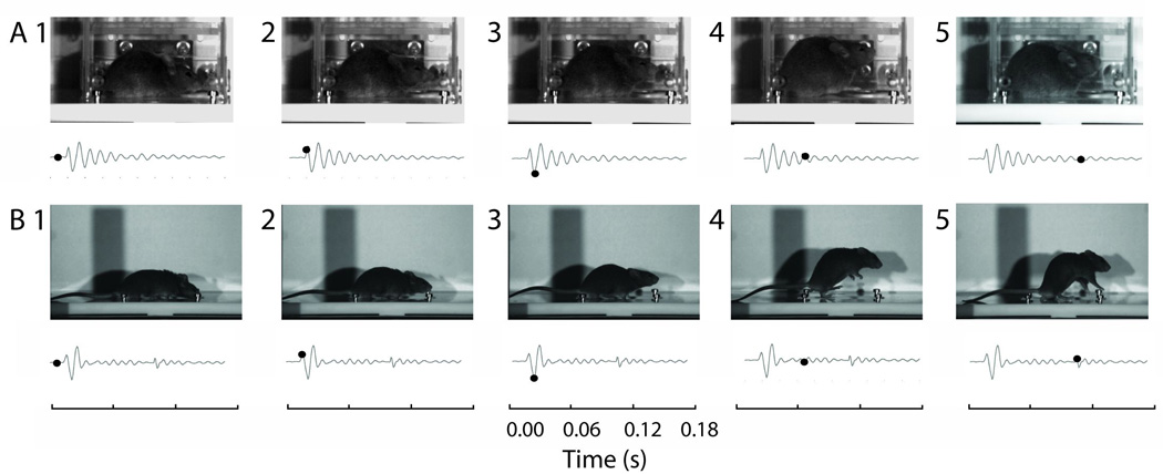
Different phases of mouse movement during a startle response recorded by a high-speed video camera. (A) The major phases of startle movements recorded inside a Plexiglas restrainer. The startle response waveform was recorded simultaneously with the video recording using a piezoelectric sensor (piezoelectric startle plate waveforms are shown below every picture frame). The black dot on the startle waveform indicates the time when the corresponding pictures were taken. (B) Mouse movement during a startle response without restrainer. Also see supplemental materials for video recordings.
Two separate video recording sessions were performed. In the first session, the mouse was restrained in a small cage placed on top of the startle plate. In the second session, the mouse was placed on the startle plate without a restrainer. The restrained paradigm allowed for evaluation of the startle waveform produced in conditions close to those of typical experimental conditions. During typical experimental conditions mice are restrained in an acoustically transparent restrainer (Longenecker and Galazyuk 2012). The unrestrained paradigm permitted the mouse to use its full range of motion during an ASR.
2) Developing a mathematical, automated, startle waveform classifier
Video analysis revealed that an ASR in mouse produced a stereotyped waveform from the piezoelectric startle plate (Fig. 2). Further analysis revealed that the first three peaks of this waveform, the first positive (P1), the first negative (N1), and the second positive (P2) peak, are necessary to identify it from non-startle waveforms. An automated classifier was developed to identify this stereotyped waveform and separate startle data from noise. Three criteria are used by the classification. First, the waveform must contain the three peaks of interest, second, these peaks have the appropriate timing, and third, each peak’s magnitude is greater than the trial specific threshold.
Figure 2.

Automated startle waveform identification. The following startle waveform parameters were required for identification of a waveform as a startle. The first and second positive peaks (P1 and P2) as well as the first negative peak (N1) occur within previously identified time windows (indicated by black horizontal bars) and the absolute amplitude values of the peaks exceed the trial-specific positive and negative thresholds. The grey vertical bar indicates the startle stimulus.
The timing of the peaks of interest was automatically identified using an iterative procedure implemented in a custom MATLAB script. This established timing windows for our automated ASR classifier. An initial dataset (Dataset 1) was collected using 400 randomly chosen startle trials using stimulus intensities ranging from 60 to 120 dB SPL from eight male CBA/CaJ mice (4–9 months of age). The timing windows were calculated in two steps. First, large timing windows (TP1, TN1 and TP2) were computed for each peak (P1, N1 and P2) by plotting the mean waveform of all 400 trials. TP1, TN1 and TP2 were taken as the time points where the average waveform crossed zero (Fig. 3). Because of the reliable latency of this reflexive movement, any waveform from a true startle event will have its P1, N1 and P2 peaks within these time windows. These initial large time windows were used as a starting point to refine the windows used in the automated ASR classifier. As overly large time windows would increase the probability of non-startles and/or random animal movement being misclassified at startles, a second dataset of 200 trials (dataset 2) was collected to calculate more precise timing windows for each peak of interest. Prior experiments have demonstrated that startle stimuli of 110dB SPL elicit a reliable startle response (Longenecker & Galazyuk 2012). Therefore, dataset 2 trials used a startle stimulus intensity of 110dB SPL. These data were collected from the same 8 male CBA/CaJ mice (4–9 months of age) used in dataset 1. The time points of the maxima of the positive peaks (P1 and P2) and the minimum of the negative peak (N1) were extracted for each trial. The mean ± 2 standard deviations, for each peak, across all trials were then used to define the refined timing windows (P1win, N1win and P2win, Fig. 4).
Figure 3.

Obtaining overly large time windows (TP1, TN1 and TP2) for peaks in a startle waveform. TP1, TN1 and TP2 are derived from the time points at which the mean waveform of 400 randomly selected trials crosses zero (indicated by ‘x’s).
Figure 4.

Method for determination of the time windows for P1, N1 and P2 peaks on a startle waveform for automated startle identification. Precise timing of each peak is extracted, using the overly large time windows previously calculated. 100 example waveforms are shown, superimposed. Startle stimulus was 110dB SPL for each trial. The timing of the P1, N1 and P2 peaks in every startle waveform are indicated by blue, red, and green dots, respectively. The grey vertical bar indicates the startle stimulus. Black horizontal bars indicate the time windows calculated for each peak (P1, N1 and P2) using the timing of the apex of the peak in each trial (mean time from all trials ± 2 SD).
Once the automated classifier has identified the three peaks of interest and confirmed each peak occurs within its previously calculated time window (P1win, N1wind and P2win), it then checks each peak breaks threshold. Values are computed for both positive and negative thresholds (pT and nT) on a trial-by-trial basis. Positive thresholds were defined as the mean of all positive values in the waveform preceding the startle stimulus, plus 2 standard deviations. The negative threshold was defined as the mean of all negative values preceding the startle stimulus minus 2 standard deviations (Fig. 2). For each trial, positive peaks (P1 and P2) were defined as the maximum value within P1win or P2win with 3 ms of smaller values both before and after. Negative peaks (N1) were defined as the minimum value within N1win with 3 ms of larger values both before and after.
The following criterion was used to automatically determine if an ASR occurred: all three peaks occurred in the time windows specified and (P1>pT) & (N1<nT) & (P2>pT).
3) Testing the accuracy of the automated classifier
To assess the accuracy of the automated classifier, a third dataset (dataset 3) at startle stimulus intensities of 70, 85, 100 and 115 dB SPL was collected from eight novel male CBA/caJ mice (4–9 months of age). 100 trials were collected at each intensity for a total of 400 trials. Markers indicating the stimulus intensity were removed and the order of the trials was randomized. This step ensured researchers assigning trials as startle or no-startle by visual analysis (manual classification) had no idea of the specifics of the individual trials. The randomized dataset was then analyzed by both the automated classifier and manual classification. The dataset was then reordered to allow analysis of the accuracy of the automated classification compared with the manual classification, across stimulus intensities. The accuracy of the automated classifier was assessed using a two-way ANOVA.
4) Comparisons with other methods
A final dataset (dataset 4) was used to compare the accuracy of the automated startle classifier with other commonly used ‘separation’ methods. 100 trials at intensities of 0, 80 and 110dB SPL were collected from a novel group of eight male CBA/caJ mice (4–9 months of age), making a dataset of 300 trials in total. Four separation methods where then used to separate these trials into startle and non-startle groups. The separation methods tested where:
Method 1 (Auto) the automated classifier outlined in this manuscript.
Method 2 (Threshold) separates trials based on calculating a threshold from the pre-stimulus data. The largest value found in the force plate waveform before the startle stimulus is used to set this threshold. If the largest value after the startle stimulus is greater than this, it is deemed a startle.
Method 3 (RMS) calculates the root mean square (RMS) of the values for the 100ms preceding the stimulus and the 100ms immediately after the stimulus. If the post-stimulus RMS value exceeds that of the pre-stimulus RMS, the trial is classified as a startle.
Method 4 (Max) does not separate trials but includes all trials as startle data, taking the largest positive value in the waveform after the stimulus was played as the amplitude of the startle. While this approach does not distinguish between startle and non-startle trials, it was included in our analysis since it is the method used in some commercially available startle equipment.
The accuracy of these methods was then computed as percentage agreement with manual classification. Trials in which the separation method and the manual classification both identified a startle were deemed ‘Correct startle’ trials, where both agreed there was no startle were deemed ‘Correct no-startle’ trials. Trials deemed as ‘Misclassified as startle’ were those in which the separation method classified a trial as containing a startle, where the manual classification did not. Trials termed ‘Misclassified as no-startle’ where those in which the separation method classified the trial as not containing a startle, while the manual classification deemed that it did.
The percentage of trials falling into the four possible outcomes; ‘Correct startle’, ‘Misclassified as startle’ (Fig. 8A) ‘Correct no-startle’ and ‘Misclassified as no-startle’(Fig. 8B) where calculated. These values were calculated as (‘number of trials in category for separation method’/’number of trial in category for manual classification’) × 100. For example, the percentage of trials classified as ‘Correct startle’ was the number of ‘Correct startle’ trials divided by the total number of startle trials classified as such by manual classification. This enables observations regarding the specific accuracies or inaccuracies of each separation method.
Figure 8.

Comparison of the effectiveness of four different startle identification methods (‘Auto’, ‘Thresh’, ‘RMS’ and ‘Max’) at different startle stimulus intensities (0, 80 and 110 dB SPL). All four methods were compared to manual classification to calculate values for percentage classified and percentage misclassified. (A) Percentage classified as ‘Correct nostartle’ and ‘Misclassification as startle’. (B) Percentage classified as ‘Correct startle’ and ‘Misclassification as no-startle’. (C) Agreement with Manual Classification for the four methods across startle level, calculated as (% ‘Correct startle’ + % ‘Correct no-startle’) / 2.
To enable a quicker assessment of any separation method, a value of ‘agreement with manual classification’ (Fig. 8C) is calculated. ‘Agreement with manual classification’ is derived by summing the values for percentage correctly classified as ‘Correct startle’ and ‘Correct no startle’, and then divided by 2. As such, any separation method that classifies all trials as startles will get a value of 100% for ‘Correct startle’ and a value of 0% for ‘Correct no-startle’. Therefore a value of 50% for ‘agreement with manual classification’ will be considered chance.
4) Normalizing for animal mass in startle data
A major issue with interpreting startle data is the ability to compare outputs from animals of different masses. For a given movement amplitude (i.e., displacement), an animal with a greater mass will exhibit a larger force. Hence, the amplitude of the startle, as measured by the startle plate, will be greater for large animals than for small animals, even when both animal’s startle responses are the same. To be able to compare startle behavior of animals of different mass, or the same animal over a long time period (where the mass may change), it is important to be able to normalize the response magnitude to the mass of the animal. To do this, we adopted a set of simple mathematical extrapolations to convert force into center-of-mass displacement (COMd). COMd equates to the change in vertical position of the animal’s center-of-mass. We used standard principles of force plate ergometry (e.g., Manter 1938, Cavagna & Kaneko 1977) to calculate the finite change in COM height that result from the accelerations of the animal’s startle movement. First, from Newton’s second law of motion (F=ma), acceleration can be calculated by dividing the startle plate force data by the animal’s body mass. Then, changes in COM height can be calculated as the cumulative double integral of acceleration with respect to time (Young 2009). Constants for these integrations were set to zero, on the assumption that there was, on average, no net upward movement of the COM prior to the initiation of the startle response. Matching positional changes to the raw waveforms provides an intuitive graphical means of interpreting the ultimate biomechanical meaning of the startle waveform. Additionally, as we argue below, the maximum displacement of the animal’s COM during the startle response provides an accurate metric of overall startle magnitude. It is important to note that the animals mass must be measured prior to each recording to allow precise measurements of COMd. In this study, researchers carefully measured the mass of each animal by weighing them on a calibrated Ohaus Scout Pro digital scale, immediately prior to inserting the animal into the startle chamber.
Results
1) Correlating animal movements with components of the startle plate waveform
To enable reliable identification of startle data from noise, we time-coupled video recordings made during a startle event with changes in the waveform generated by the piezoelectric startle plate. Each waveform produced by the startle plate during these video recordings was then superimposed onto the corresponding video (Fig. 1, Supplemental Video 1).
Startle on piezoelectric plate with restrainer
Startle data in mouse is typically collected while the mouse is loosely restrained, allowing enough movement for a startle, while retaining the animal over the startle plate. The first experimental condition tested with high-speed video replicates this level of restraint. This condition revealed that a startle movement results in a stereotyped waveform from the piezoelectric startle plate (Fig. 1). Video analysis revealed the first positive peak (P1) of the startle waveform corresponds to a downward force of the animal just prior to any vertical movement (Fig. 1a and Fig. 1b, panel 2). The first negative peak (N1) corresponds to the maximum vertical displacement of the COM (Fig. 1a and Fig. 1b, panel 3). Due to the confined nature of the restrainer, we could not link the remaining phases of the waveform with the animal’s movement. Therefore, we conducted similar recording sessions using the same startle plate without a restrainer.
Startle on piezoelectric plate without restrainer
To further explore the mechanics of the startle in mouse, animals were placed on the same startle plate without any restraint. The lack of restraint allowed us to record the full range of movement and directly link these movements to the separate phases of the startle waveform previously identified (P1, N1 and P2).
Figure 1b shows a sequence of still frames demonstrating five phases of the animal’s movements during a startle. We can loosely think of these as ‘1 - resting’, ‘2 - pushing off’, ‘3 - lifting off’, ‘4 - airborne’ and ‘5 - landing’ (Fig. 1b panels 1–5, respectively). We have linked two of the three peaks of interest with a specific and well defined phase of the animal’s movement during a startle. P1 corresponds to a net downward force prior to upward movement, or ‘pushing off’, and N1 corresponds to the animal unweighting from the startle plate (initiating a movement large enough to completely loose contact with the plate in some cases), or ‘lifting off’. We have no defined movement associated with P2, however.
2) Automated classifier
Time windows for the three peaks used by the automated startle classifier
The time windows used by the automated classifier were calculated using two steps. First large time windows were extracted from the zero crossing points of a mean waveform of 400 randomly-picked waveforms. These were used as starting points for more refined calculations, with final windows resulting from the mean ± 2 standard deviation of the timing of the peaks from 200 trials at 110 dB SPL stimulus intensity (see methods and Fig. 4).
This process resulted in time windows of 17.30 to 22.32ms, 30.37 to 38.39ms and 44.52 to 57.31ms for peaks P1, N1 and P2 respectively (Table 1 and Fig. 3).
Table 1.
Timing of the 3 peaks from startle waveforms used for automated startle classification. Values derived from 200 trials, each using a startle stimulus of 110dB SPL (dataset 2). All units are in milliseconds.
| P1 | N1 | P2 | |
|---|---|---|---|
| Mean | 19.81 | 34.38 | 50.91 |
| Standard deviation | 1.25 | 2.00 | 3.20 |
| Timing window (mean ± 2 SD) | 17.30–22.32 | 30.37–38.39 | 44.52–57.31 |
Automatic classification of waveforms
Waveforms were separated as startles or non-startles by the automatic classifier as described in the methods. The dataset used (dataset 3) consisted of a total of 400 startle responses, recorded from eight six-month old CBA/CaJ mice. These 400 waveforms can be divided into four groups each containing 100 trials at four different startle stimulus intensities (70, 85, 100 and 115 dB SPL). Out of the 400 waveforms comprising dataset 3, 213 were classified as startles based on criteria outlined in the methods, while the remaining 187 were classified as no-startle.
Manual classification of startle waveforms
The dataset analyzed by the automatic classifier (dataset 3) was also used to separate startle trials by manual classification as described in the methods. Manual classification identified 235 of the 400 waveforms as startles and the remaining 165 as no-startle. Inter experimenter consistency was assessed using both Fleiss’ kappa and Krippendorff’s alpha. Values were 0.865 for both metrics, indicating very good levels of agreement between the three researchers used. Manual classification is therefore consistent, making it a reliable baseline for comparison with other automated methods. The mean of all the waveforms from dataset 3 grouped as no-startle and startle, for both manual and automated classification, are shown in Figure 5. These traces are grouped by startle stimulus intensity.
Figure 5.


Manual and automatic startle waveform classification. Top panels show manual classification; bottom panels show automatic classification. 100 waveforms where analyzed for each stimulus intensity (115, 100, 85 and 70 dB SPL). The number of trials classified as startle and no-startle are indicated in the top left of each panel, as such, each row totals 100 trials. (A–D) Mean waveform of all trials classified as startle. (E–H) Mean waveform of all trials classified as no-startle. Error bars are standard deviation. Startle stimulus is represented by a vertical grey bar. All axis are on the same scale.
Effectiveness of automatic startle identification compared to manual
Manual and automatic startle identification generated very similar groups (Fig. 4). Very few waveforms manually classified as no-startles were classified as startles by the automated categorization (1.2%, 2/165). Similarly, few waveforms manually classified as startles were classified as no-startles by automated analysis (10.2%, 24/235). A two-way ANOVA revealed that there was no significant effect of classification method on the magnitude of the 3 peaks (P1: p=0.526, N1: p=0.488, P2: p=0.529). A significant main effect was found of signal intensity on the magnitude of all 3 peaks (P1, N1 and P2: p<0.001), where more intense sounds were likely to elicit a higher magnitude ASR. There was no interaction between intensity and classification method (P1: p=0.956, N1: p=0.955, P2: p=0.967), indicating that the manual and automatic classifiers were equally good at detecting ASRs across intensities (see Fig. 7).
Figure 7.

Mean magnitude of each peak of interest (P1, N1 and P2) as classified by manual classification (white bars) and the automated classifier (grey bars). A two-way ANOVA revealed that there was no significant effect of classification method on the magnitude of the 3 peaks (P1: p=0.526, N1: p=0.488, P2: p=0.529) and no interaction between intensity and classification method (P1: p=0.956, N1: p=0.955, P2: p=0.967), indicating that the manual and automatic classifiers were equally good at detecting ASRs across intensities. Error bars are standard deviation.
3) Assessing different classification methods
To test the accuracy of the automated classification against other separation methods, a novel dataset (dataset 4) of 300 different startle trials from a novel group of eight 4–9 month old male CBA/CaJ mice was analyzed. 100 trials at three different intensities (0, 80 and 110dB SPL) were collected. These 300 waveforms were manually classified and the results were compared to those from four different startle separation methods. It is assumed that the manual classification, carried out by three experienced researchers, yields the correct answer.
The four startle separation methods tested were:
Method 1: Automated startle classifier.
Method 2: Threshold the data based on the pre-stimulus movement.
Method 3: Compare root mean square (RMS) values of the pre-stimulus and the post stimulus waveform.
Method 4: Use absolute maximum value after stimulus onset (not truly a separation method, but included here as it is often the method used in commercially available startle software).
Pooling across all three stimulus intensities, the automated classification method showed the closest agreement with manual classification (Correctly classified trials = 296/300, Cohen’s κ = 0.973, p < 0.001) than either the threshold method or the RMS method (threshold: Correctly classified trials = 229/300, Cohen’s κ = 0.522, p < 0.001; RMS: Correctly classified trials = 201/300, Cohen’s κ = 0.331, p < 0.001). As expected, the max method performed close to chance (Correctly classified trails = 153/300, Cohen’s κ = 0, p = 1), identifying all 147 no-startle waveforms (49% of total) as startles.
Separating trials by stimulus intensity revealed that manual identification by experienced researchers indicated that none of the 0dB waveforms were startles. Whereas the automated method presented here accurately classified all of these 100 waveforms as no-startles, the threshold method and the RMS method inaccurately classified 34% and 60% as startles, respectively. The max method, by definition, inaccurately classified 100% as startles.
Manual identification identified 47 of the 80 dB waveforms as no-startles and 53 as startles. Of the four separation methods, our automated method showed the best agreement with manual classification (46 no-startle/54 startle, Cohen’s κ = 0.94, p < 0.001). Both the threshold and RMS methods performed worse than the automated method, overestimating the number of startle events (threshold: 10 no-startle/90 startle, Cohen’s κ = 0.223, p < 0.001; RMS: 8 startle/92 no-startle, Cohen’s κ = 0.179, p = 0.002). The max method, again by definition, incorrectly identified 100% of the no-startle waveforms as startles (Cohen’s κ = 0, p = 1).
Finally, manual classification identified all of 110 dB waveforms as startles. The automated method correctly identified 99% of these waveforms as startles, whereas the other three methods correctly identified all of the waveforms as startles.
To further investigate how each classification method compared with manual classification, the percentage of trials correctly classified (‘Correct startle’ and ‘Correct no startle), as well as the percentage misclassified (‘Misclassified as startle’ and ‘Misclassified as no-startle) are shown in table. 2. Values for ‘agreement with manual classification’ were also calculated as ‘Correct startle’ + ‘Correct no-startle’/2 (see Table. 2 and Fig. 8).
Table 2.
Percentage agreement between four possible startle separation methods and manual classification of startle waveforms. ‘Auto’: the automated classifier, ‘Thresh’: uses just a pre-stimulus threshold, ‘RMS’: includes trials with a higher RMS post stimulus compared to pre-stimulus, ‘Max’: includes all trials, reporting the maximum post-stimulus value. ‘Correct startle’: the separation method correctly identifies a startle. ‘Misclassified as no-startle’: the separation method incorrectly classifies a startle as a no-startle. ‘Correct no-startle’: the separation method correctly identifies a no-startle. ‘Misclassified as startle’: the separation method incorrectly identifies a no-startle as a startle. Agreement with Manual Classification for the four methods across startle level, calculated as (% ‘Correct startle + % ‘Correct no-startle) / 2).
| ‘Correct Startle’ |
‘Misclassified as no-startle’ |
‘Correct no-startle’ |
‘Misclassified as startle’ |
Agreement with manual classification |
||
|---|---|---|---|---|---|---|
| 0dB | Auto | N/A | N/A | 100 | 0 | 100 |
| Thresh | N/A | N/A | 66 | 34 | 66 | |
| RMS | N/A | N/A | 40 | 60 | 40 | |
| Max | N/A | N/A | 0 | 100 | 0 | |
| 80dB | Auto | 98.1 | 1.9 | 95.7 | 4.3 | 96.9 |
| Thresh | 100 | 0 | 21.3 | 78.7 | 60.6 | |
| RMS | 100 | 0 | 17 | 83 | 58.5 | |
| Max | 100 | 0 | 0 | 100 | 50 | |
| 110dB | Auto | 99 | 1 | N/A | N/A | 99 |
| Thresh | 100 | 0 | N/A | N/A | 100 | |
| RMS | 100 | 0 | N/A | N/A | 100 | |
| Max | 100 | 0 | N/A | N/A | 100 |
All separation methods were successful at correctly identifying startle trials. Percentages correct for ‘Correct startle’ were between 98 and 100% for all methods at all stimulus intensities tested which contained startles (Table 2, Fig8A). Across all intensities, the automated method (‘Auto’ in Fig. 8 and Table 2) far outperformed all other methods at identifying no-startles, shown by a higher ‘Correct no-startle’ percentage (95.7–100% compared to 0–66%).
The automated method closely followed the classification given by manual classification, outperforming other methods at lower stimulus intensities (0dB =100%, 80dB =96.9%, see Table. 2 and Fig. 8C). All separation methods worked well at 110dB, achieving values of 99–100% for ‘agreement with manual classification’.
There were no values for ‘Correct startle’ and ‘Misclassified as no-startle’ for the 0dB SPL stimulus trials as there were no startles elicited at this intensity. Similarly there are no values for ‘Correct no-startle’ and ‘Misclassification as startle’ for the 110dB SPL trials as all trials resulted in a startle. This is represented by N/A in Table 2 and Figure 8.
4) Use of center of mass displacement to quantify startle magnitude and normalize for animal mass
Calculating center of mass displacement (COMd) is possible from startle data. COMd is a measure of the vertical displacement of the center of mass. It is useful when reporting startle data as it incorporates the animals mass, accounting for this variable (see methods).
Figure 10 shows the results of using COMd compared to raw force data. As the mass of the animal increases, it corresponding COMd will decrease, for a given force (Fig. 10). Figure 10A illustrates this using an actual startle plate waveform (black trace) and 5 arbitrarily chosen animal masses. As the animals mass decreases, the COMd achieved increases for the same raw force plate waveform. Figure 10B and C represent the same relationship in a different way. In both panels actual startle plate waveforms are presented from 2 different mice. The amplitude of these force data are nearly identical (0.435N and 0.437N for panel B and C respectively). However, animal #14 (Fig. 10B) had a mass of 26.1g, while animal #19 (Fig. 10C) had a mass of 43.2g. Due to the relationship between force and mass, animal #14 therefore had to have a greater startle response than animal #19. This is shown clearly by the COMd traces (red lines), after the mass of the animals is considered, the startle response by animal #14 was far larger than that of animal #19 (COMd of 1.192mm and 0.649mm, respectively).
Figure 10.
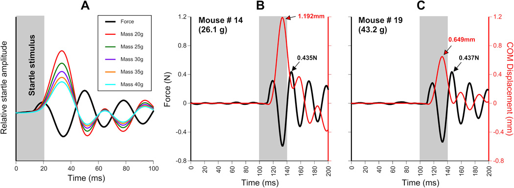
Effect of animal mass on COM displacement (position). (A) Black trace = force output of piezoelectric startle plate. Color traces = corresponding COM positions for an animal of that mass. Note that a 20g animal achieves twice the COMd (‘height jumped’) of a 40g animal, while exerting the same force on the startle plate. (B) Force plate waveform (black trace) for a 26.1g animal and its corresponding COMd position (red trace). (C) Force plate waveform (black trace) for a 43.2g animal and its corresponding COMd position (red trace). Note the maximum force for both animals is very similar (0.435N and 0.437N) whereas the COMd differs greatly (1.192mm and 0.649mm) due to the difference in mass between the two animals (26.1g and 43.2g). Absolute force may not be the best metric for startle amplitude.
Moreover, as a metric of startle magnitude, absolute COM displacements correlate to stimulus intensity as well as the peak amplitude of the startle waveform. Non-parametric Spearman’s rank-based correlations of startle magnitudes against a 60–120 dB SPL range of startle stimuli demonstrate that there is a similar level of association between stimulus intensity and COMd (rho=0.629, p<0.001) as between stimulus intensity and maximum waveform amplitude (rho=0.596, p<0.001). Thus, these two measures of startle magnitude correlate equally well with stimulus intensity.
Discussion
Startle identification
There is currently no consensus on how to assess the occurrence of a startle. This is a critical problem, as the probability of a startle occurring in any given trial varies greatly depending on the experimental paradigm. Furthermore, at low stimulus intensities, a significant number of successful startles have small magnitudes (Fig. 5D), but should be included in any analyses. If an animal’s movement before the stimulus has a higher or even similar amplitude to a small startle, these data are often discarded. Here we demonstrated an improved approach for identifying the startle-related waveforms produced on piezoelectric startle plates that is virtually independent of startle magnitude. We utilized high-speed video to correlate the movements of the animal with components of the startle waveform. We demonstrated how to interpret the waveform and offered evidence as to which specific component of the waveform correlates with specific phases of the startle movement. We then developed a robust approach to automatically distinguish true startle events from noise with ~88% accuracy, even at very low startle amplitudes. We also introduce a new metric, COMd, which not only gives a salient unit with which to report startle magnitude, but also normalizes force plate data for the mass of the animal.
1) Correlating animal movements with components of the startle plate waveform
Initial high-speed video experiments revealed a stereotyped waveform produced during a startle event. We were successful at correlating the first 2 peaks of interest in this waveform, P1 and N1, with distinct phases of the animal’s movement. P1 corresponds to a ‘pushing’ on the plate in preparation for the upward movement of the startle (Fig. 1 Panel 2). N1 corresponds to the initial ‘unweighting’ of the plate, starting the animal’s upward trajectory (Fig. 1 panel 3). We could not correlate the third peak, P2, with a clear and distinct movement. It is possible that this peak is due to an oscillation of the Plexiglas startle plate, as a result of the initial weighting and unweighting of the plate during the P1 and N1 phase. Experiments to assess the resonance of the plates indicated that these plates will ‘ring’ for an extended period of time as a result of a single movement.
2) Automated classifier
The stereotyped waveform associated with a startle allowed for visual classification of waveforms by experienced researchers, a process we termed ‘manual classification’. Throughout this study we have used manual classification as the basis to assess varies mathematical methods to separate startle trials. The manual classification of startle data consisted of three experienced researchers deciding, by eye, whether each trial consisted of a startle or not. This is the best method we currently have to validate other methods. Manual classification has proven to be consistent, with little inter-experimenter disagreement, as shown by high values of Fleiss’s kappa and Krippendorff’s alpha (0.865 in each case). However, it is unlikely to be perfect as some inherent human error is likely. It is quite possible that some trials that were manually classified as startle are not (for example figure 6D). Similarly some trials classified as no-startle by the manual method may be true startles (figure 6A). We see this as further reason to develop an automated method based on a repeatable mathematical structure, rather than relying upon subjective opinions of human researchers.
Figure 6.

Examples of startle waveforms that were misclassified by manual or automatic classification. Black traces indicated misclassified waveforms. Grey traces are a typical startle waveform for comparison (the same on all panels).
The need to be able to separate startle data in an automated way, based upon mathematical criteria lead to the development of our automated classifier. An important aspect of this classifier was the ability to separate startle trials, regardless of the startle amplitude. The automated classifier has very good agreement with manual classification across stimulus intensities and startle amplitudes (Fig. 5). Results from a two-way ANOVA on the amplitudes of each of the three peaks of interest show no significant difference between those classified by manual classification and the automated classifier (P1: p=0.526, N1: p=0.488, P2: p=0.529), regardless of stimulus intensity (Fig. 7).
3) Assessing different classification methods
The lack of standardized methods for handling startle data make it impossible to directly compare the automated method with every startle separation method used. Here we compare the automated classifier to three methods that are commonly used on startle data: 1) setting a pre stimulus threshold that needs to be crossed, 2) calculating the RMS of the pre and post-stimulus waveform and 3) simply using the largest positive value post-stimulus without any separation of trial (for more details see methods section 4). We show that for high startle stimulus intensities many separation methods are successful (Table. 2). Such stimulus intensities often result in a high probability of a startle occurring and a large amplitude startle (Fig. 5). As such, it is often at lower stimulus intensities where a robust separation method is most useful. We demonstrate that at lower intensities our automated classifier outperforms all others (Table. 2, 80dB), especially at correctly rejecting no-startles (Fig. 8B), effectively eliminating noise from the data to be analyzed.
4) Use of center of mass displacement to quantify startle magnitude and normalize for animal mass
There is currently no consensus of how to report a startle magnitude. Some researchers will report force (N) without considering the effect of the animal’s mass, yet others will report the voltage (mV) value generated by the sensor in the startle plate. We advocate the simple conversion of force to COM displacement when reporting startle amplitudes. The mathematical procedures outlined above (cumulative double integration of the raw waveform) provide a means by which researchers can normalize their data for the mass of individual animals, eliminating this otherwise confounding variable. It is our firm belief that this benefit alone makes these conversions a valuable tool to anyone utilizing startle reflexes in their work. This is especially true of studies requiring animals to be tested over long periods of time where the mass of each animal is likely to change. We also demonstrate that COMd is as faithful a measure of startle magnitude as absolute magnitude of the largest peak. We thus advocate use of this technique whenever the quantification of startle magnitude is of interest.
Replication of our automated classifier
Due to the wide variety of equipment and data formats used to collect startle data, it is beyond the scope of this work to supply ‘plug-and-play’ code for our automated classifier. We do, however, strongly encourage its adoption by researchers interested in quickly and easily separating startle data from that of noise. As such, we offer the following steps as a guide for researchers wishing to replicate our method on their own data.
Step 1. Confirm that the test apparatus utilizes a piezoelectric sensor; this method is optimized for sensors of this type.
Step 2. Identify whether your system outputs a stereotyped waveform similar to that in Figure 2. To do this, calculate and view the average response from 100 trials that are likely to elicit a startle response in your model (e.g. trials with a high stimulus intensity).
Step 3. Create conservatively large peak timing windows based on the mean waveform of 400 randomly chosen startle trials. Use the zero crossing points of the peaks (see Fig. 3).
Step 4. Using your conservatively large windows, for each of the 400 trials find the value for each peak (largest positive value for P1 and P2, largest negative for N1) and its corresponding time point in milliseconds. Before using these values in step 5, ensure that the values taken are the very tip of the peak.
Step 5. Calculate the mean times of all the peaks (P1, N1 and P2) identified in step 4. The mean time minus 2 standard deviations will be the start point of the refined window for that peak. The mean time plus 2 standard deviations will be the end point.
- Step 6. Create the automated classifier. The automated classifier needs to do three things;
- For each trial, calculate the positive threshold (pT) and the negative threshold (nT). pT is the mean of all positive values preceding the startle stimulus, plus 2 standard deviations. nT is similarly the mean of all negative values preceding the startle stimulus minus 2 standard deviations. Note that these thresholds are created on a trial-by-trial basis
- Identify peaks within the refined time windows calculated in step 5. Ensure that they are actual peaks, surrounded to either side by decreasing values (or by increasing values for N1)
- The trial is deemed a startle if P1, N1 and P2 occur within the time windows specified and if P1 and P2 are above pT, while N1 is below nT.
Step 7. Assess the accuracy of the automated classifier. The two methods outlined in this manuscript both rely on first manually assigning a dataset of trials as startle or no-startle. Once this is done, the accuracy of the automated classifier can be assessed by calculating percentage correct values and/or investigating the difference between the values found for the peaks designated as startle by manual classification and those designated as startle by the automated classifier.
Conclusions
Here we offer a method to confidently remove a high percentage of noise from startle data. Our method is unique in that we go to great lengths to demonstrate that the startle movement in the mouse results in a stereotyped and recognizable waveform from the piezoelectric sensor. We show that this stereotyped waveform can be successfully identified and used to visually separate trials by experienced researchers, a process we term ‘manual classification’. We further show that this waveform can be mathematically and automatically separated from waveforms that do not conform and are thus noise. We demonstrate that this automated classifier has a high correlation with manual classification of startle trials, even at low startle amplitudes. Comparisons with other startle separation methods reveals many are successful at very high startle amplitudes but only the automated classifier described here is successful at lower startle amplitudes. We then demonstrate a method to convert force data into COMd. COMd conversion allows an intuitive unit for startle amplitude (mm) as well as eliminating a massive confound in startle data, that of the animals mass.
Though our method was developed in mouse, we believe it should be easily adapted to other laboratory animals. Researchers who currently add behavioral trials to reduce the effect of noise in their data would likely reduce the total time they need to conduct experiments if our approach were adopted. To adapt our approach to laboratory animals other than mice it would be necessary to analyze the shape of the startle waveform and the timing of its individual components. Assuming the shape is the same, which is likely if a piezoelectric sensor/Plexiglas platform is utilized, laboratories with access to simple programming capabilities (MATLAB, Visual Basic, Python, etc.) can then write their own custom, automated classifier program to automatically separate out startle data from noise.
Supplementary Material
Figure 9.

Mathematical conversion of startle force to center of mass (COM) displacement. (A) Force output of startle plate. (B) Force in A converted to acceleration (F=ma). (C) Velocity, calculated from acceleration. (D) Position of animal’s COM, or ‘height jumped,’ calculated from velocity. The initial extrapolation, from force to acceleration, requires knowledge of the animal’s mass (F=ma) and incorporates this mass into the equation. As such, animal mass is normalized when converting force data into COMd.
Highlights.
We explored the fundamental movement of the ASR in mouse, utilizing high-speed video to record startle movements.
We created an automated program that classifies raw force traces into startles and non-startles
The accuracy of this new approach was then compared with other common methods for startle data analysis.
We suggest a method for normalizing for animal mass by combining raw force data with each individual animal’s mass into a simple mathematical equation.
Acknowledgments
We would like to acknowledge Olga Galazyuk for converting the automated classifier into a fully functional automated program. We would also like to thank Dr. Sharad Shanbhag, Dr. Chris Vinyard and Greg Nelson for their comments on earlier versions of this manuscript. This research was supported by grant R01 DC011330 to A.V. Galazyuk, R01 DC013314 to M.J. Rosen, R01 DC000937-23 to J.J. Wenstrup and 1F31 DC013498-01A1 to R. J. Longenecker from the National Institute on Deafness and Other Communication Disorders of the U.S. Public Health Service, and grant IOS-1146916 to Jesse W. Young from the National Science Foundation.
Abbreviations
- ASR
Acoustic Startle Reflex
- P1(t)(win)
First positive peak of the startle waveform (timing)(window)
- P2(t)(win)
Second positive peak of the startle waveform (timing)(window)
- N1(t)(win)
First negative peak of the startle waveform (timing)(window)
- LED
Light emitting Diode
- pT
postitive threshold
- nT
negative threshold
- COMd
Center of mass displacement
- dB SPL
decibels sound pressure level
Footnotes
Publisher's Disclaimer: This is a PDF file of an unedited manuscript that has been accepted for publication. As a service to our customers we are providing this early version of the manuscript. The manuscript will undergo copyediting, typesetting, and review of the resulting proof before it is published in its final citable form. Please note that during the production process errors may be discovered which could affect the content, and all legal disclaimers that apply to the journal pertain.
References
- Acocella CM, Blumenthal TD. Directed attention influences the modification of startle reflex probability. Psychological Reports. 1990;66:275–285. doi: 10.2466/pr0.1990.66.1.275. [DOI] [PubMed] [Google Scholar]
- Allen PD, Schmuck N, Ison JR, Walton JP. Kv1.1 channel subunits are not necessary for high temporal acuity in behavioral and electrophysiological gap detection. Hearing Research. 2008;246:52–58. doi: 10.1016/j.heares.2008.09.009. [DOI] [PMC free article] [PubMed] [Google Scholar]
- Buckland G, Buckland J, Jamieson C, Ison JR. Inhibition of startle response to acoustic stimulation produced by visual prestimulation. Journal of Comparative and Physiological Psychology. 1969;67(4):493–496. doi: 10.1037/h0027307. [DOI] [PubMed] [Google Scholar]
- Carlson S, Willott JF. The behavioral salience of tones as indicated by prepulse inhibition of the startle response: relationship to hearing loss and central neural plasticity in C57BL/6J mice. Hearing Research. 1996;99:168–175. doi: 10.1016/s0378-5955(96)00098-6. [DOI] [PubMed] [Google Scholar]
- Cavagna GA, Kaneko M. Mechanical work and efficiency in level walking and running. J. Physiol. 1977;268:467–481. doi: 10.1113/jphysiol.1977.sp011866. [DOI] [PMC free article] [PubMed] [Google Scholar]
- Davis M, Gendelman DS, Tischler MD, Gendelman PM. A primary acoustic startle circuit: Lesion and stimulation studies. The Journal of Neuroscience. 1982;2(6):791–805. doi: 10.1523/JNEUROSCI.02-06-00791.1982. [DOI] [PMC free article] [PubMed] [Google Scholar]
- Davis M, Menkes DB. Tricyclic antidepressants vary in decreasing α2-adrenocepter sensitivity with chronic treatment: Assessment with clonidine inhibition of acoustic startle. Br. J. Pharmac. 1982;77:217–222. doi: 10.1111/j.1476-5381.1982.tb09288.x. [DOI] [PMC free article] [PubMed] [Google Scholar]
- Franklin JC, Moretti NA, Blumenthal TD. Impact of stimulus signal-to-noise ratio on prepulse inhibition of acoustic startle. Psychophysiology. 2007;44:339–342. doi: 10.1111/j.1469-8986.2007.00498.x. [DOI] [PubMed] [Google Scholar]
- Gerrard RL, Ison JR. Spectral Frequency and the Modulation of the Acoustic Startle Reflex by Background Noise. Journal of Experimental Psychology: Animal Behavior Processes. 1990;16(1):106–112. [PubMed] [Google Scholar]
- Graham FK. The more or less startling effects of weak prestimulation. Psychophysiology. 1975;12:238–248. doi: 10.1111/j.1469-8986.1975.tb01284.x. [DOI] [PubMed] [Google Scholar]
- Grillon C, Ameli R, Charney DS, Krystal J, Braff D. Startle gating deficits occur across prepulse intensities in schizophrenic patients. Biol Psychiatry. 1992;32:939–943. doi: 10.1016/0006-3223(92)90183-z. [DOI] [PubMed] [Google Scholar]
- Hoffman HS, Wible BL. Role of weak signals in acoustic startle. Journal of the Acoustical Society of America. 1970;47(2):489–497. doi: 10.1121/1.1911919. [DOI] [PubMed] [Google Scholar]
- Horlington M. A method for measuring acoustic startle response latency and magnitude in rats: Detection of a single stimulus effect using latency measurements. Physiology and Behavior. 1968;3:839–844. [Google Scholar]
- Ison JR, Hammond GR. Modification of the startle reflex in the rat by changes in the auditory and visual environments. Journal of comparative and Physiological Psychology. 1971;75(3):435–452. doi: 10.1037/h0030934. [DOI] [PubMed] [Google Scholar]
- Ison JR. Temporal acuity in auditory function in the rat: Reflex inhibition by brief gaps in noise. Journal of Comparative and Physiological Psychology. 1982;96(6):945–954. [PubMed] [Google Scholar]
- Ison JR, Russo JM. Enhancement and depression of tactile and acoustic startle reflexes with variation in background noise level. Psychobiology. 1990;18(1):96–100. [Google Scholar]
- Koch M. The neurobiology of startle. Prog Neurobiol. 1999;59(2):107–128. doi: 10.1016/s0301-0082(98)00098-7. [DOI] [PubMed] [Google Scholar]
- Krystal JH, Webb E, Grillion C, Cooney N, Casual L, Charney DS. Evidence of acoustic startle hyperreflexia in recently detoxified early onset male alcoholics: modulation by yohimbine and m-Chlorophenylpiperazine (mCPP) Psychopharmacology. 1997;131:207–215. doi: 10.1007/s002130050285. [DOI] [PubMed] [Google Scholar]
- Landis C, Hunt WA. The Startle Pattern. New York: Farrar & Rinehart; 1939. [Google Scholar]
- Longenecker RJ, Galazyuk AV. Methodological optimization of tinnitus assessment using prepulse inhibition of the acoustic startle reflex. Brain Research. 2012;1485:54–62. doi: 10.1016/j.brainres.2012.02.067. [DOI] [PubMed] [Google Scholar]
- Manter JT. The dynamics of quadrupedal walking. The Journal of Experimental Biology. 1938;15:522–540. doi: 10.1242/jeb.01916. [DOI] [PubMed] [Google Scholar]
- Parwani A, Duncan EJ, Bartlett E, Madonick SH, Efferen TR, Rajan R, Sanfilipo M, Chappell PB, Chakravorty S, Gonzenbach S, Ko GN, Rotrosen JP. Impaired prepulse inhibition of acoustic startle in schizophrenia. Society of Biological Psychiatry. 2000;47:662–669. doi: 10.1016/s0006-3223(99)00148-1. [DOI] [PubMed] [Google Scholar]
- Phillips MA, Langley RW, Bradshaw CM, Szabadi E. The effects of some antidepressant drugs on prepulse inhibition of the acoustic startle (eyeblink) response and the N1/P2 auditory evoked response in man. Journal of Psycopharmacology. 2000;14(1):40–45. doi: 10.1177/026988110001400105. [DOI] [PubMed] [Google Scholar]
- Stanley-Cary CC, Haris C, Martin-Iverson MT. Differing effects of the cannabinoid agonist, CP 55,940, in an alcohol or Tween solvent, on prepulse inhibition of the acoustic startle reflex in the rat. Behavioral Pharmacology. 2002;13:15–28. doi: 10.1097/00008877-200202000-00002. [DOI] [PubMed] [Google Scholar]
- Swerdlow NR, Geyer MA. Clozapine and haloperidol in an animal model of sensorimotor gating deficits in schizophrenia. Pharmacology Biochemistry and Behavior. 1993;44:741–744. doi: 10.1016/0091-3057(93)90193-w. [DOI] [PubMed] [Google Scholar]
- Turner JG, Brozoski TJ, Bauer CA, Parrish JL, Myers K, Hughes LF, Caspary DM. Gap detection deficits in rats with tinnitus: a potential novel screening tool. Behavioral Neuroscience. 2006;120:188–195. doi: 10.1037/0735-7044.120.1.188. [DOI] [PubMed] [Google Scholar]
- Walton JP, Frisina RD, Ison JR, O’Neill WE. Neural correlates of behavioral gap detection in the inferior colliculus of the young CBA mouse. J Comp Physiol A. 1997;181:161–176. doi: 10.1007/s003590050103. [DOI] [PubMed] [Google Scholar]
- Weston CSE. Posttraumatic stress disorder: a theoretical model of the hyperarousal subtype. Frontiers in Psychiatry. 2014;5(37):1–20. doi: 10.3389/fpsyt.2014.00037. [DOI] [PMC free article] [PubMed] [Google Scholar]
- Young JW. Substrate determines asymmetrical gait dynamics in marmosets (Callithrix jacchus) and Squirrel Monkeys (Saimiri boliviensis) American Journal of Physical Anthropology. 2009;138(4):403–420. doi: 10.1002/ajpa.20953. [DOI] [PubMed] [Google Scholar]
Associated Data
This section collects any data citations, data availability statements, or supplementary materials included in this article.