Comparison of the Scanning Linear Estimator (SLE) and ROI Methods for Quantitative SPECT Imaging

Abstract

In quantitative emission tomography, tumor activity is typically estimated from calculations on a region of interest (ROI) identified in the reconstructed slices. In these calculations, unpredictable bias arising from the null functions of the imaging system affects ROI estimates. The magnitude of this bias depends upon the tumor size and location. In prior work it has been shown that the scanning linear estimator (SLE), which operates on the raw projection data, is an unbiased estimator of activity when the size and location of the tumor are known. In this work, we performed analytic simulation of SPECT imaging with a parallel-hole medium-energy collimator. Distance-dependent system spatial resolution and non-uniform attenuation were included in the imaging simulation. We compared the task of activity estimation by the ROI and SLE methods for a range of tumor sizes (diameter: 1-3 cm) and activities (contrast ratio: 1-10) added to uniform and non-uniform liver backgrounds. Using the correct value for the tumor shape and location is an idealized approximation to how task estimation would occur clinically. Thus we determined how perturbing this idealized prior knowledge impacted the performance of both techniques. To implement the SLE for the non-uniform background, we used a novel iterative algorithm for pre-whitening stationary noise within a compact region. Estimation task performance was compared using the ensemble mean-squared error (EMSE) as the criterion. The SLE method performed substantially better than the ROI method (i.e. EMSE(SLE) was 23-174 times lower) when the background is uniform and tumor location and size are known accurately. The variance of the SLE increased when a non-uniform liver texture was introduced but the EMSE(SLE)continued to be 5-20 times lower than the ROI method. In summary, SLE outperformed ROI under almost all conditions that we tested.

1. Introduction

In quantitative positron emission tomography (PET) and single photon emission tomography (SPECT), tumor activity is typically estimated from calculations in a region of interest (ROI) applied to the reconstructed slices. Clinically, quantification in PET usually occurs through calculation of the standardized uptake value (SUV), which is a dimensionless quantity (assuming 1 ml tissue has a mass of 1 g). The SUV is the ratio of activity concentration (kBq/ml) measured within an ROI to the amount of radioactivity (kBq) delivered (after it is decay-corrected) which is divided by the patient weight or volume (P E Kinahan and J W Fletcher 2010). SUV is a common diagnostic measure used especially for monitoring the response to treatment, and it is generally agreed upon that all the physical factors should be well modeled within the reconstruction algorithm to achieve accurate SUV quantification. However, any quantitative measurement obtained from the reconstructions is influenced by processes such as attenuation/scatter corrections and filtering during the iterative reconstruction, which result in noise correlations in the reconstructed images (P Razifar et al 2005). Another challenge to using the reconstruction for quantification is the unpredictable bias arising from the null functions of the imaging system (H H Barrett and K J Myers 2004). Even without noise in the system, the digital reconstruction differs from the actual continuous object (activity distribution) because of the null functions (E Clarkson and H Barrett 1998). For example, consider two sinusoidal wave patterns of different spatial-frequency that, due to aliasing, produce the same discrete image data; the difference between these sine waves is a null function of the imaging system. Resolving a tumor boundary that is a sharp spatial discontinuity would require high spatial frequency components that are null functions of band-limited imaging system. Consequently, summing the values of a reconstruction using an ROI with a sharp boundary will result in a value that depends on adjacent activity in the object. The magnitude of this bias due to null functions is object dependent and will vary with factors such as tumor shape, size, location, and system resolution.

An alternative to the reconstruction is to perform the quantitative estimations on the raw projection data. The advantages of operating on the raw projection data were recognized by R H Huesman (1984) who was the first to develop an algorithm for quantification of 2D region of interests from the projections to decrease the computation time and also to obtain the statistical uncertainty of the computed results. M Defrise et al (1990) extended this method to 3D region of interests for PET imaging. R E Carson (1986) and S P Muller et al (1990) used maximum likelihood (ML) and A R Formiconi (1993) used least-squares approaches in their estimation methods, which compensated for physical factors, such as attenuation and detector resolution. More recently, S C Moore et al (2012) and S Southekal et al (2012) described their activity estimation methods, which operate in projection space and compensate for tissue partial-volume and spillover using a model-based fitting. M A Park et al (2013) calculated the Cramer-Rao bounds from the projection data to evaluate the performance of striatal uptake quantification for SPECT brain imaging. Another estimation method operating on the raw projection data is the scanning linear estimation (SLE) derived by M K Whitaker et al (2008) as a special case of ML techniques with a series of approximations to make the calculation tractable.

An unbiased estimate of the tumor parameters is possible if an accurate model for the tumor parameters and imaging system are employed (M K Whitaker et al 2008). A correct model of the object and the imaging system makes it possible to specify the tumor parameters as estimable parameters. Estimability is important since ML estimation rules are asymptotically efficient (i.e. unbiased and minimum variance) for estimable parameters, and they are efficient without the asymptotic limit if an efficient estimator exists. Calculating ML estimates from raw projection data is more tractable, as compared to reconstructions, since the measurement noise is uncorrelated in the raw projections. However whether the estimation rule is calculated on the raw projection data or a reconstruction, model-based estimates will be biased if the model is wrong.

Most previous estimation methods in the literature were tested using simple simulations or phantom data with uniform backgrounds. However, estimation errors should be expected if a stochastic object model is not used to represent the variability among subjects that would be encountered in an imaging study (H H Barrett 1990). The novelty of the SLE method is that it introduces a framework to integrate statistical characterization of background fluctuations, measurement noise, and signal variability into the estimation rule. M K Kupinski et al (2013) have shown through analytic simulations (attenuation and scatter effects were not modeled) that the SLE method outperformed the ROI method when applied to small-animal SPECT imaging.

For the present work, we have considered ¹¹¹In-Octreotide SPECT studies as a clinical application of the SLE method. We compared the performance of the ROI and SLE methods through analytical simulations of the realistic anthropomorphic digital NCAT phantom (W P Segars et al 2010). In these simulations, attenuation and system resolution were modeled. The main task was to estimate the activity concentration of the spherical tumors of known size and location that have been added to the non-targeted activity in the liver background. Herein, we will use the “activity concentration” term interchangeably with the “activity”.

We investigated both uniform and non-uniform liver backgrounds. In addition, since perfect knowledge of the tumor size and location would not be available in real imaging scenarios, we evaluated the ROI and SLE methods using inaccurate tumor size and location information. Estimation performance was compared for varying tumor sizes (1-3 cm) and contrast ratios (1-10) mostly covering the ranges reported in the literature for the ¹¹¹In-Octreotide SPECT studies. For example, O Schillaci et al (2003) reported tumor sizes of ~1-6 cm (mostly 1-2.5 cm range) and D K Kontogeorgakos et al (2006) reported the tumor-to-liver uptake ratios of ~ 1-7.

2. Methods

2.1 Creation of Simulated Data Sets

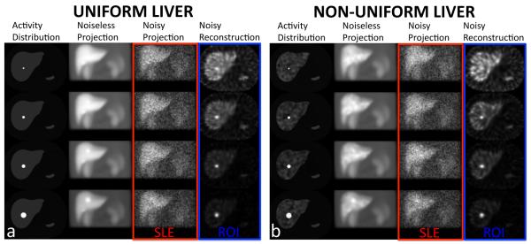
We generated NCAT activity and attenuation phantoms (matrix size: 256×256×256 and voxel size: 0.2332 cm). In the activity phantom, we added spherical tumors of varying diameters (1, 1.5, 2 and 3 cm) and contrast ratios (1-10, with increments of 1) to the liver. The coefficients of the attenuation phantom were based on the 171 keV emission photons of ¹¹¹In radionuclide only, and the 245 keV emission was not considered. Projections were obtained over 120 angles covering 360 degrees around the phantom using an analytical projector modeling a dual-head general-purpose clinical SPECT scanner. The photon attenuation and distance-dependent collimator blurring (parallel-hole medium-energy collimator) were included in the projector model. The production of scattered photons was not included. The 256×256×120 projection data were downsized to 128×128×120 and scaled to ~ 5 million total counts, which represented the count level in ¹¹¹In-Octreotide SPECT studies. These voxel values were used as the means for generating 100 Poisson-distributed independent noise realizations for each tumor size and contrast ratio (CR). The SLE method operated on these projection datasets, and the ROI method operated on their reconstructions using an iterative reconstruction algorithm (OSEM: 5 iterations and 30 subsets) with attenuation correction, resolution compensation based on modeling of the 3D spatial resolution and without post-filtering (P H Pretorius et al 1998). In figure 1a, slices from the activity distribution, projection, and reconstruction are shown for 4 tumor sizes at CR=5 added to the uniform background, which represents an ideal background condition. Such a situation is referred as “background known exactly” (BKE) in the literature (H H Barrett et al 1993). A total of 4000 independent noisy projection datasets were obtained (4 tumor sizes × 10 tumor activity levels × 100 Poisson noise realizations) from these phantoms with uniform liver background. In figure 1b, slices are shown for the non-uniform background, which represented a more realistic background condition referred to as “background known statistically” or BKS (S Young et al 2009) obtained by randomly superimposing Gaussian functions upon the uniform background forming “Lumpy objects” as described in (J P Rolland and H H Barrett 1992). In this way, we created 4000 independent nonuniform liver backgrounds (100 samples for each tumor size and activity level). Each of these phantoms was then projected and Poisson noise added. Therefore, as in the case of the uniform background, 4000 (100 white noise × 4 tumor sizes × 10 tumor activity levels × 1 Poisson noise realization) noisy projections were obtained for the nonuniform background. We defined the parameters of the 3D Gaussian such that the lumpy texture is as dominant as possible while keeping the object pixel values positive. Therefore the non-uniform liver background ranged from zero to twice the uniform background.

Figure 1.

Sample transverse slices of the activity distributions, noise free and noisy anterior projections (1 out of 120 total projections), and transverse reconstructions of the NCAT phantom. Spherical simulated tumors of 1, 1.5, 2 and 3 cm diameters (1^st row – 4^th row) for a contrast ratio (CR) of 5 inserted into (a) uniform liver and (b) non-uniform liver backgrounds, are shown. Note as indicated in the figure, the SLE and ROI methods operate on the raw projection and reconstruction data, respectively.

2.2 Region of Interest (ROI) Estimation from the Reconstructed Data

The activity distribution of the object is a square-integrable function of a continuous spatial variable f(r; α) = αχ_sig (r) + f_bkg (r). Here the tumor activity α is in units of activity/volume, f_bkg (r) denotes the background activity, and χ_sig (r) is a unitless support function that specifies the location and shape of the tumor and is equal to one at all points within the tumor volume and zero everywhere else. By rearranging terms in the activity distribution of the object, the tumor activity concentration can be expressed as $\alpha ={\left(\mathbf{f}\right(\alpha )-{\mathbf{f}}_{\text{bkg}},{\chi }_{\text{sig}})}_{{\mathbb{R}}^3}∕{({\chi }_{\text{sig}},{\chi }_{\text{sig}})}_{{\mathbb{R}}^3}$, which is an inner product in the Hilbert space $L_2\left({\mathbb{R}}^3\right)$.

The inner product between continuous functions is replaced by a discrete sum when the continuous object is represented by a discrete reconstruction. Then the ROI estimator of activity concentration can be written as, ${\widehat{\alpha }}_{\mathrm{ROI}}={(\mathbf{F}-{\mathbf{F}}_{\text{bkg}},X_{\text{sig}})}_{{\mathbb{E}}^N}∕{(X_{\text{sig}},X_{\text{sig}})}_{{\mathbb{E}}^N}$, where F is an N-voxel reconstruction of the object and F_bkg is a reconstruction of just the background portion of the object. This estimation rule for the ROI method requires prior values for the location and shape of the tumor to calculate the template X_sig that forms an inner product with the reconstruction. In this paper X_sig will be referred to as the tumor template for the ROI estimator. Our simulation study includes perturbing this prior knowledge away from the true value as detailed in section 2.5.

2.3 Scanning Linear Estimation (SLE) from the Raw Projection Data

The SLE estimation rule for the activity concentration in a tumor, adopted by M K Kupinski et al (2013), can also be written as an inner-product but in projection data instead of reconstructed images:

$${\widehat{\alpha }}_{\mathrm{SLE}}\left(\mathbf{g}\right)=\frac{({\mathbf{sK}}_{\mathbf{g}\mid \overline{\alpha }}^{-1∕2},(\mathbf{g}-\overline{\mathbf{b}}\left){\mathbf{K}}_{\mathbf{g}\mid \overline{\alpha }}^{-1∕2}\right)}{({\mathbf{sK}}_{\mathbf{g}\mid \overline{\alpha }}^{-1∕2},{\mathbf{s}}^{\prime }{\mathbf{K}}_{\mathbf{g}\mid \overline{\alpha }}^{-1∕2})},$$

where g represents the noisy image measured by the imaging system, $\overline{\mathbf{b}}$ is a noise-free image of the average background, ${\mathbf{K}}_{\mathbf{g}\mid \overline{\alpha }}^{-1}$ is the inverse of the conditional data covariance matrix given $\overline{\alpha }$ (the average value of the tumor activity), and s is the noise-free image of χ_sig (r) describing the tumor location and shape in the projection space. In this paper χ_sig (r) will be referred to as the tumor template for SLE. To obtain $\mathbf{s}=\mathcal{H}{\chi }_{\mathit{sig}}\left(\mathbf{r}\right)$, an accurate forward projection operator $\mathcal{H}$ modeling the imaging system (including attenuation and system resolution), is required.

Multiplying an image with a data covariance matrix to the one-half power, such as ${\mathbf{g}}^{\mathit{PW}}={\mathbf{K}}_{\mathbf{g}}^{-1∕2}\mathbf{g}$, is referred to as pre-whitening since the resulting image will have a variance equal to one for every pixel and each pixel will be uncorrelated with other pixels, i.e. K_g^PW is the identity matrix (H H Barrett and K J Myers 2004). Notice that the SLE uses a conditional data covariance matrix so that the matrix-vector product is only exactly pre-whitening when the true value for the tumor activity equals the average value. The SLE computation can be summarized as performing an approximation to pre-whitening in the raw projection domain and forming an inner-product in that domain between the modeled and measured data.

2.4 Evaluating the Data Covariance: Weak Signal Approximation in the Noise Term

In this simulation study we consider the image randomness due to both Poisson measurement noise and fluctuations in the background due to population statistics. To simulate an unknown background activity distribution, a random texture is generated in the NCAT liver as explained in section 2.1. These effects are modeled in the SLE by using the two terms found when analyzing the covariance decomposition ${\mathbf{K}}_{\mathbf{g}\mid \overline{\alpha }}={\mathbf{K}}_{\mathbf{n}\mid \overline{\alpha }}+{\mathbf{K}}_{\mathbf{b}}$ (H H Barrett and K J Myers 2004) and (A Könik et al 2014). It should be noted that the covariance decomposition is an exact expression and does not rely on any assumptions. The background covariance K_b does not depend upon the signal but the noise term ${\mathbf{K}}_{\mathbf{n}\mid \overline{\alpha }}$ is conditioned on the average value of the signal, therefore $\overline{\alpha }$ appears in the conditional notation. In practice the contribution of the signal to the conditional covariance matrix is usually small compared to other contributions: the background fluctuations described by K_b and the average background value that populates K_n . We have found that using the signal absent conditional data covariance matrix, K_g∣α=0 = K_n∣α=0 + K_b , in place of the data covariance matrix conditioned on the average signal does not change SLE performance for this simulation study. The advantage of this substitution is that a value for $\overline{\alpha }$ is no longer required to evaluate the conditional covariance used in the SLE calculation. Therefore, we used K_g∣α=0 for all the SLE results presented in this paper.

2.5 Inverting the Data Covariance: Background Known Statistically (BKS) in a Compact Region

For BKS, the noise term is diagonal for the projection images but the background covariance K_b is not (for BKE K_b = 0 , thus the conditional data covariance matrix is diagonal). The off-diagonal terms complicate the computation of the matrix inverse. The background covariance is written in object space so that the spatial support of the liver can be used to simplify the matrix inverse, ${\mathbf{K}}_{\mathbf{g}\mid \alpha =0}={\mathbf{K}}_{\mathbf{n}\mid \alpha =0}+{\mathcal{HK}}^{\mathit{bkg}}{\mathcal{H}}^{†}$ , where the imaging operator $\mathcal{H}$ relates the object covariance operator ${\mathcal{K}}^{\mathit{bkg}}$ to the image covariance matrix K_b . If the heterogeneous activity in the liver is assumed to be isotropic and stationary, then the background covariance kernel function is K^bkg (r,r′) = S^liver (r)S^liver (r′)γ(∣r − r′∣), where S^liver (r) is a binary function denoting the spatial support of the liver and γ (∣r − r′ ∣) is the stationary covariance function that determines the statistical fluctuations. Then ${\mathbf{K}}_{\mathbf{g}\mid \overline{\alpha }}^{-1}\mathbf{s}$ can be estimated using an iterative relation ${\widehat{\mathbf{w}}}_{n+1}={\widehat{\mathbf{w}}}_n+ϵ{\left[{\mathbf{K}}_{\mathbf{n}\mid \alpha =0}\right]}^{-1}[\mathbf{s}-{\mathbf{K}}_{\mathbf{g}\mid \alpha =0}{\widehat{\mathbf{w}}}_n]$ (H H Barrett and K J Myers 2004), where ϵ scales an additive update term. This update term tends to zero as the residual $\mathbf{s}-{\mathbf{K}}_{\mathbf{g}\mid \alpha =0}{\widehat{\mathbf{w}}}_n$ tends to an image of all zero entries. Substituting the two terms for the conditional data covariance matrix leads to ${\widehat{\mathbf{w}}}_{n+1}={\widehat{\mathbf{w}}}_n+ϵ{\left[{\mathbf{K}}_{\mathbf{n}\mid \alpha =0}\right]}^{-1}[\mathbf{s}-{\mathbf{K}}_{\mathbf{n}\mid \alpha =0}{\widehat{\mathbf{w}}}_n-{\mathcal{HK}}^{\mathit{bkg}}{\mathcal{H}}^{†}{\widehat{\mathbf{w}}}_n]$, where the utility of this expression is that an inverse of the non-diagonal portion of the covariance matrix is not required. In this work we found convergence of this iterative algorithm at around 100 iterations. As expected, the number of iterations depended most strongly on the magnitude of the background covariance term. A more detailed discussion of this iterative technique is given near Equation 14.36 of Barrett & Myers Foundations of Image Science.

2.6 Comparison of Estimation Performance

We compared the performance of the ROI and SLE estimates of tumor activity concentration $\widehat{\alpha }$ by using the ensemble mean-square error (EMSE) as the task-performance criterion. First, the mean square-error $\mathrm{MSE}(\widehat{\alpha },\alpha )=<{(\widehat{\alpha }-\alpha )}^2{>}_{\mathbf{g}\mid \alpha }$ was obtained from 100 independent samples for each tumor size and contrast ratio. Then EMSE was calculated as $\mathrm{EMSE}\left(\widehat{\alpha }\right)=<\mathrm{MSE}(\widehat{\alpha },\alpha ){>}_{\alpha }$ , where MSE was averaged over 10 tumor contrast ratios. For each tumor size and activity level, standard deviations (SD) of the ROI and SLE estimations were also obtained.

We investigated three different levels of prior knowledge:

1) When the tumor location, shape and size were modeled accurately. For this ideal case, we simulated two different tumor locations, one close to the edge of the liver (figure 2a) and the other one close to the center of the liver (figure 2b), to observe how the estimations depend on the location. These tumors were ~ 6 cm (x: 2.3 cm, y: 5.4 cm, z: 1.4 cm) apart from each other. The rest of the estimations were based on the tumor close to the center, only.

Figure 2.

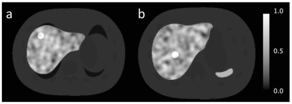
Two different locations are shown for the 2 cm tumor with the lowest contrast ratio of 1: (a) close to the edge of the liver and (b) close to the center of the liver.

2) When the tumor shape and size were modeled accurately, but the modeled tumor location was not correct. This simulated a potential mistake in centering the lesion. In this case, the SLE and ROI calculations were performed deliberately at 1 pixel (0.4664 cm) and 2 pixels (0.9328 cm) away from the actual tumor location in projection and reconstruction spaces. To calculate the activity estimates using this incorrect model, the tumor locations are shifted in the tumor template χ_sig for SLE and the tumor template X_sig for ROI.

3) When the tumor location was modeled accurately, but the modeled tumor size was not correct. This simulated a potential mistake in the measurement size. In this case, the SLE and ROI calculations were performed deliberately using smaller and larger template volumes ranging from −50% to +50%.

All the measurements described above were performed for both uniform and non-uniform backgrounds using the EMSE as the criterion.

Results

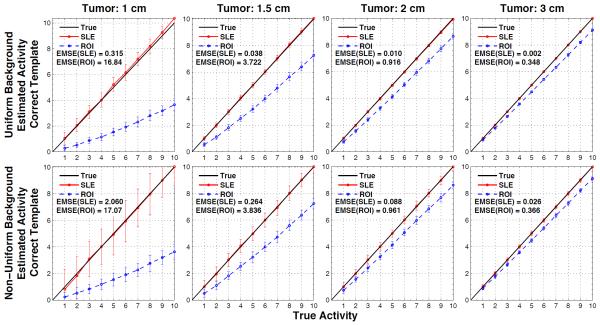
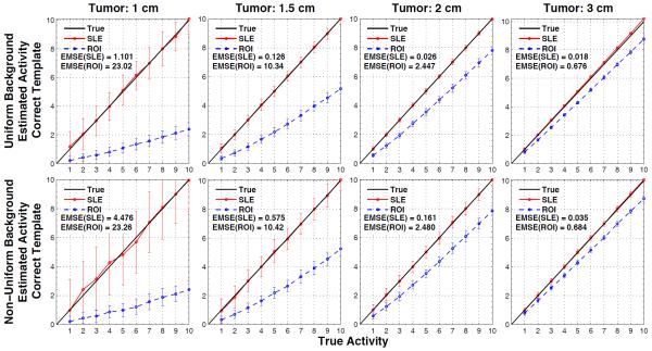
The estimation performance of the ROI and SLE methods for the ideal case are shown in figures 3 and 4 for the tumors located close to the liver edge (figure 2a) and the liver center (figures 2b), respectively. In both figures, the plots show the estimated versus true activity and EMSE values for the 4 tumor sizes investigated for the ROI and SLE estimation methods. The 1^st row of plots in these figures is for the case of uniform background and the 2^nd row is for the case of non-uniform background in the liver. Each plot shows the mean estimated activity concentrations and their SD as bars about the mean values at 10 different contrast ratios increasing from left to right for a given tumor size. By its much lower EMSE results it can be noted that the SLE method dramatically outperformed the ROI method for both background conditions. This can also be seen from the activity estimations of SLE being well aligned with the true activity line, thus showing no bias. On the other hand, ROI estimations were below the true activity line (i.e., underestimated) and the amount of bias depended on the tumor size, activity and location. Comparison of ROI estimations in figures 3 and 4 show the bias introduced by tumor location. For example, the slopes for ROI estimations in figure 3 are about double that of figure 4 for the 1 cm tumor. Hence, a constant correction factor cannot be applied to all ROI estimates to compensate for the bias introduced by the ROI estimator. For the non-uniform background, the magnitude of the bias of both estimators was approximately unchanged, however, the SD of the SLE increased more than the ROI’s SD. Nevertheless, the normalized SLE(SD) values are still smaller (except for few cases) than the ROI(SD) as explained in the discussion section.

Figure 3.

Results for when the tumor size and location are known exactly, for tumors at location of figure 2a. Average SLE and ROI estimated activities are plotted relative to the true activities for the uniform liver (1^st row) and non-uniform liver (2^nd row) backgrounds. The error bar for each data point is the standard deviation over 100 noise realizations. As indicated by the ensemble mean-square errors (EMSE), SLE dramatically outperformed ROI for all these cases.

Figure 4.

Results for when the tumor size and location are known exactly, for tumors at location of figure 2b. Average SLE and ROI estimated activities are plotted relative to the true activities for the uniform liver (1^st row) and non-uniform liver (2^nd row) backgrounds. The error bar for each data point is the standard deviation over 100 noise realizations. As indicated by the ensemble mean-square errors (EMSE), SLE dramatically outperformed ROI for all these cases. Differences in the ROI slops between the figure 3 and 4 show how ROI estimation is biased by the tumor location.

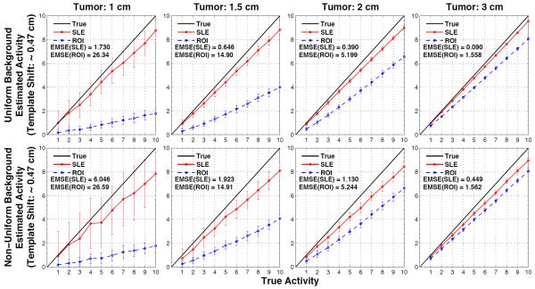
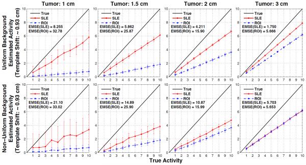
Figures 5 and 6 show the estimated versus true activities when the volumes used by the SLE and ROI estimators were deliberately perturbed 0.4664 cm (figure 5) or 0.9328 cm (figure 6) away from the actual tumor location. Again the 1st row of plots in these figures is for the case of uniform background and the 2nd row is for the case of non-uniform background in the liver. As expected with incorrect template location SLE becomes biased, underestimating the true activity values since the lower pixel values from the background replaced the higher pixel values in the tumor. Similarly, ROI estimations further underestimated. The increase in SLE(EMSE) with incorrect template location is much larger than ROI(EMSE), especially for larger tumor sizes. For example, for the 3 cm tumor added to the non-uniform background SLE(EMSE) and ROI(EMSE) increases are ~ 13 and ~ 2 fold, respectively. At 2 pixels shift from the actual tumor location, ROI estimations further approach the SLE estimations. In fact, for the 3 cm tumor added to the non-uniform background (figure 6, right bottom corner), the estimates are almost the same although EMSE(ROI) becomes slightly lower than EMSE(SLE).

Figure 5.

Results for when the tumor size is known but the location of the tumor model employed in SLE and ROI estimation is shifted by 1 pixel (~ 0.47 cm) from the correct location of the tumor (as displayed in figure 2b). Average SLE and ROI estimated activities are plotted relative to the true activities for the uniform liver (1^st row) and non-uniform liver (2^nd row) backgrounds. The error bar for each data point is the standard deviation over 100 noise realizations. As indicated by the ensemble mean-square errors (EMSE), SLE dramatically outperformed ROI for all these cases.

Figure 6.

Results for when the tumor size is known but the location of the tumor model employed in SLE and ROI estimation is shifted by 2 pixels (~ 0.93 cm) from the correct location of the tumor (as displayed in figure 2b). Average SLE and ROI estimated activities are plotted relative to the true activities for the uniform liver (1^st row) and non-uniform liver (2^nd row) backgrounds. The error bar for each data point is the standard deviation over 100 noise realizations. ROI estimations approach the SLE estimations compared to the case of 1 pixel off. For the 3 cm tumor added to the non-uniform background (right bottom corner), SLE and ROI estimations are about the same.

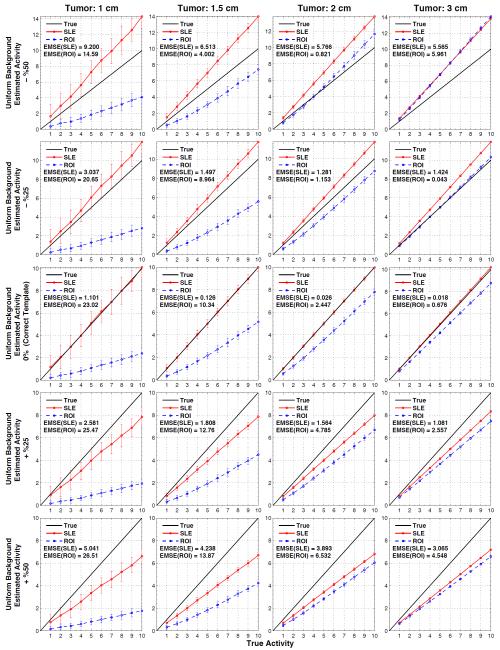
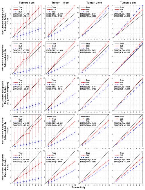
Figure 7 shows the estimated versus true activity for uniform background when tumor sizes are not accurately known and figure 8 does this for the non-uniform background. The actual tumor sizes are indicated on top of each column and the errors in the modeled tumor volume are indicated in the vertical axis of the plots: −50%, −25%, 0%, +25%, and +%50 for the 1^st - 5^th rows, respectively. Therefore, the plots in the middle row are obtained by using the correct measurement sizes (and correct locations), and hence they are the same plots as in figure 4.

Figure 7.

Results for when the tumor location (as displayed in figure 2b) is known but the size of the tumor model employed in SLE and ROI estimation is inaccurate (errors in volumes: ±%50). Average SLE and ROI estimated activities plotted relative to the true activities for the uniform background. Plots in the middle row are for the ideal cases (figure 4, 1^st row), where the correct tumor model (both size and location) is used.

Figure 8.

Results for when the tumor location (as displayed in figure 2b) is known but the size of the tumor model employed in SLE and ROI estimation is inaccurate (errors in volumes: ±%50). Average SLE and ROI estimated activities plotted relative to the true activities for the non-uniform background. Plots in the middle row are for the ideal cases (figure 4, 1^st row), where the correct tumor model (both size and location) is used.

In all the plots presented in figure 7 and figure 8, both SLE and ROI activity concentration estimations decrease with the increasing template volume. This trend is expected as more counts are recorded at the center of the tumor and increasing the template volume decreases the estimation of activity concentration. Since SLE is an unbiased estimator (when correct template is in use), smaller templates result in overestimation and larger templates in underestimation. These errors decrease as the template size approaches the tumor size (−25% or +25%). Also, EMSE(SLE) values obtained with +50% were lower than that of −%50 because of better count statistics (lower SD) within the larger template volume. On the other hand, the ROI estimations were not as predictable since they are biased even with the correct templates. For example when −50% template is used, activities in tumors of 1cm and 1.5 cm were underestimated whereas activities in tumors of 2 cm and 3 cm were overestimated. Because of the trend explained above, in some cases ROI estimations became closer to the true line. For example, the activity concentration of the 3 cm tumor was better estimated with a −25% template than using a correct template.

Figure 7 and Figure 8 demonstrate that SLE performed better than ROI in estimating the activity concentration of the 1 and 1.5 tumors for all the templates. For the 2 cm and 3 cm tumors, ROI “appeared” to estimate better than SLE for a few cases for the reasons explained above.

Discussion

We presented here an extensive comparison of the SLE and ROI methods under different conditions. The variables of this study were: 4 tumor sizes, 10 tumor activities, 2 tumor locations, uniform and non-uniform liver backgrounds and 3 different assumptions about the knowledge of tumor location and size. While our results are based on the estimation of activity concentration, the plots presented in figure 3-6 and figure 9 apply to the uptake estimation also, by simply scaling them with the respective tumor volumes. For the figures 7 and 8 a direct scale cannot be applied since the actual tumor and template volumes were not the same. Nevertheless, the opposite of the general trend for the activity concentration estimation would be true for the uptake estimation. That is, both SLE and ROI uptake estimations would increase with the increasing template volume.

Figure 9.

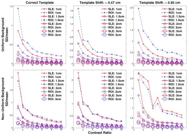
SD(estimation)/mean(estimation) values plotted for the 10 contrast ratios (CR) and 4 tumor sizes for the uniform (1^st row) and non-uniform liver (2^nd row) backgrounds. The sizes of the data markers are proportional to the tumor sizes. For the ideal case (using the correct tumor model), the relative SLE variances are lower than that of ROI for all marker sizes and CR. When the modeled tumor location is shifted, relative SLE variances are lower and only slightly larger than that of ROI for the uniform and non-uniform liver, respectively.

Our simulation results showed that the activity estimation performance of the unbiased SLE method was much better than that of the ROI method, especially under ideal conditions when the tumor location and size are modeled accurately. For this ideal case, we simulated tumors in two different locations to see the location dependency of the estimations. The photon emission from the tumor deeper in the body (figure 2b) was attenuated more compared to the photons emitted by the tumor close to the liver boundary (figure 2a) resulting in larger uncertainty in the count distribution and errors in estimations. In fact, all the EMSE results obtained from the tumor deeper in the body (figure 4) were larger than the ones obtained from the tumor close to the liver boundary (figure 3). The comparison of two figures also showed that ROI estimations were biased depending on the location of the tumor while SLE estimations remained unbiased. All the results shown in figure 4-9 were obtained from the tumor deeper in the body.

Assuming a uniform background and accurate knowledge of tumor size and location is an oversimplification. For this reason, as a more realistic background condition we considered the non-uniform liver activity and also performed the estimation tasks when tumor location or size are inaccurately known. While the SLE method was more sensitive to the usage of such inaccurate knowledge it still performed considerably better than the ROI method.

EMSE results showed the combined error from the SD and bias since EMSE = < SD² + Bias² >_CR. However, the individual impacts of SD and bias are also important. The plots clearly show that SLE provides unbiased estimations for the ideal case and less biased estimations compared to ROI’s when the template model is not accurate. On the other hand, SD bars displayed on the plots are larger for SLE mainly because the estimations obtained from SLE are larger than the ROI estimations, which may lead to misinterpretation of these results. A more relevant comparison of these two methods is to use normalized SD values: SD_norm= SD(estimations) / mean(estimations). In figure 9, we show these results for the 10 contrast ratios and 4 tumor sizes for the uniform (1^st row) and non-uniform liver (2^nd row) backgrounds. These normalized SD plots show that, when a correct template is used, the relative SLE variances are lower than that of ROI for all marker sizes and contrast ratios with few exceptions in the non-uniform case. When the tumor template location is shifted, relative SLE variances are lower and only slightly larger than that of ROI for the uniform and non-uniform liver, respectively. These results confirm that SLE provides unbiased estimations while its variance is still better or comparable to that of ROI.

The 5 million total counts used in the simulated projections for ¹¹¹In- Octreotide imaging was based on that of clinical acquisitions at our site. However, one might expect the number of counts acquired to be less with larger patients or lower administered activity to reduce patient radiation dose. Thus we repeated the simulations of the phantoms with 2 cm tumor at 2.5 million count level to see how SLE and ROI methods compare at lower count levels. At this count level EMSE(SLE) increased by 6 fold and EMSE(ROI) remained essentially unchanged. Nevertheless, EMSE(SLE) remained to be 18 times lower than EMSE(ROI).

The results of this study indicated that the accuracy of the template size and location is critical for the performance of the SLE. This may be achieved by using the SLE method to its full potential by incorporating a size and location search in the raw projection data, as described in (M K Kupinski et al 2013). To further improve this approach and reduce the computation time, the location search can be performed in a smaller region by using the location information obtained from the SPECT reconstruction or registered CT scans if available.

Our results may suggest that a slightly smaller template size can help improving the ROI quantification if the reconstruction method tends to underestimate the activity concentration. However, one needs to be cautious in choosing the template size as smaller templates may result in overestimation and even larger errors. Such a choice would largely depend on the actual tumor size and the details of the reconstruction method apart from the other dependencies such as tumor activity and location. The opposite conclusions can be drawn for the uptake estimations where a slightly larger template may provide better ROI quantification.

In these studies we did not model the 245 keV photon emitted by ¹¹¹In, nor photon scattering in SPECT imaging to enable comparison of ROI and SLE under controlled conditions. Now that we have documented the superiority of the SLE methodology with this limited modeling of the physics of imaging there is motivation to investigate the relative quantification obtained from complete Monte Carlo modeling of all emitted photons during imaging, hybrid studies where one adds the tumor in actual clinical studies, and finally true clinical application.

Conclusion

We presented the simulation results of a ¹¹¹In-Octreotide SPECT study as a clinical application for the SLE method operating in the projection space in comparison to the conventional ROI method operating in the reconstruction space. We considered a large range of tumor sizes and activities added to uniform and non-uniform liver backgrounds under different assumptions about the knowledge of the tumor size and locations. The simulation results showed that the unbiased SLE method performs much better than the ROI method, especially when the tumor location and size are modeled accurately. Although SLE was impacted more than ROI method when a non-uniform background is used and the modeled tumor location was not accurate, SLE still continued to perform better than ROI.

REFERENCES

- Barrett HH. Objective assessment of image quality: effects of quantum noise and object variability. J Opt Soc Am A. 1990;7:1266–78. doi: 10.1364/josaa.7.001266. [DOI] [PubMed] [Google Scholar]
- Barrett HH, Myers KJ. Foundations of Image Science. Wiley-Interscience; New York: 2004. [Google Scholar]
- Barrett HH, Yao J, Rolland JP, Myers KJ. Model observers for assessment of image quality. Proc Natl Acad Sci U S A. 1993;90:9758–65. doi: 10.1073/pnas.90.21.9758. [DOI] [PMC free article] [PubMed] [Google Scholar]
- Carson RE. A maximum likelihood method for region-of-interest evaluation in emission tomography. J Comput Assist Tomogr. 1986;10:654–63. doi: 10.1097/00004728-198607000-00021. [DOI] [PubMed] [Google Scholar]
- Clarkson E, Barrett H. Bounds on null functions of linear digital imaging systems. Journal of the Optical Society of America. A, Optics, image science, and vision. 1998;15:1355–60. doi: 10.1364/josaa.15.001355. [DOI] [PubMed] [Google Scholar]
- Defrise M, Townsend D, Geissbuhler A. Implementation of three-dimensional image reconstruction for multi-ring positron tomographs. Phys Med Biol. 1990;35:1361–72. doi: 10.1088/0031-9155/35/10/002. [DOI] [PubMed] [Google Scholar]
- Huesman RH. A new fast algorithm for the evaluation of regions of interest and statistical uncertainty in computed tomography. Phys Med Biol. 1984;29:543–52. doi: 10.1088/0031-9155/29/5/007. [DOI] [PubMed] [Google Scholar]
- Kinahan PE, Fletcher JW. Positron emission tomography-computed tomography standardized uptake values in clinical practice and assessing response to therapy. Seminars in ultrasound, CT, and MR. 2010;31:496–505. doi: 10.1053/j.sult.2010.10.001. [DOI] [PMC free article] [PubMed] [Google Scholar]
- Könik A, Kupinski M, Pretorius P, King M, Barrett H. IEEE MIC. Seattle WA: 2014. Comparison of the Scanning Linear Estimator (SLE) and ROI Uptake Estimation for Quantitative 111In-Octreotide SPECT Imaging of Signals Embedded in Random Backgrounds. [Google Scholar]
- Kontogeorgakos DK, Dimitriou PA, Limouris GS, Vlahos LJ. Patient-specific dosimetry calculations using mathematic models of different anatomic sizes during therapy with In-111-DTPA-D-Phe(1)-octreotide infusions after catheterization of the hepatic artery. Journal of Nuclear Medicine. 2006;47:1476–82. [PubMed] [Google Scholar]
- Kupinski MK, Clarkson EW, Barrett HH. Scanning linear estimation: improvements over region of interest (ROI) methods. Phys Med Biol. 2013;58:1283–301. doi: 10.1088/0031-9155/58/5/1283. [DOI] [PMC free article] [PubMed] [Google Scholar]
- Moore SC, Southekal S, Park MA, McQuaid SJ, Kijewski MF, Muller SP. Improved regional activity quantitation in nuclear medicine using a new approach to correct for tissue partial volume and spillover effects. IEEE Trans Med Imaging. 2012;31:405–16. doi: 10.1109/TMI.2011.2169981. [DOI] [PMC free article] [PubMed] [Google Scholar]
- Muller SP, Kijewski MF, Moore SC, Holman BL. Maximum-likelihood estimation: a mathematical model for quantitation in nuclear medicine. J Nucl Med. 1990;31:1693–701. [PubMed] [Google Scholar]
- Park MA, Moore SC, Muller SP, McQuaid SJ, Kijewski MF. Performance of a high-sensitivity dedicated cardiac SPECT scanner for striatal uptake quantification in the brain based on analysis of projection data. Med Phys. 2013;40:042504. doi: 10.1118/1.4794488. [DOI] [PMC free article] [PubMed] [Google Scholar]
- Pretorius PH, King MA, Pan TS, de Vries DJ, Glick SJ, Byrne CL. Reducing the influence of the partial volume effect on SPECT activity quantitation with 3D modelling of spatial resolution in iterative reconstruction. Phys Med Biol. 1998;43:407–20. doi: 10.1088/0031-9155/43/2/014. [DOI] [PubMed] [Google Scholar]
- Razifar P, Sandstrom M, Schnieder H, Langstrom B, Maripuu E, Bengtsson E, Bergstrom M. Noise correlation in PET, CT, SPECT and PET/CT data evaluated using autocorrelation function: a phantom study on data, reconstructed using FBP and OSEM. BMC medical imaging. 2005;5:5. doi: 10.1186/1471-2342-5-5. [DOI] [PMC free article] [PubMed] [Google Scholar]
- Rolland JP, Barrett HH. Effect of random background inhomogeneity on observer detection performance. J Opt Soc Am A. 1992;9:649–58. doi: 10.1364/josaa.9.000649. [DOI] [PubMed] [Google Scholar]
- Schillaci O, Spanu A, Scopinaro F, Falchi A, Danieli R, Marongiu P, Pisu N, Madeddu G, Delle Fave G. Somatostatin receptor scintigraphy in liver metastasis detection from gastroenteropancreatic neuroendocrine tumors. J Nucl Med. 2003;44:359–68. [PubMed] [Google Scholar]
- Segars WP, Sturgeon G, Mendonca S, Grimes J, Tsui BM. 4D XCAT phantom for multimodality imaging research. Med Phys. 2010;37:4902–15. doi: 10.1118/1.3480985. [DOI] [PMC free article] [PubMed] [Google Scholar]
- Southekal S, McQuaid SJ, Kijewski MF, Moore SC. Evaluation of a method for projection-based tissue-activity estimation within small volumes of interest. Phys Med Biol. 2012;57:685–701. doi: 10.1088/0031-9155/57/3/685. [DOI] [PMC free article] [PubMed] [Google Scholar]
- Whitaker MK, Clarkson E, Barrett HH. Estimating random signal parameters from noisy images with nuisance parameters: linear and scanning-linear methods. Opt Express. 2008;16:8150–73. doi: 10.1364/oe.16.008150. [DOI] [PMC free article] [PubMed] [Google Scholar]
- Young S, Park S, Anderson SK, Badano A, Myers KJ, Bakic P. Estimating breast tomosynthesis performance in detection tasks with variable-background phantoms. 2009:72580O–80O-9. [Google Scholar]