Survival analysis in hematologic malignancies: recommendations for clinicians

Abstract

The widespread availability of statistical packages has undoubtedly helped hematologists worldwide in the analysis of their data, but has also led to the inappropriate use of statistical methods. In this article, we review some basic concepts of survival analysis and also make recommendations about how and when to perform each particular test using SPSS, Stata and R. In particular, we describe a simple way of defining cut-off points for continuous variables and the appropriate and inappropriate uses of the Kaplan-Meier method and Cox proportional hazard regression models. We also provide practical advice on how to check the proportional hazards assumption and briefly review the role of relative survival and multiple imputation.

Introduction

In clinical research, the main objective of survival analysis is to find factors able to predict patient survival in a particular clinical situation. Ideally, we should be able to develop an accurate and precise prognostic model incorporating those clinical variables that are most important for survival. Survival methods are very popular among statisticians and clinicians alike, relatively easy to perform, and available in a variety of statistical packages. However, we have observed that these powerful tools are often used inappropriately, perhaps because most papers or books dealing with statistical methods are written by statisticians (not surprisingly!), and these texts could be daunting for clinicians who only wish to know how to run a particular test and are not particularly interested in the theory behind it. Ideally, statistical analyses should be performed by statisticians. But it is not always easy for investigators to find statisticians with a specific interest in survival analysis. Consequently, it is advisable to have a sound grasp of several statistical concepts in case we ever decide to do our own statistical analysis.

The purpose of this review is to identify mistakes commonly observed in the literature and provide ideas on how to solve them. In order to illustrate some of the ideas presented, we will use our institution’s database of patients with chronic lymphocytic leukemia (CLL), which has been prospectively managed for more than 30 years.¹ We will also provide examples computed using several statistical packages of our liking: Stata (StataCorp, Texas, USA), SPSS (IBM, New York, USA) and R software environment. The first two packages are available in many institutions worldwide, but at a considerable cost (even though Stata is relatively inexpensive compared to SPSS). R, on the other hand, is freely available at www.r-project.org. Of note, R performs many basic statistical tests and the website provides additional packages for specific purposes, all of which are also free, but it does require some basic programming skills.

We are not statisticians but hematologists, and we have tried to simplify the statistical concepts as much as possible so that any hematologist with a basic interest in statistics can follow our line of reasoning. By doing so, we might have inadvertently used some expressions or mathematical concepts inappropriately. We hope this is not the case, but we have purposefully avoided the help of a statistician because we did not want to write yet another paper full of equations, coefficients and difficult concepts that would be of little help to the average hematologist. On the other hand, we have a very high respect for statisticians, present and past, and we are very grateful to them. We have sought their advice many times, particularly when dealing with difficult concepts. However, we are also very realistic and, unfortunately, they cannot sit beside us every time we want to analyze our data.

ROC curves versus maximally selected rank statistics

Very often, an investigator wishes to evaluate the prognostic impact of a continuous variable (e.g. beta₂-microglobulin [β2M] concentration) on the survival of a series of patients with a particular disease (e.g. CLL), but does not know the cut-off value with the greatest discrimination power. The classic approach to this problem would be to plot a receiver operating characteristic (ROC) curve and then choose the cutoff value that is closest to the point of perfect classification (100% sensitivity and 100% specificity). Before doing that, the investigator needs to transform the time-dependent end point (survival) into a binary end point that is clinically relevant (e.g. survival at 3 years) and, therefore, only patients who have minimum of 3 years of follow up or who died within three years can be used in that analysis. Once the dataset is ready, we can plot the ROC curve and decide the most appropriate cut-off point, which is always a trade-off between sensitivity and specificity since the point of perfect classification does not exist in real life.

An interesting alternative is provided by maximally selected rank statistics.² This test can be easily applied using R (maxstat package) and has several advantages. First, there is no need to transform the time-dependent end point. Second, the test calculates an exact cut-off point, which can be estimated using several methods and approximations, and the discrimination power is also evaluated and estimated with a P value (type I error). Once you get the exact value (e.g. 2.3 mg/L), it is important to see if it is clinically relevant. For instance, in our institution, the upper limit of normality (ULN) for β2M is 2.4 mg/L, and we therefore decided to use 2.4 instead of 2.3 in order to avoid over-fitting the data. The idea behind this concept is that the investigator should look for a value that is clinically relevant (e.g. ULN, 2xULN, 3xULN) and easily applicable to a different patient population, and not the cut-off point that best describes the investigator’s own patient cohort.

Kaplan-Meier versus cumulative incidence curves

Kaplan-Meier (KM) estimates are commonly used for survival analysis and identification of prognostic factors, and the reason is that it is possible to analyze patients irrespective of their follow up.^3–5 Procedures for calculating KM estimates in R, Stata and SPSS are shown in Table 1. A very important aspect of these methods is that they ‘censor’ patients who had not experienced the event when they were last seen. As a result, these tools are appropriate when we wish to evaluate the prognostic impact of, for example, the IGHV mutation status on the overall survival of patients with CLL (Figure 1). They are also appropriate for other survival end points, such as disease-free or progression-free survival (Table 2).⁵ Several tests are available for comparing different KM estimates, of which the log rank test is the most popular.⁶

Table 1.

Procedures for survival analysis in R, Stata and SPSS.

Figure 1.

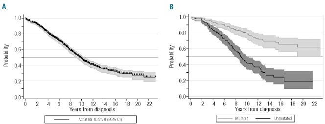
(A) Overall, projected survival (± 95% confidence interval) of our population of patients with chronic lymphocytic leukemia estimated according to Kaplan-Meier actuarial method. (B) Projected, actuarial survival (± 95% confidence interval) according to the IGHV genes mutational status (log rank test; χ² = 58.3; P<0.001). These curves were plotted using Stata (version 11.0).

Table 2.

Survival end points.

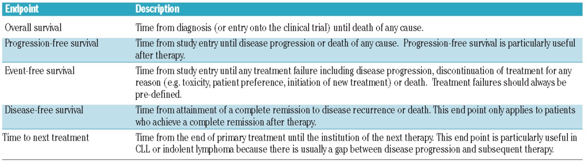
A disadvantage of these methods is that they only consider one possible event: e.g. death in case of overall survival, progression or death in case of progression-free survival, etc. (Table 2). However, in some diseases with an indolent course, such as CLL, it is not always feasible to use overall survival (OS) as the end point of the analysis since the median OS of patients with CLL is approximately ten years. Accordingly, investigators worldwide have frequently used other end points such as time to first treatment (TTFT) as a surrogate for disease aggressiveness.^7–10 Most investigators calculate TTFT using the inverse of a KM (1-KM) plot, but a problem arises in those patients who die before requiring any therapy. Since KM estimates only consider one possible event, the only option remaining is to censor these patients at the time of death, and this is never adequate. As a general rule, an observation is censored when the event of interest is not observed during the follow-up period, but the patient is still at risk of the event, which might occur at some unknown time in the future.⁵ If we think about the previous example, it is quite obvious that patients who die before requiring therapy are not at risk of requiring therapy in the future and are, therefore, incorrectly censored. To solve this problem, cumulative incidence curves that account for competing events are recommended.¹¹ Competing events refer to a situation where an individual is exposed to two or more causes of failure. Moreover, the statistical significance of a prognostic factor can be equally calculated, but Gray’s test must be used instead of the log rank test.¹² In the hematology field, these statistical tools have been developed mostly by investigators interested in hematopoietic transplantation because competing events are very common in that clinical scenario. For instance, transplant-related mortality and disease relapse are competing events that are commonly evaluated in patients undergoing transplantation. In general, few statistical packages offer simple ways of plotting cumulative incidence curves, but R is one of them, thanks to the cmprsk package (Table 1), which was, by the way, developed by Gray himself. Moreover, Scrucca et al. have published a highly recommended ‘easy guide’ that is not only useful for analyzing competing events or plotting cumulative incidence curves, but also as an initial introduction to R for investigators who have never used it before.¹³ The authors also wrote an R function called CumIncidence.R that can be freely downloaded from the University of Perugia’s website (http://www.stat.unipg.it/luca/R) and simplifies the analysis even further.

In the following example, we show how these different statistical tools could give different results. In our CLL database, we estimated the TTFT at five and ten years of our patient population according to age at diagnosis. Using the KM method, TTFT at five years was 53% for patients under 70 years of age and 38% for patients aged 70 years or older. When we considered death before therapy as a competing event, the results for patients younger and older than 70 years were 52% and 34%. The difference was negligible in younger patients (53 vs. 52%), but slightly higher for older patients (38 vs. 34%), the reason being that CLL-unrelated deaths were significantly more common in older patients. At ten years, however, the difference was higher because the degree of overestimation in older patients was significantly higher (51% by KM, 42% by cumulative incidence) compared to younger patients (64% vs. 62%). The final result is that in our patient population, there was a significant difference in 10-year-TTFT across both age groups: 13% using KM and 20% using cumulative incidence (P<0.001 for both tests) (Figure 2).

Figure 2.

(A) Time to first treatment in patients according to age (< 70 vs. ≥ 70 years) calculated using 1-KM curves (log rank test, χ² 14.1, P<0.001); and (B) cumulative incidence curves (Gray’s test, P<0.001). In panel B, deaths before therapy are considered as a competing risk. These curves were plotted using Stata (version 11.0).

A second example comes from a different area of hematology: thrombosis and hemostasis. Since venous thromboembolic events are clearly associated with cancer, there is considerable interest in defining risk factors for thrombosis and the role of anticoagulants in the management of cancer patients.¹⁴ However, a significant proportion of patients analyzed in these studies eventually die of their underlying malignancy before experiencing any thromboembolic event. A large number of clinical trials, some of them published in very prestigious journals,^15,16 have traditionally evaluated these cohorts using KM estimates, thus failing to account for deaths unrelated to thrombosis as a competing risk. Campigotto et al. analyzed these studies and concluded that KM analysis was inappropriate because the incidence of thrombosis was clearly over-estimated.¹⁷ Fortunately, things are changing in this field as well, and researchers participating in a more recent randomized trial used cumulative incidence instead of KM estimates.¹⁸

Evaluating covariates in survival analysis: don’t forget to set the clock on time!

Whenever we evaluate survival it is important to pay attention to the moment when we initiate follow up. As a general rule, the start time (time zero) is the first occasion when the patient is at risk for the event of interest. In transplant studies, this moment is usually the date of transplantation (i.e. hematopoietic cell infusion), while in clinical trials it is the date of study inclusion. In other circumstances, however, time zero is the date of diagnosis. Be that as it may, it is essential that any analysis only uses the information known at time zero, and not any information which may become available in the future.

For example, imagine that we would like to compare survival between patients with CLL who responded versus those who did not respond to front-line therapy, and we also wish to perform a multivariate analysis incorporating other well-established prognostic factors, such as ZAP70 expression or cytogenetics. The first thing to do is select the appropriate group of patients for our analysis, which in this particular case should be “patients with CLL who have received therapy”. The second step should be to decide the start time of our study, which in our example must be the time of disease evaluation after therapy (not time of CLL diagnosis) since we would like to include the covariate “response to therapy” in our survival analysis. Once these adjustments are made, we can proceed with our survival analysis as usual. This method is considered adequate, but it also has its detractors, particularly when the covariate evaluated is “response to therapy”.^19,20 Indeed, this analysis is intrinsically biased because the length of survival influences the chance of a patient being classified into one group (responders) or the other (non-responders). In other words, patients who will eventually respond to therapy must survive long enough to be evaluated as responders, and patients who die before the first response evaluation are automatically included in the “non-response” group.

Mantel-Byar test

A valid way of tackling this problem was described in 1974 by Mantel and Byar.²¹ Using their method, time starts at the moment of therapy initiation, and all patients begin in the “non-response” arm. Those who eventually respond to therapy enter the “response” state at the time of response and remain there until death or censoring, and those who do not respond always remain in the “non-response” arm. This method removes the bias as patients are compared according to their response status at various periods during follow up. At our institution, one of us (CR) developed a program for this purpose more than 30 years ago that has been recently translated into R code and is available upon request (Table 1). To the best of our knowledge, the only statistical package currently able to compute the original Mantel-Byar results (observed and expected numbers for both responders and non-responders) is SAS, but using a macro created by Alan Cantor.²²

Despite being an old and almost forgotten method, many researchers believe that the Mantel-Byar method is appropriate in some specific situations. For instance, in studies comparing allogeneic hematopoietic transplantation with conventional chemotherapy as consolidation therapy for patients with acute myeloid leukemia, researchers have usually resorted to a “donor” versus “no donor” analysis for the reason mentioned above: a direct comparison is always biased because patients must survive long enough to be eligible for transplantation, while those who die during the induction period are always counted in the non-transplant arm.^23,24 However, there is increasing awareness that “donor” versus “no donor” comparisons are not really accurate. As such, these studies assume that if a sibling donor was identified the transplantation actually occurred, which may not be the case. On the other hand, patients who do not have a sibling donor, but have an unrelated donor, are always allocated to the “no donor” group. It is precisely in this kind of situation when the Mantel-Byar test may be useful.²⁵

Landmark analysis

An alternative to the Mantel-Byar test is the landmark analysis.^19,26 In this method, time starts at a fixed time after the initiation of therapy. This fixed time is arbitrary, but must be clinically meaningful. For instance, if therapy usually lasts six months and disease response is usually evaluated three months after the last course of therapy, then a possible landmark point could be nine months after therapy initiation. Moreover, the transplant literature has established Day 100 as a demarcation point for distinguishing early from late transplant-related events, and this is often the basis for landmark analyses in transplantation.

Patients still alive at that landmark time are separated into two response categories according to whether they have responded before that time, and are then followed forward in time to evaluate whether survival from the landmark is associated with patients’ response. Patients who die before the time of landmark evaluation are excluded from the analysis, and those who do not respond to therapy or respond after the landmark time are considered non-responders for the purpose of this analysis. The advantages of this method over the Mantel-Byar test are: 1) it has a graphical representation, which is a Kaplan-Meier plot calculated from the landmark time; and 2) it can be performed in any statistical software, only requiring recalculation of the “time” and “status” variable for each patient. Sometimes it becomes more complicated, because the time point cannot be pre-defined. For example, we were interested in the impact of acquired genomic aberrations (clonal evolution) on patients’ outcome.¹⁸ For this purpose, we chose a cohort of patients who had two cytogenetic tests, and compared those who acquired genomic aberrations with those who did not. The problem arose because the time from the first test and the second was not constant among patients and we believe that this time could be of interest (i.e. the longer the follow up, the higher the risk of clonal evolution). In this situation, you cannot simply choose the date of the first cytogenetic test as time zero, because you do not know at that time if the patient will develop clonal evolution or not in the future, and you cannot set the clock on the date of the second cytogenetic test because by doing so you would neglect important follow-up information. The appropriate solution to this problem would be to select the date of the first cytogenetic test as time zero and include “clonal evolution” as a time-dependent covariate in a Cox regression model. We will discuss the different properties of this regression model in a separate section of this manuscript.

Relative survival

We must always remember that people with hematologic malignancies can die of a variety of reasons apart from the malignancy itself, particularly because they tend to be of advanced age.^27,28 Moreover, it is well known that patients with CLL and other lymphoid malignancies, even those who have never received therapy, have an increased risk of developing a second primary malignancy.^29,30 As a result, a significant proportion of patients with hematologic malignancies die of causes that are unrelated to the disease, and the investigator could be interested in dissecting the mortality that is truly attributable to the disease from the observed crude mortality. One way of doing this could be through a cumulative incidence analysis considering as events only those deaths that are clearly related to the disease, and as competing events the remaining disease-unrelated deaths (please, do not use 1-KM curves and censor patients who die of unrelated medical conditions!!!). However, this approach is problematic because it is not always easy to decide if the cause of death of a particular patient is related or not to the disease under study. Continuing with the example of patients with CLL: are all infectious deaths CLL-related, even if the patient never received therapy¿ What about patients who died of lung cancer or myocardial infarction but whose CLL was “active” at the time of death¿ How should we define “active” or “inactive” CLL¿

There is, however, a very interesting alternative, which is to calculate the relative survival of our patient cohort. This method circumvents the need for accurate information on causes of death by estimating the excess mortality in the study population compared to the general population within the same country or state.³¹ As such, mortality estimates are generally taken from national life tables stratified by age, sex and calendar year, and these life tables are readily available free of charge at the Human Mortality Database (www.mortality.org) and other websites. The relative survival ratio is defined as the observed survival of cancer patients divided by the expected survival of a comparable group from the general population (Figure 3A). In other words, the expected survival rate is that of a group similar to the patient group in such characteristics as age, sex and country of origin, but free of the specific disease under study.³² It could be argued, however, that in reality, the population mortality estimates will also contain a proportion of deaths caused by the disease under study,³³ but this proportion is negligible when we are evaluating relatively uncommon diseases such as hematologic malignancies.³⁴

Figure 3.

(A) Relative survival as the quotient of observed survival and predicted survival in the general population matched to the patients by age, sex and year of diagnosis. (B) Actuarial survival (Kaplan-Meier) and (C) relative survival according to age at diagnosis (70 or younger vs. older than 70). These curves were plotted using Stata (version 11.0).

In order to compare relative survival across categories of patients and identify prognostic factors, we assume that the number of failures per period of time (e.g. excess deaths per year) follows a Poisson distribution, and then check the goodness of fit by estimating the deviance, which is a measure of how much our data depart from the theoretical distribution. Interestingly, a feature of Poisson distribution is that mean and variance (“dispersion”) are required to be the same. In real-life data, however, this condition is rarely met because dispersion often exceeds the mean, a phenomenon referred to as “overdispersion“. Overdispersion can result from the own nature of the survival data themselves, because a relevant covariate (e.g. stage or histology) has been omitted from the analysis, or because a strong interaction between variables has not been considered (e.g. age and tolerance to chemotherapy).³⁵ In cases where the deviance is too high, we can assume that the variance is proportional to the mean, not exactly equal to it, and include in the model a ‘scale parameter’ that bears this proportional factor. If the deviance is still large after such adjustment, we can try using a different distribution such as the negative binomial. Stata and R provide a number of generalized linear models that allow these kinds of analyses, but a relatively high degree of statistical expertise is required.

Paul Dickman’s website (www.pauldickman.com) provides detailed commands for estimating and modeling relative survival in Stata or SAS.³⁵ We used his method to evaluate whether the 5-year relative survival of our patients with CLL had significantly improved from the 1980–1994 to the 1995–2004 period.¹ Recently, we evaluated the impact of age at diagnosis (70 years or younger vs. older than 70 years) on the survival of our CLL cohort. If we had simply used the KM method, we would have concluded that older patients with CLL have a much shorter survival and, therefore, a more aggressive disease than younger patients (log rank test, χ² 147.1; P<0.0001) (Figure 3B). In contrast, when we estimated the relative survival of both cohorts, we realized that these differences were much less important (Poisson regression, P=0.02) (Figure 3C).

We have recently evaluated the relsurv package (R) and believe that it could be a suitable alternative for those investigators with no access to Stata or SAS. Life tables generally available at the human mortality database can be easily adapted into the R format as well, and several papers from Pohar et al. can be of considerable help.^36,37 We shall not debate its strengths or weaknesses, about which some discrepancies have appeared in recent literature.^38,39 In our experience, it is easy to learn and use. Five fitting models are presented, three of the additive type (Hakulinen-Tenkanen method, the generalized linear model with Poisson error structure and the Estève method), the Andersen multiplicative method and the transformation method. The possibility of testing the adequacy of fit of both individual variables and the whole group by means of Brownian bridge is very attractive (see below). This graphical method is accompanied by a mathematical analysis and the application of all five methods gives a very clear summary. In conclusion, our own impression of this software is also very positive.

Cox proportional hazard regression (I): how can we do it?

Once we have finished our univariate evaluation of a number of covariates it is appropriate to analyze whether these covariates have independent predictive value by fitting a Cox proportional hazard regression model (Table 1).⁴⁰ If the outcome does not have competing events (e.g. OS), the implementation of a Cox proportional hazard regression model is quite straightforward using either SPSS, Stata or R, and is very popular for various reasons. First, it is possible to evaluate continuous covariates (e.g. age) with no need to convert them into a categorical as you would be forced to do when using the KM method. Second, it allows you to evaluate covariates whose value is unknown at time zero by including them as time-dependent. In a previously mentioned example, we wished to evaluate the impact of “clonal evolution” on the survival of a group of CLL patients and we performed a Cox regression model in which “clonal evolution” was included as a time-dependent covariate.⁴¹ Another typical example would be to evaluate the impact of graft-versus-host disease (GvHD) on the survival of patients undergoing allogeneic transplantation. By definition, you never know at time zero (the time of stem cell infusion) if a patient will or will not develop GvHD and, therefore, you should never evaluate GvHD as a conventional (time-fixed) covariate.

In general, we prefer SPSS for modeling a Cox proportional hazard regression, and use the following routine.

1. Select the appropriate time zero for the analysis.

2. Calculate the “time” variable in months or years, and not days or weeks, which could lead to computational errors, even in the most recent version of SPSS (20.0). This is not a problem when using Stata or R.

3. Introduce the “status” variable, which is always codified as “1” for the event (e.g. death) and “0” for censoring (i.e. absence of the event the last time the patient was seen).

4. Introduce the “covariates” in the box provided. SPSS gives you the option to specify if a given covariate is categorical or not, but we would recommend the reader to obviate this option if the covariate is dichotomous (e.g. presence vs. absence of TP53 mutation). In contrast, if the covariate is categorical but has three or more possible results (e.g. Binet stage A vs. B vs. C) it is compulsory to define it as categorical. The great advantage of SPSS over other statistical packages is that, in the situation of a categorical covariate that has three or more possible results, SPSS will automatically generate a number of ‘dummy’ covariates (number of possible options minus 1) that are necessary for the adequate evaluation of the covariate in the regression model.

5. Select the Wald stepwise method among the options provided. Theoretically, all methods should yield similar results, but this is the one we prefer.

Cox proportional hazard regression (II): what happened to the proportional hazards assumption?

At this point, we would like to emphasize that the Cox proportional hazard regression model assumes that the effects of risks factors (covariates) are constant over time.⁴⁰ Ten to 20 years ago, it was rare to see a publication including a Cox model that did not allude to the fact that the proportional hazards (PH) assumption was or was not met. However, things have changed substantially and, nowadays, most authors neglect to check the assumption, perhaps because it is easy to run a Cox regression model, while checking the assumption is not.

Various approaches and methods for checking the PH assumption have been proposed over the years.⁴ The easiest way in SPSS is, in our opinion, to define the covariate of interest as time-dependent [covariate*LN(T_)] and then introduce both the time-fixed covariate and the recently computed time-dependent covariate (T_COV_) in the Cox regression model. If the time-dependent covariate is not statistically significant (P>0.05), the PH assumption is maintained. This procedure should be repeated for every covariate we wish to introduce in the Cox model. Another simple method is to plot the data and see if the survival curves cross. To do this in SPSS, we recommend introducing the covariate of interest as a stratum and not in the “covariates” box (as we would normally do). Then, the reader should click on “Plots” and select the “log minus log” plot type. If the curves do not cross, the PH assumption holds, but if they cross, this would suggest that the PH assumption is violated.

Alternatively, we could plot scaled Schönfeld residuals against time using the cox.zph function provided by the survival package (R).⁴² Using this simple command you can plot the residuals along with a smooth curve that helps with the interpretation of the result and a statistical test (rho) with a P value. Moreover, you can test the PH assumption for all covariates incorporated in the Cox model simultaneously. A typical plot is seen in Figure 4, where the mean of residuals remains constant across time. The rho value (or Pearson product-moment correlation between the scaled Schönfeld residuals and log(time)) was 0.0119 (P=0.917), also showing that the PH assumption holds for this covariate. Stata, on the other hand, incorporates several methods for checking the PH assumption, including Schönfeld residuals as well. In case of analysis of relative survival analysis, we would recommend a similar approach called a Brownian bridge or process (Figure 5). All in all, the interpretation of Schönfeld residuals is sometimes difficult and, when in doubt, we tend to use the other two methods.

Figure 4.

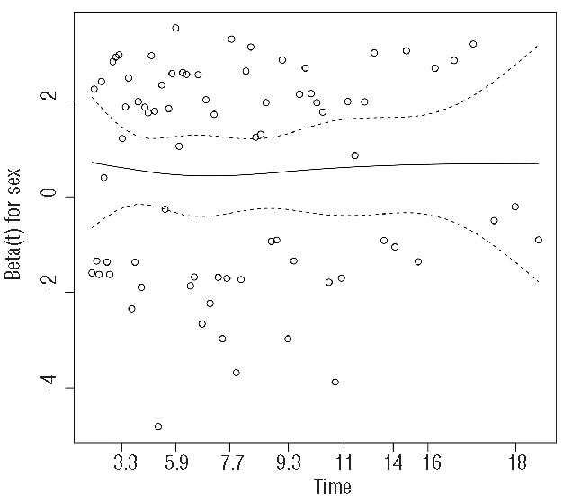
Plot of Schönfeld residuals against time in a Cox regression model evaluating the impact of sex on the overall survival of patients with CLL. The constant mean of residuals across time confirms that the proportional hazard assumption holds for this covariate. This plot was performed using R (version 3.0.1).

Figure 5.

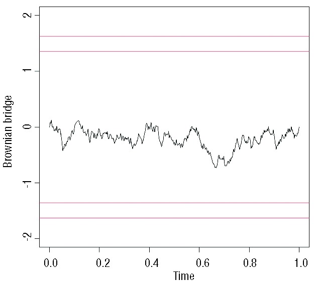
Brownian bridge depicting the constant effect of age on the relative survival of patients with CLL, thus validating the results observed in Figure 3. The proportional hazard assumption is met when the curve never crosses the horizontal lines up and above it (as in the example). This plot was performed using R (version 3.0.1).

Imagine now that one or more of your covariates violates the PH assumption. What can you do¿ Throw your results in the waste bin¿ Well, there are several ways of solving this problem in SPSS.

1. Introduce all covariates that meet the PH assumption in the model and leave out the covariate that does not meet the assumption. Alternatively, this covariate could be evaluated as a “stratum”. If the reader chooses to do it this way, SPSS will run two different regression models and give back a single result. Unfortunately, this result will not include any information regarding the “significance” of the stratum.

2. Include the covariate that does not meet the PH assumption in the model as time-dependent, which should be defined as “covariate+T_”. Please note the difference with the prior definition, the covariate is added and not multiplied, and no logarithmic transformation is required. Using this method, we would get information about the significance of the original time-fixed covariate through its time-dependent transformation.

3. Evaluate the interaction between the covariate that violates the PH assumption and the others by multiplying them (>a*b>). By doing this, you could generate new “combined” covariates that could meet the assumption and even have a higher statistical significance than both covariates separately.

Finally, we would like to end this section by emphasizing that the Cox proportional hazard regression model is just that, a model. It serves its purpose very well, which is to simultaneously explore the effects of several covariates on survival, but always under a proportional hazards assumption. Since all statistical packages offer the option of plotting ‘fitted’ data, some researchers elect to plot ‘fitted’ rather than ‘actual’ data because survival curves look nicer, usually more proportional than they actually are (not surprisingly!!). Please do not make that mistake! Fitted data should never be presented in a paper and, if for some reason you elect to do so, make sure the actual data are plotted too!

Competing risk regression models

As shown above, KM and Cox regression methods are appropriate when evaluating survival, but less so when we are interested in other end points that express competing events. For instance, in a recent paper, we were interested in evaluating the cumulative incidence of Richter’s transformation in our cohort of patients with CLL. For this analysis, we had to consider as competing events all deaths that occurred in patients without Richter’s transformation.⁴³ After evaluating each covariate separately using Gray’s test and plotting their cumulative incidence (not the complement of the KM curve), we then proceeded to perform a multivariate analysis.

Regression modeling in the context of competing events has been extensively reviewed over the last decade. Both non-parametric and regression methods exist, of which two are frequently used: the cause-specific relative hazard method of Kalbfleisch and Prentice,⁴⁴ and the subdistribution relative hazard method of Fine and Gray.⁴⁵ The latter method is our favorite and is, indeed, the method we applied in our previous example, where we found that both NOTCH1 mutations and IGHV mutational status were independent predictors of Richter’s transformation in our cohort.⁴³ A second paper published by Scrucca et al. explains how to implement the Fine and Gray method using R,⁴⁶ but this method is also included in Stata (Table 1). These methods depend upon the PH assumption which, in this particular situation, is slightly more time-consuming to check, but that can be easily done following Scrucca’s guidelines.⁴⁶ More recently, two alternative methods have been proposed, one by Klein and Andersen⁴⁷ which is, perhaps, a bit too complicated, and the so-called “mixture” model. This last method was initially proposed by Larson and Dinse⁴⁸ and has been extensively developed and evaluated by Lau et al.^49,50 The advantages of the “mixture” model are that it does not rely on the PH assumption and that, by being parametric, it tends to have a higher statistical power that semi- or non-parametric methods. This model requires some programming within SAS (NLMIXED procedure), but we have achieved nearly identical results in R (cmprsk package) simply by coding “failures” and “censors” in a slightly different way (Table 3).

Table 3.

Fine and Gray method versus parametric mixture model. Effect of history of injection drug use on the proportion and timing of incident HIV, treatment use, and incidence of AIDS or death (Women’s Interagency HIV Study, 1995–2005, United States). For the purpose of this comparative analysis, we have used the database provided by Lau et al.⁴⁰ The Fine and Gray method results were obtained using the R cmprsk package by modifying the failcode (fc) and cencode (cc) as follows: *fc=2, cc=0; **fc=2, cc=1; ***fc=1, cc=0; ****fc=1, cc=2.

Multiple imputation

As already stated, Cox models are very popular because they allow investigators to quantify the effects of a number of prognostic factors (covariates) while adjusting for imbalances that may be present in our patient cohort. Unfortunately, missing data are a common occurrence for most medical studies, and the fraction of patients with missing results could be relatively large in some of these studies. Moreover, it may happen that you have 15% missing results for covariate A, 15% missing results for covariate B, 20% missing results for covariate C, and 20% for covariate D. If all four covariates have a significant impact on survival by univariate analysis and you wish to fit a Cox proportional hazard regression model, any statistical software (SPSS, Stata or R) will only use those patients who have results for all four covariates, which could be only 40–50% of your patient cohort. As such, the more covariates you evaluate, the smaller the population and, therefore, it becomes progressively difficult to draw meaningful conclusions from your study. Consequently, omission of participants with missing values (also called complete case analysis) can have a big impact on the statistical power of your analysis and may lead to inadequate conclusions.^51–53

There are several methods for dealing with missing data: multiple imputation, maximum likelihood, fully Bayesian, weighted estimated equations, etc, but in this review we will only discuss multiple imputation. This method is becoming very popular and involves creating multiple complete data sets by filling in values for the missing data and analyzing these as if they were complete data sets. Then, all filled-in datasets are combined into one result by averaging over the filled-in datasets. We would like to emphasize that the purpose of multiple imputation is not to ‘create’ or ‘make up’ data but, on the contrary, to preserve real, observed data. We have evaluated three different R packages available for that purpose: Hmisc, mi and Amelia, of which Amelia (also known as Amelia II) is our favorite, because it is fast and relatively easy to use.⁵⁴ Moreover, for those who dislike the R software environment, this package incorporates AmeliaView, a graphical user interface that allows the user to set options and run Amelia without any prior knowledge of the R programming language. The newer versions of Stata also include some different methods for performing multiple imputation, but we have no experience with them.

Multiple imputation has, nevertheless, several drawbacks. One is that it produces different results every time you use it, since the imputed values are random draws rather than deterministic quantities. A second downside is that there are many different ways to do multiple imputation, which could easily lead to uncertainty and confusion. In a recent article, a group of researchers used multiple imputation to handle missing data and found (shockingly!) that cholesterol levels were not related to cardiovascular risk.⁵⁵ When asked about this by Prof. Peto, a revered statistician,⁵⁶ the authors performed a complete case analysis and found a clear association between cholesterol and cardiovascular risk, which was subsequently confirmed when the multiple imputation procedure was revised.⁵⁷ It is thus important to be aware of the problems that can occur with multiple imputation, which is why there is still much controversy around the issue and many statisticians question its basic value as a statistical tool.^58,59

Finally, we would not want to suggest that researchers could put less effort into collecting as many data as possible, or that multiple imputation could be a substitute for a carefully designed study or trial,⁶⁰ or that imputed results could be used to plot a survival curve. As stated above, survival curves should only plot actual data, never ‘imputed’ nor ‘modeled’ data.

However, every researcher faces the problem of missing values, irrespective of these efforts. To ‘provide’ data according to the strict methodology of multiple imputation seems a better alternative than to give up valuable observed data. Unfortunately, multiple imputation requires modeling the distribution of each variable with missing values in terms of the observed data, and the validity of results depends on such modeling being done adequately. Consequently, multiple imputation should not be regarded as a routine technique to be applied “at the push of a button”.⁵⁹ Indeed, whenever possible, specialist statistical help should be sought and obtained. Multiple imputation should be handled with care!

Conclusions

We would like to end our review with the following self-evaluation. When performing a survival analysis ask yourself the following questions.

1. Am I studying survival, or any other end point¿ Are there any competing events¿ Are all censored patients at risk of having the event in the future¿ If the answer to this last question is “no”, then you should consider calculating cumulative incidence and not KM curves.

2. Are all my covariates known at time zero¿ If not, consider changing the moment when you set the clock, or using time-dependent covariates, or even the Mantel-Byar test or a landmark analysis.

3. Can we attribute a significant proportion of the observed mortality to natural causes and not only to the disease of interest¿ If the answer is “yes”, consider estimating the relative survival adjusting your results according to your own national mortality tables.

4. Have I checked the proportional hazard assumption in my Cox regression model¿ If not, now you know how to do it!

We hope we have achieved our goal, which was to provide some basic concepts of survival analysis and also made some specific recommendations about how and when to perform each particular method. All the examples provided were computed using SPSS, Stata and R, because these are the statistical packages we like best. SPSS and Stata are available in many institutions worldwide, but they are also expensive. In contrast, R is available for free, so there is virtually no excuse for not doing the statistical method or test that is appropriate for each specific situation.

References

- 1.Abrisqueta P, Pereira A, Rozman C, Aymerich M, Giné E, Moreno C, et al. Improving survival in patients with chronic lymphocytic leukemia (1980–2008): the Hospital Clinic of Barcelona experience. Blood. 2009;114(10):2044–50. [DOI] [PubMed] [Google Scholar]
- 2.Lausen B, Schumacher M. Maximally selected rank statistics. Biometrics. 1992;48(1):73–85. [Google Scholar]
- 3.Kaplan EL, Meier P. Nonparametric estimation from incomplete observations. J Am Stat Assoc. 1958;53(282):457–81. [Google Scholar]
- 4.Klein JP, Rizzo JD, Zhang MJ, Keiding N. Statistical methods for the analysis and presentation of the results of bone marrow transplants. Part 2: Regression modeling. Bone Marrow Transplant. 2001;28(10):1001–11. [DOI] [PubMed] [Google Scholar]
- 5.Iacobelli S. on behalf of the EBMT Statistical Committee. Suggestions on the use of statistical methodologies in studies of the European Group for Blood and Marrow Transplantation. Bone Marrow Transplant. 2013;48(Suppl 1):S1–S37. [DOI] [PubMed] [Google Scholar]
- 6.Klein JP, Rizzo JD, Zhang MJ, Keiding N. Statistical methods for the analysis and presentation of the results of bone marrow transplants. Part I: unadjusted analysis. Bone Marrow Transplant. 2001;28(11):909–15. [DOI] [PubMed] [Google Scholar]
- 7.Weinberg JB, Volkheimer AD, Chen Y, Beasley BE, Jiang N, Lanasa MC, et al. Clinical and molecular predictors of disease severity and survival in chronic lymphocytic leukemia. Am J Hematol. 2007;82(12):1063–70. [DOI] [PubMed] [Google Scholar]
- 8.Tschumper RC, Geyer SM, Campbell ME, Kay NE, Shanafelt TD, Zent CS, et al. Immunoglobulin diversity gene usage predicts unfavorable outcome in a subset of chronic lymphocytic leukemia patients. J Clin Invest. 2008;118(1):306–15. [DOI] [PMC free article] [PubMed] [Google Scholar]
- 9.Shanafelt TD, Kay NE, Rabe KG, Call TG, Zent CS, Maddocks K, et al. Natural history of individuals with clinically recognized monoclonal B-cell lymphocytosis compared with patients with Rai 0 chronic lymphocytic leukemia. J Clin Oncol. 2009;27(24):3959–63. [DOI] [PMC free article] [PubMed] [Google Scholar]
- 10.Wierda WG, O’Brien S, Wang X, Faderl S, Ferrajoli A, Do KA, et al. Multivariable model for time to first treatment in patients with chronic lymphocytic leukemia. J Clin Oncol. 2011;29(31):4088–95. [DOI] [PMC free article] [PubMed] [Google Scholar]
- 11.Kim HT. Cumulative incidence in competing risks data and competing risks regression analysis. Clin Cancer Res. 2007;13(2):559–65. [DOI] [PubMed] [Google Scholar]
- 12.Gray R. A class of k-sample tests for comparing the cumulative incidence of a competing risk. Ann Stat. 1988;16(3):1141–54. [Google Scholar]
- 13.Scrucca L, Santucci A, Aversa F. Competing analysis using R: an easy guide for clinicians. Bone Marrow Transplant 2007;40(4):381–7. [DOI] [PubMed] [Google Scholar]
- 14.Timp JF, Braekkan SK, Versteeg HH, Cannegieter SC. Epidemiology of cancer-associated venous thrombosis. Blood. 2013;122(10):1712–23. [DOI] [PubMed] [Google Scholar]
- 15.Lee AY, Levine MN, Baker RI, Bowden C, Kakkar AK, Prins M, et al. Low-molecular-weight heparin versus a coumarin for the prevention of recurrent venous thromboembolism in patients with cancer. N Engl J Med. 2003;349(2):146–53. [DOI] [PubMed] [Google Scholar]
- 16.Ay C, Simanek R, Vormittag R, Dunkler D, Alguel G, Koder S, et al. High plasma levels of soluble P-selectin are predictive of venous thromboembolism in cancer patients: results from the Vienna Cancer and Thrombosis Study (CATS). Blood. 2008;112(7):2703–8. [DOI] [PubMed] [Google Scholar]
- 17.Campigotto F, Neuberg D, Zwicker JI. Biased estimation of thrombosis rates in cancer studies using the method of Kaplan and Meier. J Thromb Haemost. 2012;10(7):1449–51. [DOI] [PMC free article] [PubMed] [Google Scholar]
- 18.Agnelli G, George DJ, Kakkar AK, Fisher W, Lassen MR, Mismetti P, et al. Semuloparin for thromboprophylaxis in patients receiving chemotherapy for cancer. N Engl J Med. 2012;366(7):601–9. [DOI] [PubMed] [Google Scholar]
- 19.Anderson JR, Cain KC, Gelber RD. Analysis of survival by tumor response. J Clin Oncol. 1983;1(11):710–9. [DOI] [PubMed] [Google Scholar]
- 20.Anderson JR, Cain KC, Gelber RD. Analysis of survival by tumor response and other comparisons of time-to-event by outcome variables. J Clin Oncol. 2008;26(24):3913–5. [DOI] [PubMed] [Google Scholar]
- 21.Mantel N, Byar DP: evaluation of response-time data involving transient states: an illustration using heart-transplant data. J Am Stat Assoc. 1974;69(345):81–6. [Google Scholar]
- 22.Cantor A. A test of the association of a time-dependent state variable to survival. Comput Methods Programs Biomed. 1995;46(2):101–5. [DOI] [PubMed] [Google Scholar]
- 23.Cornelissen JJ, van Putten WL, Verdonck LF, Theobald M, Jacky E, Daenen SM, et al. Results of a HOVON/SAKK donor versus no-donor analysis of myeloablative HLA-identical sibling stem cell transplantation in first remission acute myeloid leukemia in young and middle-aged adults: benefits for whom¿ Blood. 2007;109(9):3658–66. [DOI] [PubMed] [Google Scholar]
- 24.Koreth J, Schlenk R, Kopecky KJ, Honda S, Sierra J, Djulbegovic BJ, et al. Allogeneic stem cell transplantation for acute myeloid leukemia in first complete remission: systematic review and meta-analysis of prospective clinical trials. JAMA. 2009;301(22):2349–61. [DOI] [PMC free article] [PubMed] [Google Scholar]
- 25.Burnett AK. Treatment of acute myeloid leukemia: are we making progress¿ Hematology (Am Soc Hematol Educ Program). 2012;2012:1–6. [DOI] [PubMed] [Google Scholar]
- 26.Dafni U. Landmark analysis at the 25-year landmark point. Circ Cardiovasc Qual Outcomes. 2011;4(3):363–71. [DOI] [PubMed] [Google Scholar]
- 27.Shanafelt TD, Witzig TE, Fink SR, Jenkins RB, Paternoster SF, Smoley SA, et al. Prospective evaluation of clonal evolution during long-term follow-up of patients with untreated early-stage chronic lymphocytic leukemia. J Clin Oncol. 2006;24(28):4634–41. [DOI] [PubMed] [Google Scholar]
- 28.Siegel R, Ma J, Zou Z, Jemal A. Cancer statistics, 2014. CA Cancer J Clin. 2014;64(1):9–29. [DOI] [PubMed] [Google Scholar]
- 29.Howlader N, Noone AM, Krapcho M, Garshell J, Miller D, Altekruse SF, et al. (editors). SEER Cancer Statistics Review, 1975–2009 (Vintage 2009 Populations), based on November 2011 SEER data submission, posted to the SEER web site, 2012. Available from: http://seer.cancer.gov/csr/1975_2009_pops09/ Accessed: March 10,2013.
- 30.Tsimberidou AM, Wen S, McLaughlin P, O’Brien S, Wierda WG, Lerner S, et al. Other malignancies in chronic lymphocytic leukemia/small lymphocytic lymphoma. J Clin Oncol. 2009;27(6):904–10. [DOI] [PMC free article] [PubMed] [Google Scholar]
- 31.Morton LM, Curtis RE, Linet MS, Bluhm EC, Tucker MA, Caporaso N, et al. Second malignancy risks after non-Hodgkin’s lymphoma and chronic lymphocytic leukemia: differences by lymphoma subtype. J Clin Oncol. 2010;28(33):4935–44. [DOI] [PMC free article] [PubMed] [Google Scholar]
- 32.Dickman PW, Adami HO. Interpreting trends in cancer patient survival. J Intern Med. 2006;260(2):103–17. [DOI] [PubMed] [Google Scholar]
- 33.Ederer F, Axtell LM, Cutler SJ. The relative survival rate. Natl Cancer Inst Monograph. 1961;6:101–27. [PubMed] [Google Scholar]
- 34.Talbäck M, Dickman PW. Estimating expected survival probabilities for relative survival analysis – Exploring the impact of including cancer patient mortality in the calculations. Eur J Cancer. 2011;47(17):2626–32. [DOI] [PubMed] [Google Scholar]
- 35.Dickman PW, Sloggett A, Hills M, Hakulinen T. Regression models for relative survival. Stat Med. 2004;23(1):51–64. [DOI] [PubMed] [Google Scholar]
- 36.Pohar M, Stare J. Relative survival analysis in R. Comput Methods Programs Biomed. 2006;81(3):272–8. [DOI] [PubMed] [Google Scholar]
- 37.Pohar M, Stare J. Making relative survival analysis relatively easy. Comput Biol Med. 2007;37(12):1741–9. [DOI] [PubMed] [Google Scholar]
- 38.Roche L, Danieli C, Belot A, Grosclaude P, Bouvier AM, Velten M, et al. Cancer net survival on registry data: use of the new unbiased Pohar-Perme estimator and magnitude of the bias with the classical methods. Int J Cancer. 2013;132(10):2359–69. [DOI] [PubMed] [Google Scholar]
- 39.Dickman PW, Lambert PC, Coviello E, Rutherford MJ. Estimating net survival in population-based cancer studies. Int J Cancer. 2013;133(2):519–21. [DOI] [PubMed] [Google Scholar]
- 40.Cox DR. Regression models and life-tables. J R Stat Soc B. 1972;34(2):187–220. [Google Scholar]
- 41.López C, Delgado J, Costa D, Villamor N, Navarro A, Cazorla M, et al. Clonal evolution in chronic lymphocytic leukemia: analysis of correlations with IGHV mutational status, NOTCH1 mutations and clinical significance. Genes Chromosomes Cancer. 2013;52(10):920–7 [DOI] [PubMed] [Google Scholar]
- 42.Grambsch P, Therneau T. Proportional hazards tests and diagnostics based on weighted residuals. Biometrika. 1994;81(3):515–26. [Google Scholar]
- 43.Villamor N, Conde L, Martínez-Trillos A, Cazorla M, Navarro A, Beà S, et al. NOTCH1 mutations identify a genetic subgroup of chronic lymphocytic leukemia patients with high risk of transformation and poor outcome. Leukemia. 2013;27(5):1100–6 [DOI] [PubMed] [Google Scholar]
- 44.Prentice RL, Kalbfleisch JD, Peterson AV, Jr, Flournoy N, Farewell VT, Breslow NE. The analysis of failure times in the presence of competing risks. Biometrics. 1978;34(4):541–54. [PubMed] [Google Scholar]
- 45.Fine JP, Gray RJ. A proportional hazards model for the subdistribution of a competing risk. J Am Stat Assoc. 1999;94(446):496–509. [Google Scholar]
- 46.Scrucca L, Santucci A, Aversa F. Regression modeling of competing risk using R: an in depth guide for clinicians. Bone Marrow Transplant. 2010;45(9):1388–95. [DOI] [PubMed] [Google Scholar]
- 47.Klein JP, Andersen PK. Regression modeling of competing risks data based on pseudovalues of the cumulative incidence function. Biometrics. 2005;61(1):223–9. [DOI] [PubMed] [Google Scholar]
- 48.Larson MG, Dinse GE. Mixture models for the regression analysis of competing data. J R Stat Soc C. 1985;34(3):201–11. [Google Scholar]
- 49.Lau B, Cole SR, Gange SJ. Competing risk regression models for epidemiologic data. Am J Epidemiol. 2009;170(2):244–56. [DOI] [PMC free article] [PubMed] [Google Scholar]
- 50.Lau B, Cole SR, Gange SJ. Parametric mixture models to evaluate and summarize hazard ratios in the presence of competing risks with time-dependent hazards and delayed entry. Stat Med. 2011;30(6):654–65. [DOI] [PMC free article] [PubMed] [Google Scholar]
- 51.Ibrahim JG, Chu H, Chen MH. Missing data in clinical studies: issues and methods. J Clin Oncol. 2012;30(26):3297–303. [DOI] [PMC free article] [PubMed] [Google Scholar]
- 52.Groenwold RH, Donders AR, Roes KC, Harrell FE, Jr, Moons KG. Dealing with missing outcome data in randomized trials and observational studies. Am J Epidemiol. 2012;175(3):210–7. [DOI] [PubMed] [Google Scholar]
- 53.Janssen KJ, Donders AR, Harrell FE, Jr, Vergouwe Y, Chen Q, Grobbee DE, et al. Missing covariate data in medical research: to impute is better than to ignore. J Clin Epidemiol. 2010;63(7):721–7. [DOI] [PubMed] [Google Scholar]
- 54.Honaker J, King G, Blackwell M. Amelia II: a program for missing data. J Stat Software. 2011;45(7):1–47. [Google Scholar]
- 55.Hippisley-Cox J, Coupland C, Vinogradova Y, Robson J, May M, Brindle P. Derivation and validation of QRISK, a new cardiovascular disease risk score for the United Kingdom: prospective open cohort study. BMJ. 2007;335(7611):136–41. [DOI] [PMC free article] [PubMed] [Google Scholar]
- 56.Peto R. Doubts about QRISK score: total/HDL cholesterol should be important [electronic response to Hippisley-Cox J, et al]. BMJ. 2007, July 13th. Available from: http://www.bmj.com/rapid-response/2011/11/01/doubts-about-qrisk-score-total-hdl-cholesterol-should-be-important.
- 57.Hippisley-Cox J, Coupland C, Vinogradova Y, Robson J, May M, Brindle P. QRISK— authors’ response [electronic response]. BMJ. 2007. August 7th. Available from: http://www.bmj.com/rapid-response/2011/11/01/qrisk-authors-response.
- 58.Allison PD. Multiple imputation for missing data: a cautionary tale. Sociological Methods & Res. 2000; 28(3):301–9. [Google Scholar]
- 59.Sterne JA, White IR, Carlin JB, Spratt M, Royston P, Kenward MG, et al. Multiple imputation for missing data in epidemiological and clinical research: potential and pitfalls. BMJ. 2009;338:b2393. [DOI] [PMC free article] [PubMed] [Google Scholar]
- 60.Liu M, Wei L, Zhang J. Review of guidelines and literature for handling missing data in longitudinal clinical trials with a case study. Pharm Stat. 2006;5(1):7–18. [DOI] [PubMed] [Google Scholar]