An intelligent approach for variable size segmentation of non-stationary signals

Abstract

In numerous signal processing applications, non-stationary signals should be segmented to piece-wise stationary epochs before being further analyzed. In this article, an enhanced segmentation method based on fractal dimension (FD) and evolutionary algorithms (EAs) for non-stationary signals, such as electroencephalogram (EEG), magnetoencephalogram (MEG) and electromyogram (EMG), is proposed. In the proposed approach, discrete wavelet transform (DWT) decomposes the signal into orthonormal time series with different frequency bands. Then, the FD of the decomposed signal is calculated within two sliding windows. The accuracy of the segmentation method depends on these parameters of FD. In this study, four EAs are used to increase the accuracy of segmentation method and choose acceptable parameters of the FD. These include particle swarm optimization (PSO), new PSO (NPSO), PSO with mutation, and bee colony optimization (BCO). The suggested methods are compared with other most popular approaches (improved nonlinear energy operator (INLEO), wavelet generalized likelihood ratio (WGLR), and Varri’s method) using synthetic signals, real EEG data, and the difference in the received photons of galactic objects. The results demonstrate the absolute superiority of the suggested approach.

Introduction

Generally speaking, signals can be categorized in two main types, namely, deterministic signals and non-deterministic signals. A non-deterministic signal is the one with varying statistical properties and can be considered random in analysis. Most of physiological signals, such as electroencephalogram (EEG) and electrocardiogram (ECG) signals, are of this type. Attending at the process, random signals can be divided into two main classes: stationary and non-stationary signals. Unlike in non-stationary signals, the statistical properties, such as mean and variance, do not change in stationary signals.

Since processing stationary signals is much easier and less complicated than non-stationary ones, the signal is often broken into segments within which the signals can be considered stationary. In this way, each part can be analyzed or processed separately [1–3]. This approach is taken in a number of signal processing applications such as tracking the changes in brightness of galactic objects [1] and EEG signal processing [2].

Generally, there are two types of segmentations for non-stationary signals. In the first type, the signal is segmented into equal parts. This process is called fixed-size segmentation. Although computing fixed-size segmentations is simple, it does not have sufficient accuracy [4]. In the second technique used for non-stationary signals, which is called adaptive segmentation, the signals are automatically segmented into variable parts of different statistical properties [2].

The generalized likelihood ratio (GLR) method has been suggested to obtain the boundaries of signal segments by using two windows that slide along the signal. The signal within each window of this algorithm is modeled by an auto-regressive model (AR). In the case where the windows are placed in a segment, their statistical properties do not differ. In other words, the AR coefficients remain roughly constant and equal. On the other hand, if the sliding windows fall in dissimilar segments, the AR coefficients change and the boundaries are detected [5]. Lv et al. have suggested using wavelet transform to decrease the number of false segments and reduce the computation load [6]. This method has been named wavelet GLR (WGLR) [6].

Agarval and Gotman proposed the nonlinear energy operator (NLEO) in order to segment the electroencephalographic signals using the following equation [7]:

$${\psi }_d[x(n)]=x^2(n)-x(n-1)x(n+1)$$ (1)

If x(n) is a sinusoidal wave, then, ψ[x(n)] will be defined as follows:

$$Q(n)=\psi [A\cos ({\omega }_{0}n+\theta )]=A^2{\sin }^2{\omega }_0$$ (2)

when ω₀ is much smaller than the sampling frequency, then $Q(n)=A^2{\omega }_0^2$. In fact, any change in amplitude (A) and/or frequency (ω₀) can be discovered in Q(n). In the case of a multi-component signal, Hassanpour and Shahiri [8] demonstrated that the linear operation creates cross-terms, something that defeats the purpose of the NLEO method in properly segmenting the signal. In order to reduce the effects of cross-terms in the NLEO method, using the wavelet transform has been proposed [8]. This new method is known as improved nonlinear energy operator (INLEO).

A novel approach for non-stationary signal segmentation in general, and real EEG signal in particular, based on standard deviation, integral operation, discrete wavelet transform (DWT), and variable threshold has been proposed [9]. In this paper, it was illustrated that the standard deviation can indicate changes in the amplitude and/or frequency [9]. In order to take away the impact of shifting and smooth the signal, the integral operation was utilized as a pre-processing step although the performance of the method is still relevant on the noise components.

Several powerful image segmentation methods using hidden Markov model (HMM) [10], triplet Markov chains (TMC) [11], and pairwise Markov model (PMM) [11] have been proposed by Lanchantin et al. [11]. These methods have been validated by different experiments, some of which are related to semi-supervised and unsupervised image segmentation. It should be mentioned that these approaches can be used and discussed in non-stationary and stationary signal segmentation approaches too.

Inasmuch as real time series are usually nonlinear and to extract important information from the measured signals, it is significant to utilize a pre-processing step, such as a wavelet transform (WT), to reduce the effect of noise [12]. DWT represents the signal variation in frequency with respect to time.

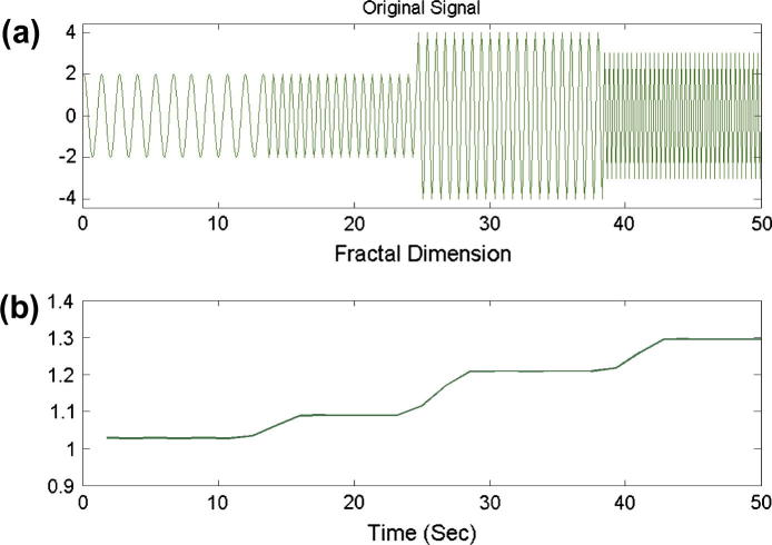
After decomposing the signal, fractal dimension (FD) is employed as a relevant tool to detect the transients in a signal [13]. FD can be used as a feature for adaptive signal segmentation because FD can indicate changes not only in amplitude but also in frequency. Fig. 1 shows when the amplitude and/or frequency of a signal are changed, the FD changes. The original signal consists of four segments. The first and second segments have the same amplitude. The frequency of the first part is, however, dissimilar from that of the second part. The amplitude of the third segment is different from that of the second segment. The fourth segment is different from the third one in terms of both amplitude and frequency. This signal illustrates that if two adjacent epochs in a time series have different frequencies and/or amplitudes, the FD will change.

Fig. 1.

Variation in FD when amplitude or frequency changes.

Two key parameters for FD-based detection of transients in the signals are determined experimentally. These are the window length and the overlapping percentage of successive windows. Small windows might not be fully capable of clarifying long-term statistics suitably whereas long windows may overlook small block variations. The overlapping percentage of the successive windows influences both the correctness of the segmentation results and the computational load.

To achieve accurate segmentations, here we investigate the use of particle swarm optimization (PSO), new PSO (NPSO) and PSO with mutation, and bee colony optimization (BCO) to estimate the aforementioned parameters. These algorithms are fast search techniques that can obtain precise or locally optimal estimations in the desired search space.

The other sections of this paper are organized as follows. In ‘Fractal dimension’ Katz’s method to calculate the FD has been explained in brief. ‘Evolutionary algorithms’ introduces four methods in EAs, including PSO, NPSO, the proposed PSO with mutation, and BCO. ‘Proposed adaptive signal segmentation’ represents the proposed methods in four steps. The description of three types of data (synthetic data, real EEG signals, and real photon emission data) is included in ‘Simulation data and results’. Subsequently, the performance of the proposed methods is compared with the outputs of some of the existing methods including, three powerful evolutionary approaches based on the FD, WGLR, INLEO, and Varri’s methods. The last section concludes the paper.

The hybrid approach

Fractal dimension

The FD of a signal can be a powerful tool for transient detection. FD is widely used for image segmentation, analysis of audio signals, and analysis of biomedical signals such as EEG and ECG [14,15]. Also, FD is a useful method to indicate variations in both amplitude and frequency of a signal.

There are several specific algorithms to compute the FD, such as Katz’s, Higuchi’s, and Petrosian’s. All of these algorithms have advantages and disadvantages, and the most appropriate one depends on the application [15].

Katz’s algorithm is slightly slower than Petrosian’s. In Katz’s algorithm, unlike in Petrosian’s, no pre-processing is required to create a binary sequence. This algorithm can be implemented directly on the analyzed signal. In this method, the dimension of FD of a signal can be defined as follows [15]:

$$\text{FD}=\frac{\log (L)}{\log (d)}$$ (3)

where L depicts length of the time series or the total distance between consecutive points and d illustrates the maximum distance between the first data of time series and the data that have maximum distance from it. Mathematically, d can be defined by the following equation:

$$d=\max (\text{distance}(x_1\text{,}{x}_i))$$ (4)

where x_i is the ith data point that has maximum distance from the first data point of the time sequence at time point l [15].

Evolutionary algorithms

Particle swarm optimization

PSO is a fast, powerful evolutionary algorithm, inspired by nature, initially proposed by Kennedy and Eberhart in 1995 [16]. The social behavior of animals such as birds and fish at what time they are together was the inspiration source for this method [16]. PSO, such as other evolutionary algorithms, initiates with a random matrix as an initial population. Unlike genetic algorithms (GAs), standard PSO does not have evolutionary operators such as breeding and mutation. Each member of the population is called a particle. In this method, a certain number of particles formed at random make the primary values. There are two parameters for each particle: position and velocity, which are defined, respectively, by a space vector and a velocity vector. These particles shape a pattern in an n-dimensional space and move to the desired value. The most optimum position of each particle in the past and the best position among all particles are stored separately. Based on the experience from the prior moves, the particles decide how to move in the next step. In each iteration, all particles in the n-dimensional problem space go to an optimum point and, in every iteration, the position and velocity of each particle can be amended as follows

$$v_i(t+1)={\mathit{wv}}_i(t)+C_1{r}_1(p_{{\mathit{best}}_i}(t)-x_i(t))+C_2{r}_2(g_{{\mathit{best}}_i}(t)-x_i(t))$$ (5)

$$x_i(t+1)=x_i(t)+v_i(t+1)$$ (6)

where n stands for the dimension (1 ⩽ n ⩽ N), C₁ and C₂ are positive constants, generally considered 2.0. r₁ and r₂ are random numbers uniformly between 0 and 1; w is an initial weight that can be defined as a constant number [17].

Eq. (6) indicates that the velocity vector of each particle is updated (v_i(t + 1)) and the latest and previous values of the vector position (x_i(t)) make the new position vector (x_i(t + 1)). As a matter of fact, the updated velocity vector influences both the local and global values. The best global solution (g_best) and the best solution of the particle (p_best) stand for the best response of the entire particles and the best answer of the local positions, respectively.

Since PSO stays in local minima of fitness function, we use two techniques, namely, NPSO and PSO with mutation. In each iteration, as was mentioned in PSO, the global best particle and the local best particle are computed. The NPSO strategy uses the global best particle and local “worst” particle, the particle with the worst fitness value until current execution time [17]. It can be defined as follows:

$$v_i(t+1)={\mathit{wv}}_i(t)+C_1{r}_1(p_{{\mathit{worst}}_i}(t)-x_i(t))+C_2{r}_2(g_{{\mathit{best}}_i}(t)-x_i(t))$$ (7)

Mutation is defined as a physiologically-inspired disturbance to the system. It is frequently employed to branch away from potential local minima. In this paper, we propose to use mutation in PSO to keep away from local minima. To model this technique, in the beginning, two constants m₁ and m₂ are defined as thresholds. For each bit of x_i(t) a random number between 0 and 1 is generated. Then, if the random number for this bit is larger than a pre-defined “m₁”, that bit is flipped. Similarly, after creating a random number for each bit of v_i(t), if the random number is greater than a pre-defined “m₂”, that bit is flipped.

Bee colony optimization

The BCO is a novel population-based optimization algorithm which was proposed in 2005 by Karaboga [18]. Properties such as searching manner, reminding information, learning new information, and exchanging information cause the BCO to be one of the best algorithms in artificial intelligence [19].

Today, BCO and artificial bee colony (ABC) algorithms have remarkable applications, such as optimizing the traveling salesman problem (TSP) and the weights of multilayered perceptrons (MLP), controlling chart pattern recognition, designing digital IIR filters, and data clustering [18–20].

BCO is inspired and developed based on inspecting the attitudes of the real bees on discovering nectar and sharing the food sources information with the other bees in the hive. Generally, the agents in BCO are divided into the employed bees, the scout bees and the onlooker bees. The employed bees stay on a food sources and memorize the vicinity of the sources. The onlooker bees take the information of food sources from the employed bees in the hive and select one of the food sources to gather the nectar. The 3rd type of bees, who are called scouts, are responsible for finding new food, nectars, and sources [18–20].

The steps in BCO are inspired by the fact that, first, a colony of scout bees is sent to look for food promising flower patches. The movement of a scout is completely random from one patch to another. When scouts return to the hive, they give the attained information to other bees by going to a place called the “dance floor” and performing a dance that is known as the “waggle dance.” This dance declares three kinds of information including the direction in which the food can be found, destination distance from the hive (duration of the dance) and its quality rating (frequency of the dance). This attained information leads the other bees to find the flower patches accurately without guides or maps. After the dance, the scout bee goes back to the flower patch with a number of bees that were waiting inside the hive. The Pseudocode of the basic BCO is shown in Fig. 2 [18–20].

Fig. 2.

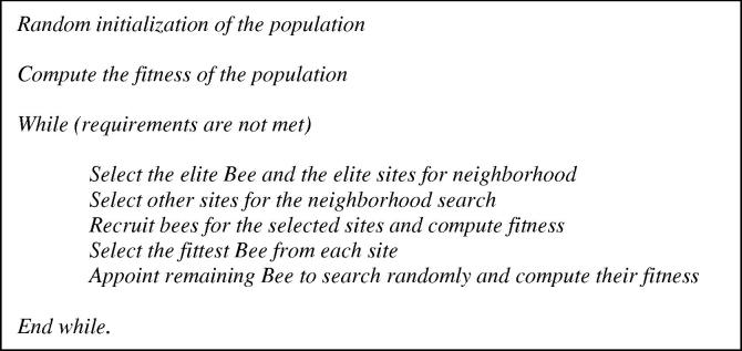
Pseudo code of the basic BCO.

The techniques described in ‘Evolutionary algorithms and Proposed adaptive signal segmentation’ are utilized in developing a new adaptive segmentation algorithm as explained in the following sections.

Proposed adaptive signal segmentation

In this part the suggested approach is explained comprehensively in three steps as follows:

• 1.The original signal is firstly decomposed using Daubechies wavelet [21] of order 8. This decomposition can demonstrate the gradually changing features of the signal in the lower frequency bands. In addition, for real signals such as the EEG, DWT can also be used as a time–frequency filtering approach to remove the undesired artifacts such as EMG and ECG.
• 2.We proposed to employ the Higuchi’s FD and DWT for signal segmentation [21]. Although DWT could diminish the effect of the noise to a certain extent [17] the proposed signal segmentation approach was still dependent on the noise level. As mentioned before [15], the Katz’s FD is much more robust to the noise and quicker than Higuchi’s FD. Thus, in this study, we use the Katz’s FD to reveal amplitude and/or frequency changes. The FDs of the decomposed signal are computed using the previously described sliding windows. Variation in the FD is used to obtain the segment boundaries as follows:

$$G_t=|{\text{FD}}_{t+1}-{\text{FD}}_t|t=1\text{,}2\text{,}\dots \text{,}L-1$$ (8)

where t and L stand for the number of analyzed windows and the total number of analyzed windows, respectively.

As explained before, the two parameters that influence the accuracy of the delineation of signal boundaries are the length of the window and percentage of overlapping of the sliding window. If they are not selected properly, the segment boundaries may be inexact. GA and imperialist competitive algorithm (ICA) have been proposed to vary the length and overlapping percentage upto some acceptable amount. In this part, in order to increase the performance and speed of the GA and ICA, we employ four EAs including PSO, PSO with mutation, NPSO and BCO. Note that, generally, among the mentioned EAs, the best evolutionary algorithm with similar parameters in terms of minimum fitness value is BCO. Fitness function of the EAs over k shifts of the successive window is chosen as:

$$E_G=\frac{{\sum }_{t=0}^k|\mathit{ceil}(G_t-\mathit{mean}(G_t)){|}^2}{N}$$ (9)

where N depicts the number of samples in G and ceil stands for ceiling.

Determining a threshold is one of the most vital problems in signal segmentation. In numerous pieces of research, the mean value or sum of the mean value and standard deviation (or a similar offset value) is suggested as a threshold. In case the defined threshold is large, some segment boundaries may not be detected. In contrast, if the threshold is low, some idle points may be inaccurately detected as boundaries. In this article the mean value of G $(\bar{G})$ is defined as the threshold. When the local maximum is bigger than the threshold, the current time is selected as the segment boundary.

Simulation data and results

The existing and proposed methods were simulated using MATLAB R2009a from Math Works, Inc. The performance and efficiency of these methods were evaluated using a set of synthetic multi-component data, real EEG data and the difference in the received photons of galactic objects downloaded from NASA’s website (http://adsabs.harvard.edu/abs/1998ApJ...504..405S).

Simulated data

In order to create signals similar to actual recordings, we added Gaussian noise to original signals and after that evaluated the performance of the proposed method. In this paper, 50 synthetic multi-component signals were used. Their equation is as follows:

$$y(t)=x(t)+n(t)$$ (10)

where n(t) expresses white Gaussian noise and x(t) is produced by concatenating seven multi-component epochs. One of 50 signals contains seven epochs with duration between 5.5 and 8 s as follows:

• •Epoch 1: 2.5 cos(2πt) + 1.5 cos(4πt) + 1.5 cos(6πt),
• •Epoch 2: 1.5 cos(2πt) + 4 cos(11πt),
• •Epoch 3: 1.3 cos(πt) + 4.5 cos(7πt),
• •Epoch 4: 1.5 cos(πt) + 4.5 cos(2πt) + 1.8 cos(6πt),
• •Epoch 5: 2 cos(2πt) + 1.4 cos(6πt) + 8 cos(10πt),
• •Epoch 6: 0.5 cos(3πt) + 4.7 cos(8πt),
• •Epoch 7: 0.8 cos(3πt) + cos(5πt) + 3 cos(8πt).

In this paper we used n(t) as Gaussian noise with SNR = 5, 10, and 15 dBs.

Secondly, we used real EEG signals. The registration of electrical activity of the neurons in the brain is called EEG and it is an important tool in identifying and treating some neurological disorders such as epilepsy. In this paper, 40 EEG signals recorded from the scalp of ten patients were used. The length of signals and the sampling frequency were 30 s and 256 Hz, respectively.

The study of galactic objects is a key area of astronomy [1]. For instance, when a moving galactic object is moving in front of a star, there are changes in the brightness received from the star. By studying and analyzing this brightness, we can acquire important data such as the size and the orbit of the galactic objects. The rate of the photons’ arrival shows some major statistical changes. This could be because of the creation of a new source or because of an explosion or a sudden boost in the brightness of an existing source. Here, it is assumed that the sampling rate is two micro-seconds.

Fig. 3a depicts a signal giving information about the received number of photons. Fig. 3a can be mulled as a Poisson distribution. By calculating the difference in time of the signal in Fig. 4a, we could obtain a signal that is a representation of the number of input photons – in each time instant (Fig. 3b).

Fig. 3.

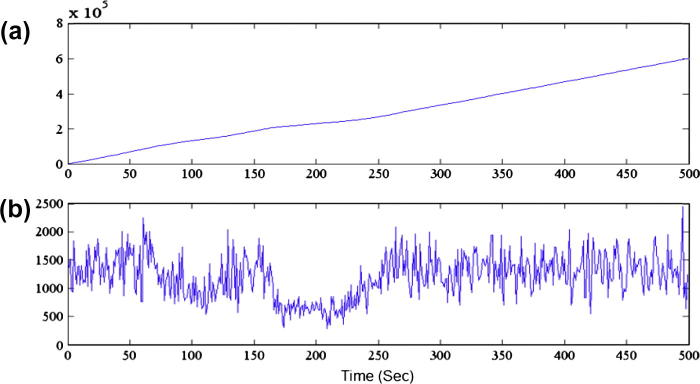
Real photon emission data; (a) the number of received photons as a function of time and (b) the difference between the received photons.

Fig. 4.

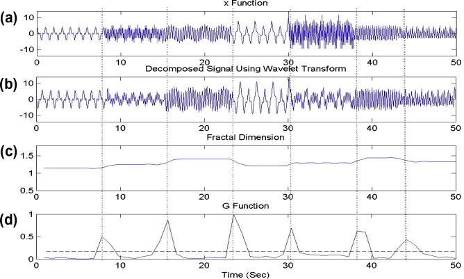
Results of applying the proposed technique with BCO to (a) original signal, (b) decomposed signal by one-level DWT, (c) output of FD, and (d) G function result. As it can be seen that the boundaries for all seven segments can be accurately detected.

Simulation results

The synthetic signal y(t) with SNR = 15 dB in Fig. 4a is firstly decomposed using one-level DWT. In this article, we employed DWT with Daubechies wavelet of order 8. This decomposed signal is depicted in Fig. 4b. As can be seen, the decomposed signal is considerably smoother than the original signal. Fig. 4c and d respectively show the FD of the decomposed signal and changes in the G function.

Usually, the window length and overlapping percentage of the sliding windows are the most important parameters for the conventional methods. In fact, adjusting these parameters empirically is the most important problem in those methods. To overcome this problem, we suggest using the EAs.

Choosing an adequate preliminary population and number of iterations is very significant in EAs. For lower values of these parameters, the speed of the proposed approach noticeably increases. On the other hand, for larger values of the chosen parameters the speed of the proposed methods drastically decreased. In all EAs, we must achieve the right balance for the parameters in the application. In a general manner, this trade-off is only made by trials and errors. In the proposed method, the parameters of PSO, NPSO, and PSO with mutation are: population size = 30; C1 = C2 = 2; Dimension = 2; Iteration = 50; w = 1; m₁ = 0.1; m₂ = 0.05 (for PSO with mutation). The next algorithm used in this paper is BCO. The parameters of this algorithm are defined as: population size = 30; Dimension = 2; Iteration = 50. In addition, length of the windows and the percentage of overlap for all these EAs are selected between 2% and 10% of the signal length. When the preliminary populations and number of iterations were increased, the efficiency of the suggested method was not significantly changed. Hence, for this application of the EAs, these populations and number of iterations were assumed to be correctly chosen.

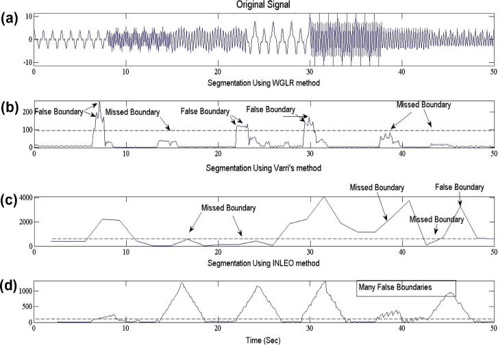
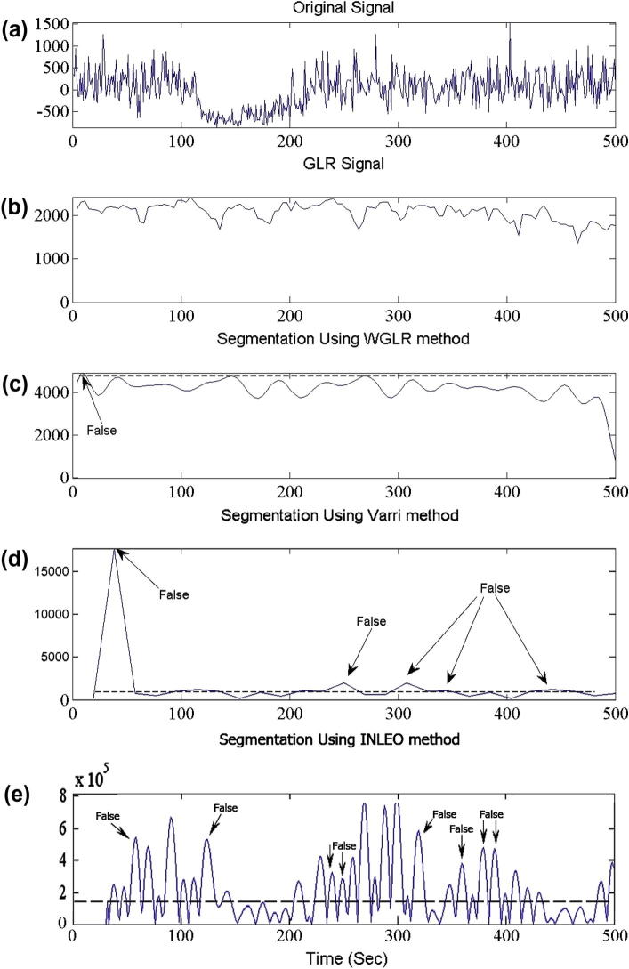
The signal in Fig. 4a is also segmented using three existing method, namely, WGLR [10], INLEO [8] and Varri’s [22] methods in Fig. 5. Although the INLEO method could indicate each six boundaries, this method had many false boundaries. The WGLR method found just three boundaries out of the six boundaries. Therefore, this method was unreliable to segment multi-component signals with noise. Finally, Varri’s method had several missed boundaries and false boundaries. In other words, this method had low performance too.

Fig. 5.

Results of applying the existing techniques; (a) original signal, (b) output of WGLR method, (c) output of Varri’s method, and (d) output of INLEO method.

To compare the convergence speed and accuracy of PSO, NPSO and PSO with mutation, the convergence characteristics of these algorithms for above-mentioned signal are illustrated in Fig. 6.

Fig. 6.

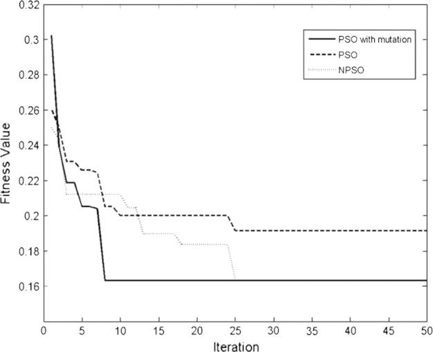
Comparison between the performances of PSO, NPSO, and PSO with mutation.

As it can be seen in Fig. 6, PSO with mutation converges to the global solution faster, while the other algorithms have trapped in the local optima. Fig. 7 represents the minimum fitness values of BCO particles and PSO with mutation versus iterations. The comparison results show that BCO reaches smaller values of G function.

Fig. 7.

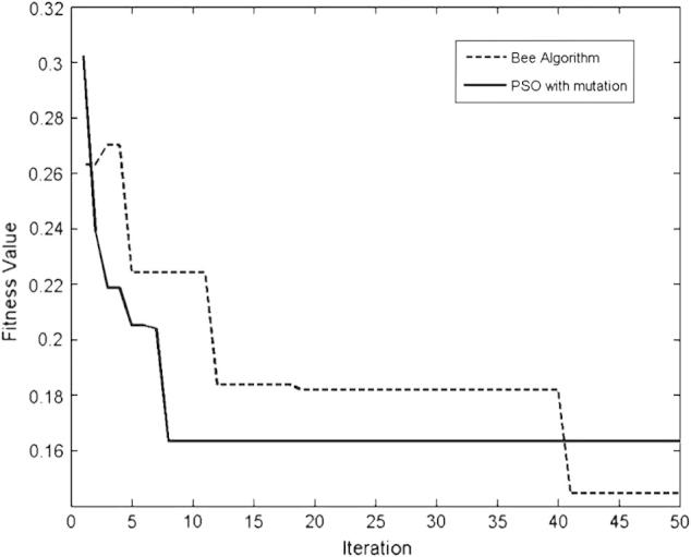
Comparison between the performances of PSO with mutation and BCO.

Three different metrics, including true positive (TP) false negative (FN) and false positive (FP) ratios are used to assess the performance and efficiency of the proposed and existing methods. These parameters defined as TP = (N_t/N), FN = (N_m/N), and FP = (N_f/N).

where N_t, N_m and N_f denote the number of true, missed and falsely detected boundaries respectively. N represents the actual number of signal boundaries.

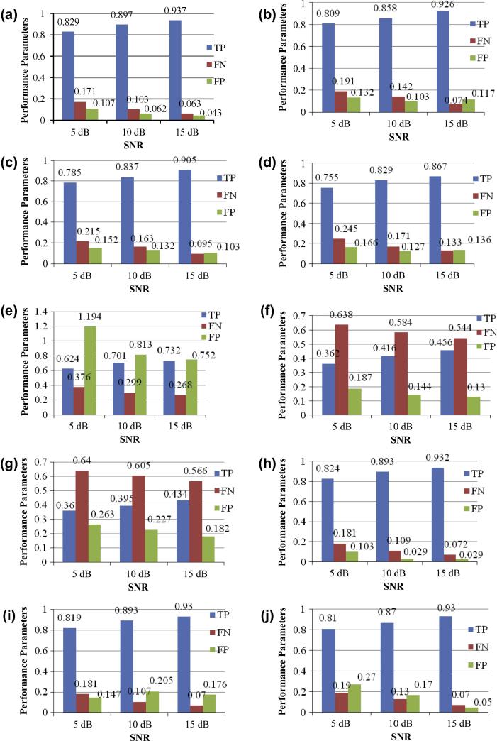
In Fig. 8 the results of the segmentation for 50 synthetic data employing the suggested methods are depicted together with the simulation results of the six existing methods, namely, three evolutionary approaches proposed in [2,4], INLEO, WGLR and Varri’s methods. It should be noted that TP, FN and FP ratios for all these proposed methods with EAs are considerably better than the three non-evolutionary existing approaches (WGLR, INLEO and Varri’s methods). The TP, FN and FP ratios of NPSO are better than those of the PSO. These performance measures of PSO with mutation are also better than those of the NPSO, whereas the BCO algorithm has the highest performance. By using BCO, we can achieve about 93.7% accuracy on a set of 50 synthetic signals with 15 dB of Gaussian noise. It is worth noticing that in terms of TP, FN, and FP, the proposed method based on the BCO is slightly better than the two other evolutionary approaches proposed by Azami et al. [2].

Fig. 8.

Results of the suggested methods in comparison with six existing techniques on 50 synthetic datasets; (a) Proposed method with BCO, (b) Proposed method with PSO with mutation, (c) Proposed method with NPSO, (d) Proposed method with PSO, (e) INLEO method [8], (f) WGLR method [10], (g) Varri’s method [22], (h) Proposed method based on the ICA [2], (i) Proposed method based on the GA [2], and (j) Proposed method in Anisheh and Hassanpour [4].

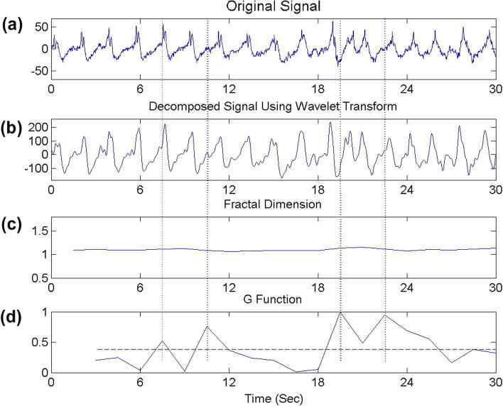
Fig. 9a shows the signal segmentation of a real EEG recording using the proposed method. Fig. 9b–d illustrates the signal after decomposing by five-level DWT, the FD of the decomposed signal and changes in the G function, respectively. It must be mentioned that these parameters are selected by trial and error.

Fig. 9.

Segmentation of real EEG data using the proposed method; (a) original signal, (b) decomposed signal after applying five-level DWT, (c) output of FD, and (d) G function result. It can be seen that all five segments can be accurately segmented.

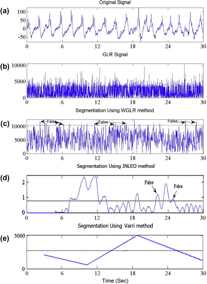
The signal in Fig. 9a is also segmented using four existing methods, namely, GLR [10], WGLR [10], INLEO [8], and Varri’s [22] methods in Fig. 10. It can be observed that the suggested method distinguishes the EEG signal segments better than the above existing methods.

Fig. 10.

Segmentation of real EEG using the existing methods; (a) original signal, (b) output of GLR method, (c) output of WGLR method, (d) output of INLEO method, and (e) output of Varri’s method.

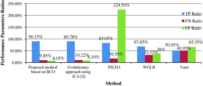
The simulation results of segmentation by using the proposed method with BCO are shown in Fig. 11. They indicate that the proposed method with BCO, compared with the three other well-known existent methods, has a better performance for segmenting the synthetic signals as well as real EEG data. This figure reveals that BCO has higher accuracy compared to the three existing methods. Albeit the INLEO method has adequate true positive ratios, its false positive ratios are the highest ones. Thus, the INLEO method has low reliability and it may not be appropriate for segmentation of real EEG signals. Furthermore, neither WGLR nor Varri’s methods have acceptable true positive ratios and false positive ratios. Hence, they are not considered reliable. Moreover, as can be seen in Fig. 11, in terms of all three parameters (TP, FN, and FP) by using real EEG signals, the proposed method is slightly better than the best approach proposed by Azami et al. [2].

Fig. 11.

Result of the suggested method with BCO when compared with evolutionary approach based on ICA [2], INLEO [8], WGLR [10] and Varri’s [22] methods, when applied to 40 real EEG datasets.

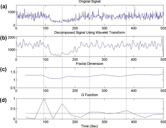
In Fig. 12, the proposed non-stationary signal segmentation is assessed by the difference of the real photons’ arrival rates. Fig. 12b–d respectively illustrate the signal after decomposing by three-level DWT, the FD of the decomposed signal, and changes in the G function.

Fig. 12.

Segmentation of the difference signal of the real photons arrival rates using the proposed method; (a) original signal, (b) decomposed signal after applying three-level DWT, (c) output of FD, and (d) G function result. It can be seen that all five segments can be accurately detected.

To comprehend the performance of the suggested method, first, Fig. 12a illustrates the difference between the real photons’ rates, as in Fig. 4b. This signal is segmented using four existing methods, namely, GLR [10], WGLR [10], INLEO [8] and Varri’s [22] methods in Fig. 13. It can be observed that the proposed approach by using BCO distinguishes the real signal segments better than attained outputs by the existing methods.

Fig. 13.

Segmentation of the difference signal of the real photons’ arrival rates using the existing methods: (a) original signal, (b) output of GLR method, (c) output of WGLR method, (d) output of Varri’s method, and (e) output of INLEO method.

In Fig. 12a, in the first segment signal has a smooth variation. The amplitude in the first part of the second segment begins to rises and it is dissimilar in the second segment, whereas in the 3rd segment the amplitude of the signal increases. As it can be seen in this figure, the 4th and 5th segments have different frequencies. When the input signal is collected from person’s body, the above perception can help the physiologists to distinguish when a disorder or an abnormality manifests itself.

Conclusions

In this article an adaptive segmentation approach using DWT, FD and EAs has been proposed. The DWT has been used to obtain a more informative multiresolution representation of a signal which is very valuable in detection of abrupt changes within that signal. The changes in FD refer to the underlying statistical variations in the signals and time series, such as the transients and sharp changes, in both the frequency and amplitude. There are two parameters that influence the boundaries and control the accuracy of the signal segmentation. In order to attain the acceptable values of these parameters, we have used four EAs, namely, PSO, NPSO, the improved PSO with mutation and BCO. The results of applying the suggested methods, tested on synthetic signal, real EEG data, and brightness changes in galactic objects, have indicated the higher performance of the methods compared with three existing non-evolutionary methods, namely, WGLR, Varri’s and INLEO as well as three evolutionary approaches based on the FD.

Conflict of interest

The authors have declared no conflict of interest.

Compliance with Ethics Requirements

This article does not contain any studies with human or animal subjects.

References

- 1.Scargle J.D. Studies in astronomical time series analysis. V. Baysian blocks, a new method to analyze structure in photon counting date. Astron J. 1998;504:405–418. [Google Scholar]
- 2.Azami H., Sanei S., Mohammadi K., Hassanpour H. A hybrid evolutionary approach to segmentation of non-stationary signals. Digital Signal Proc. 2013;23(4):1103–1114. [Google Scholar]
- 3.Sanei S., Chambers J. John Wiley & Sons; 2007. EEG signal processing. [Google Scholar]
- 4.Anisheh S.M., Hassanpour H. Adaptive segmentation with optimal window length scheme using fractal dimension and wavelet transform. Int J Eng. 2009;22(3):257–268. [Google Scholar]
- 5.Wang D, Vogt R, Mason M, Sridharan S. Automatic audio segmentation using the generalized likelihood ratio. In: 2nd IEEE international conference on signal processing and communication systems; 2008. p. 1–5.
- 6.Lv J, Li X, Li T. Web-based application for traffic anomaly detection algorithm. In: Second IEEE international conference on internet and web applications and services; 2007. p. 44–60.
- 7.Agarwal R, Gotman J. Adaptive segmentation of electroencephalographic data using a nonlinear energy operator. In: IEEE international symposium on circuits and systems (ISCAS’99), vol. 4; 1999. p. 199–202.
- 8.Hassanpour H, Shahiri M. Adaptive segmentation using wavelet transform. In: International conference on electrical engineering; 2007. p. 1–5.
- 9.Gao J., Sultan H., Hu J., Tung W.W. Denoising nonlinear time series by adaptive filtering and wavelet shrinkage: a comparison. IEEE Signal Process Lett. 2010;17(3):237–240. [Google Scholar]
- 10.Cappé O., Moulines E., Ryden T. Springer-Verlag; 2005. Inference in hidden Markov models. [Google Scholar]
- 11.Lanchantin P., Lapuyade-Lahorgue J., Pieczynski W. Unsupervised segmentation of randomly switching data hidden with non-Gaussian correlated noise. Signal Process. 2011;91(2):163–175. [Google Scholar]
- 12.Falconer J. John Wiley and Sons; New York, U.S.A: 2003. Fractal geometry mathematical foundations and applications. [Google Scholar]
- 13.Tao Y., Lam E.C.M., Tang Y.Y. Feature extraction using wavelet and fractal. Elsevier J Pattern Recogn. 2001;22(3–4):271–287. [Google Scholar]
- 14.Gunasekaran S, Revathy K. Fractal dimension analysis of audio signals for Indian musical instrument recognition. In: International conference on audio, language and image processing (ICALIP); 2008. p. 257–61.
- 15.Esteller R., Vachtsevanos G., Echauz J., litt B. A comparison of waveform fractal dimension algorithms. IEEE Trans Circ Syst. 2001;48(2):177–183. [Google Scholar]
- 16.Kennedy J, Eberhart R. Particle swarm optimization. In: IEEE conference on neural networks; 1995. p. 1942–8.
- 17.Yang C, Simon D. A new particle swarm optimization technique. In: International conference on systems engineering; 2005. p. 164–9.
- 18.Karaboga N. A new design method based on artificial bee colony algorithm for digital IIR filters. J Franklin Inst. 2009;346(4):328–348. [Google Scholar]
- 19.Karaboga D., Akay B. A comparative study of artificial bee colony algorithm. Appl Math Comput. 2009;214(1):108–132. [Google Scholar]
- 20.Karaboga D., Basturk B. A powerful and efficient algorithm for numerical function optimization: artificial bee colony (ABC) algorithm. J Glob Opt. 2007;39(3):459–471. [Google Scholar]
- 21.Azami H., Khosravi A., Malekzadeh M., Sanei S. A new adaptive signal segmentation approach based on Higuchi’s fractal dimension. vol. 304. Springer Verlag; 2012. (Communications in computer and information science). p. 152–9. [Google Scholar]
- 22.Krajca V., Petranek S., Patakova I., Varri A. Automatic identification of significant grapholements in multichannel EEG recordings by adaptive segmentation and fuzzy clustering. Int J Bio-Med Comput. 1991;28(1–2):71–89. doi: 10.1016/0020-7101(91)90028-d. [DOI] [PubMed] [Google Scholar]