Deformation field correction for spatial normalization of PET images

Abstract

Spatial normalization of positron emission tomography (PET) images is essential for population studies, yet the current state of the art in PET-to-PET registration is limited to the application of conventional deformable registration methods that were developed for structural images. A method is presented for the spatial normalization of PET images that improves their anatomical alignment over the state of the art. The approach works by correcting the deformable registration result using a model that is learned from training data having both PET and structural images. In particular, viewing the structural registration of training data as ground truth, correction factors are learned by using a generalized ridge regression at each voxel given the PET intensities and voxel locations in a population-based PET template. The trained model can then be used to obtain more accurate registration of PET images to the PET template without the use of a structural image. A cross validation evaluation on 79 subjects shows that the proposed method yields more accurate alignment of the PET images compared to deformable PET-to-PET registration as revealed by 1) a visual examination of the deformed images, 2) a smaller error in the deformation fields, and 3) a greater overlap of the deformed anatomical labels with ground truth segmentations.

1. Introduction

Deformable medical image registration is an indispensable tool for neuroimaging research. It is essential to the tasks of aligning a population of images, performing voxelwise association studies to identify subtle differences across groups, and tracking longitudinal changes. While within-modality spatial normalization of structural medical images has been studied extensively, work on anatomically accurate positron emission tomography (PET) spatial normalization without the use of a corresponding structural image remains limited. The anatomical alignment of PET images is a difficult problem since they reflect metabolism and function rather than anatomy, the observed intensities depend on the amount of radiotracer used, and the spatial detail is confounded by radiotracer spillover.

Prior studies on PET registration have shown that using a corresponding MRI to perform spatial normalization allows for better detection of disease-related changes (Martino et al., 2013). Therefore, whenever available, it is preferable to use a structural image (such as a T₁-weighted MRI) co-registered with the subject’s PET image for registration purposes to warp the PET image accordingly. However, it is important to be able to perform PET spatial normalization accurately without guidance from additional images, as structural MR images are not always available due to claustrophobia or MR-incompatible implants (Merrill et al., 2012; Morbelli et al., 2010). For example, the Australian Imaging Biomarkers and Lifestyle (AIBL) study does not include MR imaging for 20% of their PET participants (Bourgeat et al., 2015). Additionally, MR scans might have to be excluded in PET studies due to inadequate quality (Karow et al., 2010) or due to protocol or scanner changes over the course of a longitudinal study. These missing MR scans require the exclusion of subjects who otherwise have complete data in PET studies where MR images are used to perform spatial normalization or anatomical segmentation (Ciarmiello and Cannella, 2006). Given the relatively small samples in PET studies, it is important to include as many subjects as possible in statistical analyses to prevent reductions in power.

Prior work on PET spatial normalization includes using existing registration algorithms in conjunction with PET templates specifically designed for the relevant radiotracer (Zamburlini et al., 2004; Della Rosa et al., 2014), modification of the target image intensities using a whole-brain principal component analysis (Fripp et al., 2008a) or a linear regression (Lundqvist et al., 2013; Thurfjell et al., 2014) model to match more closely to the moving image intensities, and additionally imposing constraints on the PET deformations in the registration via a statistical control point model based on the deformation parameters of PET-to-MR registrations (Fripp et al., 2008b). Another approach to PET spatial normalization is making use of the 4D data available in dynamic PET studies (Bieth et al., 2013). While these approaches show improvements over ordinary 3D PET spatial normalization, they do not make use of a unified population model of PET intensities and deformations. The method proposed by Bieth et al. (2013) is a 4D extension of 3D PET-to-PET registration, and is still susceptible to the systematic errors present in PET-to-PET registration due to the incorrect inference of anatomical boundaries stemming from spillover effects and the preferential binding of the radiotracer to certain parts within structures. The method proposed by Fripp et al. (2008b) does use population models of PET intensities as well as deformations; however, the intensity and deformation models are separate and influence each other only via an iterative framework. Other methods have been proposed to enable quantification of PET images in the absence of a corresponding MRI, but do not involve performing spatial normalization. Such methods include Zhou et al. (2014) and Bourgeat et al. (2012, 2015).

We present a method for the spatial normalization of PET images based on a deformation correction model learned from structural image registration. Our method constructs a unified population model of both PET intensities and deformations in order to correct the PET registration. This paper extends our previous approach for deformation field correction by incorporating a spatial smoothness constraint and performing a more extensive validation of the proposed method (Bilgel et al., 2014). The observation motivating our method is: PET-to-PET registration produces deformations that are systematically biased in certain regions, and these biases can be characterized as a function of location. These biases are illustrated in Fig. 1, which shows an average of MRIs warped according to MR-to-MR template deformations and according to PET-to-PET template deformations. This comparison shows that the ventricles as well as subcortical gray matter structures are smaller in PET-to-PET registration, and that the biases in PET-to-PET registration are dependent on spatial position. We present a correction that operates on the PET-to-PET deformation fields obtained from a deformable registration algorithm and uses generalized ridge regression models learned from a population of subjects relating the local PET intensities and deformation fields to the corresponding structural imaging deformation fields. The learned relationship between the deformation fields accounts for the anatomical inaccuracies present in the alignment of PET images, while the use of PET intensity information allows for inter-subject variability in radiotracer binding due to differences in physiology. Our method can be applied to results obtained with any deformable registration algorithm.

Figure 1.

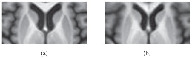
Average of MRIs warped according to (a) MR-to-MR template deformations and (b) PET-to-PET template deformations.

2. Material and Methods

2.1. Participants

We used imaging data from 94 participants from the Baltimore Longitudinal Study of Aging (BLSA) (Shock et al., 1984) neuroimaging substudy (Resnick et al., 2000). At enrollment into the neuroimaging substudy, participants were free of central nervous system disease, severe cardiac disease, severe pulmonary disease, or metastatic cancer. A subset of the BLSA neuroimaging participants received positron emission tomography (PET) scans obtained with the radiotracer Pittsburgh compound B (PiB) beginning in 2005. 3 of the 94 participants had diagnoses of mild cognitive impairment (MCI) and one had a diagnosis of Alzheimer’s disease (AD). The remaining individuals were cognitively normal. Diagnoses of dementia and AD were based on DSM-III-R (American Psychiatric Association, 1987) and the NINCDS-ADRDA criteria (McKhann et al., 1984). The image data consists of both structural images, which are 3T MPRAGE magnetic resonance images, and PET images obtained with the radiotracer PiB (PiB-PET), which are representative of the fibrillar β-amyloid distribution. The 94 subjects were separated into two mutually exclusive groups. Fifteen were designated as “template subjects” and used to generate the image templates as described below in §2.4, and the remaining 79 were designated as “validation subjects” and used for model training and testing (§2.6–2.7). The two groups had similar age distributions and a balanced representation of males and females. The percentage of individuals with elevated levels of amyloid was similar across the two groups. Participant demographics are presented in Table 1.

Table 1.

Demographics for the participants used for template generation and for bmethod validation.

	Template subjects	Validation subjects
Sample size	15	79
Age, mean yrs ± SD	80.4 ± 8.8	77.1 ± 8.3
Male, N (%)	8 (53.3%)	39 (49.4%)
High PiB, N (%)	4 (26.7%)	22 (27.8%)

2.2. Image acquisition

PET scans were acquired on a GE Advance scanner immediately following an intravenous bolus injection of Pittsburgh compound B (PiB), which binds to fibrillar β-amyloid. Dynamic PET data were acquired over 70 minutes, yielding 33 time frames each with 128×128×35 voxels. Dynamic images were constructed using filtered backprojection with a ramp filter, yielding a spatial resolution of approximately 4.5 mm FWHM at the center of the field of view. Voxel size was 2 × 2 × 4.25 mm³. For registration purposes, we obtained static images by averaging the time frames of the dynamic scan. Many PiB-PET studies acquire static scans 40–60 or 50–70 minutes post injection. As suggested by McNamee et al. (2009), the four time frames corresponding to 50–70 minutes were averaged to create a static PET image. Since the 50–70 minute average contains β-amyloid information that can vary greatly across subjects, we also averaged the first 23 time frames corresponding to the first 20 minutes to create a 20-minute mean PET image for each subject. Early time frames were chosen as they are mostly reflective of cerebral blood flow and show clearer anatomic boundaries less vulnerable to modification by β-amyloid.

For structural images, we used MPRAGE scans acquired on a Philips Achieva 3T scanner with the following acquisition parameters: TR = 6.8 ms, TE = 3.2 ms, α = 8° flip angle, 256 × 256 matrix, 170 sagittal slices, 1 × 1 mm² in-plane pixel size, 1.2 mm slice thickness.

The MPRAGE scans of two subjects used for template construction and four subjects used for cross-validation were not concurrent with their PET scans. The average interval between these non-concurrent scans for the template and cross-validation subjects were 2.89 and 3.08 years, respectively. The remaining subjects had both scans at the same visit.

2.3. Image preprocessing

After intensity inhomogeneity correction (Sled et al., 1998), the structural images S_i : Ω_Si → ℝ, where Ω_Si is the domain of image S_i, were co-registered rigidly with their corresponding PET images F_i : Ω_Fi → ℝ for each subject i, yielding the transformation R_i : ℝ³ → ℝ³. The aligned structural images were then skull-stripped (Carass et al., 2011). Skull-stripping the MR and PET images prior to co-registration resulted in less accurate registration of the brain boundary, and therefore was not performed. Preprocessing was conducted using the Java Image Science Toolkit (JIST) (Lucas et al., 2010).

2.4. Image template generation

The generation of the image templates is summarized in Fig. 2. To create an anatomically accurate PET template image, we relied on the associated structural images. We used the ANTs package (http://picsl.upenn.edu/software/ants/) (Avants et al., 2011) to construct the population templates. Specifically, the skull-stripped structural images for the n = 15 template subjects were affinely registered to a common space with transformation T_i : ℝ³ → ℝ³, where i is in the set of template subjects Γ_temp. The affinely coregistered structural images Ŝ_i = S_i (R_i ∘ T_i) were then used to create a structural population template image S̄. Let x be in the common space Ω, and ϕ_i a diffeomorphism defined on Ω × to transform Ŝ_i into a new coordinate system by Ŝ_i ∘ ϕ_i(x, t), with t ∈ = [0, 1] and ϕ_i(x, 0) = x. For simplicity, we denote the full diffeomorphism ϕ_i(x, 1) between the moving and the target images as ϕ_i(x), or equivalently as ϕ_i. The square-integrable and continuous vector field ν_i(x, t) parameterizes the diffeomorphism such that $\frac{d{\mathit{\varphi }}_i(\mathit{x},t)}{dt}={\mathit{\nu }}_i({\mathit{\varphi }}_i(\mathit{x},t),t)$ (Avants et al., 2008). The population template S̄ was obtained using the equation

Figure 2. Image template generation.

The structural images S_i (i ∈ Γ_temp) are first co-registered with their corresponding PET images F_i, and then used to construct the population-average structural image template S̄ using a deformable registration framework. The resulting mappings T_i ∘ ϕ_i are applied to the PET images. The deformed PET images are averaged to construct the PET image template F̄.

$$\overline{S},\{{\mathit{\varphi }}_i\}=\underset{\overline{S},\{{\mathit{\varphi }}_i\}}{argmin}\sum _{i\in {\mathrm{\Gamma }}_{\text{temp}}}\left({\int }_0^1{\Vert {\mathit{\nu }}_i(\mathit{x},t)\Vert }_L^{2}dt+{\int }_{\mathrm{\Omega }}-\text{CC}\left(\overline{S},{\widehat{S}}_i({\mathit{\varphi }}_i),\mathit{x}\right)d\mathrm{\Omega }\right),$$ (1)

where L is a Gaussian convolution operator regularizing the velocity field, and CC(S̄, Ŝ_i(ϕ_i), x) is the cross correlation (CC) similarity measure with the inner products calculated over a cubic window around x (Avants et al., 2010).

The affine transformations T_i and diffeomorphisms ϕ_i obtained from the structural image template construction were applied to the corresponding PET images in order to bring them into the same template space. The PET template F̄ was then defined as the mean of the spatially normalized PET images as

$$\overline{F}=\frac{1}{n}\sum _{i\in {\mathrm{\Gamma }}_{\text{temp}}}{F}_i({\mathit{T}}_i,\circ {\mathit{\varphi }}_i).$$ (2)

PET images were resampled as part of the registration algorithm used for spatial normalization to yield registered images with 1 mm isotropic voxels.

2.5. Computing a training set

The training set computation procedure is summarized in Fig. 3. We performed deformable registration to map the PET images onto the PET template using SyN (Avants et al., 2008). For each subject i among the 79 validation subjects, the deformable registration consisted of an affine transformation ${\mathit{T}}_i^{\prime }$ followed by a diffeomorphic mapping ψ_i = ψ_i(x, 1) defined on Ω. We denote the PET image registered onto the PET template F̄ by ${\stackrel{\sim }{F}}_i=F_i({\mathit{T}}_i^{\prime }\circ {\mathit{\psi }}_i)$. Constraining the affine transformation to be the same as that obtained from the PET-to-PET registration, we then performed another registration to find the deformation field ξ_i that must be applied to the structural image such that ${\stackrel{\sim }{S}}_i=S_i({\mathit{R}}_i\circ {\mathit{T}}_i^{\prime }\circ {\mathit{\xi }}_i)$ is in alignment with the structural image template S̄. We used the same registration parameters for the alignment of PET and structural images. All transformations and deformations were concatenated and images were interpolated only once going from their native spaces to the template space according to this concatenated mapping. The validation subjects are used in 10-fold cross validation as described in §2.11. For each fold of the cross validation, a subset of the validation subjects are selected as training subjects, and the remainder are testing subjects.

Figure 3. Computing a training set.

The PET images F_i (where i is in the set of training subjects) are deformably registered onto the PET template F̄. The structural images S_i are first co-registered with their corresponding PET images, followed by a deformable registration onto the structural image template S̄. The affine transformation ${\mathit{T}}_i^{\prime }$ preceding the deformation is constrained to be the affine transformation obtained from PET-to-PET template registration.

2.6. Model training

Our goal is to train a multivariate linear regression model at each voxel x ∈ Ω describing a relationship between the estimated PET deformation field ψ_i(x) and the structural image deformation field ξ_i(x), where i is a subject in the training set, for the m training subjects. The independent variables in the model include intercept, the PET deformation field, and the PET intensities F̄_i(x) in the common space Ω. These intensities are included to account for the variability in PET intensities across subjects due to differences in function and metabolism. The independent variables make up the matrix X, which consists of input features compiled across the m subjects:

$$\mathbf{X}(\mathit{x})=\left[\begin{array}{ccc}⋮& ⋮& ⋮\\ 1& {\mathit{\psi }}_i(\mathit{x})& {\stackrel{\sim }{F}}_i(\mathit{x})\\ ⋮& ⋮& ⋮\end{array}\right]\in {ℝ}^{m\times 5}.$$ (3)

The dependent variable is the structural image deformation field, yielding the output matrix Y, which consists of data compiled across the m subjects:

$$\mathbf{Y}(\mathit{x})=\left[\begin{array}{c}⋮\\ {\mathit{\xi }}_i(\mathit{x})\\ ⋮\end{array}\right]\in {ℝ}^{m\times 3}.$$ (4)

The multivariate linear regression model is

$$\mathbf{Y}=\mathbf{XB}+\mathit{\epsilon },$$ (5)

where ε ~ (0, Σ) is the noise term. The least squares estimate of the regression coefficient B ∈ ℝ^5×3 of the multivariate linear regression model is found by minimizing the cost function

$$Q(\mathbf{B})=\text{tr}\left[{(\mathbf{Y}-\mathbf{XB})}^T(\mathbf{Y}-\mathbf{XB})\right],$$ (6)

which yields the estimate

$$\widehat{\mathbf{B}}={({\mathbf{X}}^T\mathbf{X})}^{-1}{\mathbf{X}}^T\mathbf{Y}$$ (7)

for the regression coefficient matrix. The estimate of the covariance is then given by

$$\widehat{\mathbf{\sum }}={(\mathbf{Y}-\mathbf{X}\widehat{\mathbf{B}})}^T(\mathbf{Y}-\mathbf{X}\widehat{\mathbf{B}})/(m-p),$$ (8)

where p = 5 is the number of columns of X. However, the regression coefficients estimated using such an approach are not necessarily smooth since each voxel is processed independently. We describe an approach for obtaining spatially smooth estimates in the following section.

2.7. Spatial smoothness

We seek to obtain smooth estimates for the coefficient matrix B since nearby voxels are likely to have similar relationships between the structural and PET images. Furthermore, smooth coefficient matrices, when applied to diffeomorphic PET deformation fields, will yield smoother predicted deformation fields, which is a desirable feature.

Obtaining smooth estimates for the coefficient matrix amounts to reducing the variability associated with the coefficients while introducing a bias towards a smoother set of estimates. To achieve this, we employ generalized ridge regression (GRR), which involves adding a regularizing term to the cost function of the linear regression model. This term penalizes estimates that are not close enough to a set of a priori expected values for the regression coefficients (Hoerl and Kennard, 1970a,b). In the multivariate outcome case (Brown and Zidek, 1980), we denote the a priori expected value of the regression coefficient matrix as B₀, which in our application will be chosen to be a spatially smooth version of the ordinary least squares estimate B̂. We also define a priori a matrix H, which allows for controlling the influence of the regularization term on each element of the regression coefficient matrix. The original cost function (Eq. 6) is modified to yield the multivariate GRR cost function:

$$Q(\mathbf{B};\mathbf{H})=\text{tr}[{(\mathbf{Y}-\mathbf{XB})}^T(\mathbf{Y}-\mathbf{XB})+{(\mathbf{B}-{\mathbf{B}}_{\mathbf{0}})}^T\mathbf{H}(\mathbf{B}-{\mathbf{B}}_{\mathbf{0}})].$$ (9)

By taking the derivative of Q(B; H) with respect to B and setting it to zero, we obtain that the regression coefficient estimate is given by

$${\widehat{\mathbf{B}}}^{\ast }={({\mathbf{X}}^T\mathbf{X}+\mathbf{H})}^{-1}({\mathbf{X}}^T\mathbf{Y}+{\mathbf{HB}}_0).$$ (10)

When H = 0, the solution is the same as the ordinary least squares solution, and as the diagonal entries of H tend to infinity, the regression coefficients approach the expected value B₀.

We spatially smooth the linear regression estimates calculated using Eq. (7) to obtain B₀. For each entry in B̂, we apply a 3-D Gaussian filter with standard deviation σ to smooth the regression coefficients across the brain voxels. The resulting smoothed values make up the matrix B₀.

We choose the diagonal entries of H for the multivariate case in a manner similar to the univariate case adopted by Zhou et al. (2001, 2003):

$$h_i=\frac{\alpha \text{tr}(\widehat{\mathbf{\sum }})}{{({\widehat{\mathbf{b}}}_i-{\mathbf{b}}_{i0})}^T({\widehat{\mathbf{b}}}_i-{\mathbf{b}}_{i0})},$$ (11)

where σ̂ is as in Eq. (8), and b̂_i and b_i0 are column vectors corresponding to the i^th row of the linear regression estimate B̂ and the expected value B₀, respectively. The parameter α allows for adjusting the weight on the second term in Eq. (9) relative to the first term. The regression coefficients obtained using Eq. (10) will be smoother than those obtained using Eq. (7). The GRR method was implemented in Matlab (Mathworks, Natick, MA) and is available upon request.

2.8. PET deformation field prediction

Once we have estimates for B̂^* at each voxel, given a PET image deformed onto the template and its associated deformation field, we can predict the structural image deformation field at each voxel x as ξ̂(x) = X(x)B̂^*(x), where X(x) is the input feature matrix for the PET image at voxel x, as defined previously. This allows for the prediction of the corrected deformation fields for performing registration onto the template for PET images that do not have a corresponding MRI.

2.9. Parameter tuning

To choose the ridge regression smoothness parameter α and the Gaussian smoothing parameter σ, we compared the root mean square (RMS) deformation field error over a cortical gray matter (GM) mask in a central axial slice for a range of α and σ values. We used the MPRAGE-to-MPRAGE deformations as ground truth for the error calculations. Each model was trained on 40 of the 79 validation subjects and tested on the remaining 39 for the purpose of parameter tuning.

2.10. PCA method

We compared our method against PET-to-PET template registration and an implementation of the method described by Fripp et al. (2008b). The Fripp et al. (2008b) method comprises first creating a PET template using corresponding MR images as in our approach and constructing a whole-brain principal component analysis (PCA) model from the spatially normalized PET image intensities. The subject’s PET is affinely registered onto the template, which is then modified using the PCA model to resemble more closely the subject. Finally, the subject’s PET is deformable registered onto the modified template. For consistency, we used SyN registration in our implementation of this method. Since SyN does not use B-splines, we did not implement the statistical control point model presented by Fripp et al. (2008b). We refer to our implementation of the method proposed by Fripp et al. (2008b) as the PCA method.

2.11. Method validation

We validated our ridge regression method and the PCA method using 10-fold cross validation on the 79 validation subjects. The cross validation involves using 9 of the 10 groups for model training, and testing this model on the remaining group. This is repeated until every group has been tested and a corrected PET deformation field has been obtained for each individual. The MRI-to-MRI registrations of the testing subjects were used to quantify prediction errors only, not in the deformation prediction itself. We randomly assigned the 79 participants to the cross validation groups. The prediction errors were quantified using the MR-based registration results of the test subjects. All of the following validation metrics were calculated in the 1 mm isotropic template space.

2.11.1. Visual comparison of deformation fields

For a visual comparison, each 0–20 minute PiB-PET and MPRAGE image was warped by the deformation fields obtained from the different methods based on 0–20 minute PiB-PET registration, and averaged across the 79 subjects to yield mean images.

2.11.2. RMS error of deformation fields

We computed the root mean square (RMS) error of the deformation field vectors at each voxel in the template space across 79 individuals, using the deformation field ξ obtained from the registration of MPRAGE onto the MPRAGE template as ground truth.

2.11.3. Dice coefficients

To assess the accuracy of anatomical alignment, the FreeSurfer (Dale et al., 1999; Desikan et al., 2006) segmentations of the original MPRAGE images were brought into the template space by applying the mappings from the previously performed registrations. Using the FreeSurfer labels deformed according to ξ as ground truth, we calculated the Dice coefficients (Dice, 1945) for the deformed labels.

3. Results

We investigated mutual information as a cost function for the spatial normalization of PiB-PET images with SyN and found that CC yields deformation fields with smaller root mean square (RMS) errors throughout the brain as compared to the MPRAGE-to-MPRAGE deformation fields (data not presented). Therefore, we used CC as the cost function in all SyN registrations.

3.1. Parameter tuning

The results for a selected set of α and σ values are presented in Fig. 4. Note that σ is not used in the registration, but rather in the multivariate GRR. It determines the level of smoothness to be imposed on the regression coefficients obtained from the GRR. The effect of α on the RMS error is dependent on σ. The lower bound on the RMS in Fig. 4 reflects the extent of the spatial correlation in the underlying regression coefficients. At small values of σ, the RMS error decreases monotonically as a function of α. However, at large values of σ, the RMS error begins to increase beyond a certain α threshold. These trends can be seen in Fig. 4. The improvement in picking the optimal values of α and σ is about 0.1 mm in RMS, with a range of parameter combinations yielding a comparable improvement. Therefore, the final performance of the algorithm does not hinge upon the precise selection of these two parameters. In the remainder of the experiments, we used α = 5 and σ = 10 mm for the 0–20 minute PiB-PET images, and α = 5 and σ = 8 mm for the 50–70 minute images as these values minimized the RMS error over the cortical GM mask.

Figure 4. Parameter tuning.

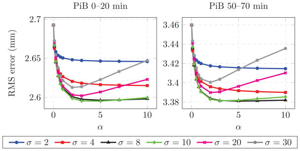
The root mean square (RMS) deformation field error (mm) over a cortical gray matter (GM) mask in a single axial slice through the center of the brain across the 39 testing subjects as a function of the ridge regression smoothness parameter α for different values of the Gaussian smoothing parameter σ (in mm). Left: Results for the 0–20 minute PiB-PET. Right: Results for the 50–70 minute PiB-PET. For references to color, the reader is referred to the web version of this article.

3.2. Method validation

3.2.1. Visual comparison of deformed images

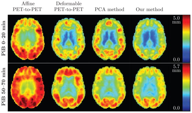
The average of the 0–20 minute PiB-PET and MPRAGE images warped by the deformation fields obtained from the different methods based on 0–20 minute PiB-PET registration are shown in Fig. 5. For visualization purposes, the histogram of each PET mean image was matched to that of the mean of the PET images deformed using the MPRAGE-to-MPRAGE deformation field (similarly for the MPRAGE images). We calculated the difference of each of the average deformed images and the ground truth image (average of the images deformed according to the MPRAGE-to-MPRAGE deformations) to obtain a clear depiction of the differences among the images.

Figure 5.

Deformed images averaged across 79 subjects for the 0–20 minute PiB-PET results. First row: Average of the PET images deformed using the deformation ξ from MPRAGE-to-MPRAGE template registration, the deformation ψ from PET-to-PET template registration, the deformation given by the PCA method, and the deformation ξ̂ predicted using our model. Second row: Average of the MPRAGE deformed using ξ, ψ, the deformation given by the PCA method, and ξ̂. Last two rows: Difference of each of the deformed images and the ground truth image (average of the images deformed according to the MPRAGE-to-MPRAGE deformation ξ).

PET-to-PET registration results in misaligned cortical GM, ventricles and subcortical GM structures. These effects can clearly be seen in the MPRAGE difference images of Fig. 5. The PCA method yields smaller differences around the ventricles and subcortical GM structures. Our method reduces these differences, and is also able to reduce the differences in parts of the cortical GM, most noticeably the insular cortex. While PET-to-PET deformation yields the sharpest PET mean image, it is not anatomically accurate as revealed by its difference with the ground truth. Our method reduces the differences for the mean PET images as well.

3.2.2. RMS error of deformation fields

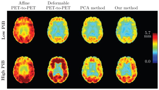
A comparison of the root mean square (RMS) error of the deformation fields is presented in Fig. 6, including the result of affine PET-to-PET registration as a baseline reference. The registration accuracy of the 0–20 minute PET is better than that of the 50–70 minute PET, with or without deformation field correction. The PCA method reduces the deformation errors for the 50–70 minute images, but exacerbates them for the 0–20 minute images. Our method achieves the lowest overall RMS error for both the 0–20 minute and 50–70 minute PiB-PET images.

Figure 6.

Root mean square (RMS) error (in mm) of the PET deformation fields obtained from different approaches, calculated across 79 subjects. An axial brain slice is shown. Top row: Results for 0–20 minute PiB-PET. Bottom row: Results for 50–70 minute PiB-PET. Left to right: RMS error of the affine PET-to-PET registration T′, RMS error of the PET-to-PET deformation ψ, RMS error of the deformation given by the PCA method, and RMS error of ξ̂ predicted using our model. For references to color, the reader is referred to the web version of this article.

3.2.3. Dice coefficients

For the 0–20 minute PiB-PET images, the Dice coefficients for our method are statistically different from deformable PET-to-PET registration for temporal gray matter (GM) (p = 0.005), insular GM (p < 0.001), ventricles (p < 0.001), thalamus-caudate-putamen (p < 0.001), and close to significance for occipital GM (p = 0.07). Our method is statistically different from the PCA method for all regions (p < 0.005). For the 50–70 minute PiB-PET images, the Dice coefficients for our method are statistically different from both deformable PET-to-PET registration and the PCA method for insular GM (p = 0.001 and p = 0.034, respectively) and thalamus-caudate-putamen (p = 0.002 and p = 0.024, respectively). The differences in the Dice coefficients for other regions did not reach significance. For both the 0–20 minute and 50–70 minute PiB-PET images, our method is statistically different from affine PET-to-PET registration for all regions.

4. Discussion

The 0–20 minute PiB-PET yielded more accurate registrations compared to the 50–70 minute PiB-PET, both with and without deformation correction. This highlights the importance of using the earlier time frames of the PiB-PET for registration purposes whenever available. The better performance of the 0–20 minute PET in registration might be in part attributed to its more pronounced gray-white matter contrast compared to the 50–70 minute PET. The intensity variability due to radiotracer binding is minimal on the 0–20 minute PiB-PET images, whereas the 50–70 minute images show great variability across subjects due to such differences, which negatively affects registration performance. Individuals with high levels of amyloid and thus greater radiotracer binding exhibit a different intensity profile on the 50–70 minute image than those with minimal amyloid. Such differences are not apparent on the 0–20 minute images since the PiB radiotracer is still in the uptake stage and the image largely reflects the distribution of the radiotracer due to circulation. This shows that correcting PET-to-PET registration is a greater concern when using 50–70 minute PiB-PET images. If a study requires PET-to-PET registration and corresponding MRIs are not acquired, then including the early time frames in the PET protocol should be considered, since registration correction methods on 50–70 minute images cannot achieve the level of registration accuracy obtained using 0–20 minute images.

The posterior brain regions exhibit relatively higher deformation field errors for both 0–20 and 50–70 minute images even after correction. This is most likely due to the complexity of the sulci and gyri in the posterior regions, and the lack of clear image features that can provide guidance for our correction model.

Given that the ground truth labels come from 1 × 1 × 1.2 mm³ structural images and our goal is to improve the registration of 2 × 2 × 4.25 mm³ PET images, it is inevitable that the improvements in Dice coefficients are very small, yet they are significant in several regions. The better performance of our method on the 0–20 minute images compared to the 50–70 minute images might be due to the more accurate PET-to-PET registration of the 0–20 minute images, which provides our method with a better starting point and as a result can yield more widespread improvements across the brain.

Our implementation of the PCA method proposed by Fripp et al. (2008b) can only account for intensity variations across subjects. This is illustrated by its lack of improvement on the 0–20 minute images but its significant reduction of registration error for the 50–70 minute images. Since our model aims to predict the structural deformation fields and does not rely solely on image intensities, it is able to improve both the 0–20 and 50–70 minute image registrations.

There are differences between the method proposed by Fripp et al. (2008b) and our implementation. While a free-form deformation method was used in Fripp et al. (2008b), we used a symmetric diffeomorphic registration method for consistency in comparison with our method. Furthermore, since the registration method we chose does not use B-splines, we were unable to incorporate the statistical control point models used in Fripp et al. (2008b) to further constrain the registration. Thus, we were unable to perform a direct comparison with the Fripp et al. (2008b) method. It is worth noting that the modeling of the deformation field and intensity information in the Fripp et al. (2008b) method are not coupled: Intensities are modified according to a PCA model that is uninformed about the local structure of the deformation field, and the regularization of the deformation field via the statistical control point model within the registration framework is uninformed about the PET intensity model. In our method, we use both the deformation field and the intensity information in a unified regression model as predictors, hence coupling the two sources of information in predicting the correct deformation field. We can only speculate about the potential improvements of such a coupling compared to the Fripp et al. (2008b) method. It is likely that our model provides a more accurate representation of the relationships between deformation field and PET intensity distributions, and as a consequence, would yield better results in data sets where such relationships are evident.

Our dataset contains a small number of individuals with elevated levels of PiB. The use of more than twice as many PiB− individuals compared to PiB+ in the training yields a model that is biased towards PiB− individuals. This is not a concern when using 0–20 minute images since they largely do not reflect amyloid distribution and are not highly variable across PiB− and PiB+ individuals. However, the composition of the training and testing sets in terms of amyloid positivity is a concern when using 50–70 minute PiB images. We have shown that even when the number of PiB− and PiB+ individuals are not balanced in the training sets, our model is able to reduce the RMS deformation field error across all individuals. With balanced datasets, the model could perform better due to the availability of more training data on PiB+ individuals.

Registration is a more challenging task in the presence of significant cortical atrophy that accompanies impairment. Since there was a limited number of individuals who were not cognitively normal in our dataset, we were unable to test our PET deformation correction method on images that contain high levels of atrophy and other neurodegenerative changes. Our findings may not extend to individuals who are at later stages of cognitive impairment and dementia, or who have cerebral malformations.

5. Conclusions

We presented a deformation correction method to improve the anatomical alignment of images in PET-to-PET registration. Deformable PET-to-PET registration results in systematic registration errors, especially when the activity patterns of the moving and the fixed images are different. Our method can compensate for such errors in PET-to-PET registration by learning locally from the structural image registrations. We demonstrated using cross-validation that our deformation correction method reduces the deformation field error and improves the anatomical alignment of PET images as evidenced by the higher Dice coefficients calculated using the deformed segmentations. While we used SyN for registration purposes, the method can be applied to any deformable PET-to-PET registration method. Furthermore, our method could also be extended to PET images involving radiotracers other than PiB.

Our method is particularly suited for spatial normalization of PET images in datasets where only a subset of the subjects have structural images. Subjects with both PET and structural images can be used to train the model, and those with only PET images can then be registered onto the PET template, taking into account the deformation correction provided by the model. If the dataset contains no concurrent PET and structural images, our deformation correction can still be applied given a PET template and an associated deformation field correction model that has already been constructed using a separate dataset.

The proposed approach could be extended beyond PET images and applied to improve the deformable registration of other types of medical images with low resolution, poor contrast, geometric distortions, or inadequate anatomical content by using a model trained on corresponding medical images that are largely free of such effects.

Highlights.

• We present a registration correction method for spatial normalization of PET images.

• The method is trained on data with both PET and structural images.

• Correction factors are learned using a generalized ridge regression at each voxel.

• Validation on 79 participants shows that our method yields more accurate alignment.

• Our method enables PET spatial normalization when structural images are unavailable.

Appendix A

RMS error of deformation fields by PiB group

We present the root mean square (RMS) error of the PET deformation fields separately for individuals with minimal or no amyloid (low PiB group) and with elevated levels of amyloid (high PiB group) for the 0–20 minute PiB-PET registrations in Fig. A.1, and for the 50–70 minute PiB-PET registrations in Fig. A.4. The RMS error calculation is the same as described in the main text for Fig. 6, except that we report RMS error separately for the two PiB groups.

Dice coefficients by PiB group

We present the Dice coefficient box plots by PiB group for the 0–20 minute and 50–70 minute PiB-PET registrations in Figs. A.2 and A.5, respectively. The Dice coefficients were calculated in the same manner as described in the main text for Fig. 7, except that we report the box plots separately for the two PiB groups.

Figure 7.

Box plots of Dice coefficients for cortical labels across 79 subjects calculated using the deformations obtained from affine PET-to-PET registration (red), deformable PET-to-PET registration (blue), the PCA method (green), and our method (purple). Statistically significant differences between our method and affine PET-to-PET registration, deformable PET-to-PET registration, and the PCA method are indicated with red, blue, and green asterisks, respectively (* : p < 0.05, ** : p < 0.01). For references to color, the reader is referred to the web version of this article.

Mean cortical SUVR

We investigated mean cortical standardized uptake value ratio (SUVR) values, which is a summary measure used to quantify levels of overall cerebral amyloid. The 50–70 minute PiB-PET images were brought into the template space by applying the mappings from the deformable PET-to-PET registration, the PCA method, and our method. We used FreeSurfer to segment the MPRAGE template. We used the cerebellar gray matter as the reference region to compute voxelwise SUVR. We computed the mean cortical SUVR as the average of values across frontal, parietal, lateral temporal and lateral occipital cerebral cortex (excluding the sensorimotor strip) using the 50–70 minute PiB-PET images. The mean cortical SUVRs calculated using PiB-PET images deformed according to the MRI-to-MRI mappings were considered as ground truth. Bland-Altman plots for mean cortical SUVR calculated based on 0–20 and 50–70 minute PiB-PET registrations are presented in Figs. A.3 and A.6, respectively.

It is worth noting that SUVR quantification depends on the correct placement of anatomical labels on the PET image and does not necessarily require spatial normalization. We did not optimize the placement of the anatomical labels and instead used the template labels for each spatially normalized PET image. There are methods designed specifically for SUVR quantification from PET images in the absence of corresponding MRIs, and they involve a labeling strategy to optimize SUVR computation (Bourgeat et al., 2012; Zhou et al., 2014). Since our main focus in this paper was not SUVR quantification but rather spatial normalization of PET images, we did not compare our approach to these methods.

Results based on 0–20 minute PiB-PET registration

The RMS error is higher among PiB+ individuals within each spatial normalization approach. Our method achieves the smallest RMS deformation field error in both the PiB− and the PiB+ group (Fig. A.1).

All brain regions included in the Dice coefficient analyses have significantly higher Dice coefficients as a result of our method compared to the PCA method in the PiB− group (Fig. A.2). Temporal and insular GM, ventricles, subcortical GM structures, and cerebellum show statistically significant improvements due to our method compared to deformable PET-to-PET registration in the PiB− group. On the other hand, in the PiB+ group, only the cerebral WM shows a statistically significant improvement in Dice coefficient as a result of our method compared to the PCA method. While there is a trend toward higher Dice coefficients in our method, no region shows a statistically significant improvement compared to deformable PET-to-PET registration in the PiB+ group.

The Bland-Altman plots of mean cortical SUVR for the different approaches are highly similar. All approaches yield unbiased mean cortical SUVR estimates, as evidenced by the mean difference close to 0 for all mean cortical SUVR levels. Our method has the smallest 95% confidence interval (Fig. A.3).

Results based on 50–70 minute PiB-PET registration

The RMS deformation field error is higher in the PiB+ group compared to the PiB− group within each spatial normalization approach (Fig. A.4). Among the PiB− individuals, our method yields the smallest RMS error. The difference between PiB+ and PiB− individuals is remarkable for deformable PET-to-PET registration. Except for in the ventricles, deformable PET-to-PET registration does very poorly in the PiB+ group, and yields higher RMS errors in most of the brain compared to affine PET-to-PET registration. The PCA method and our method remarkably reduce the RMS error in the PiB+ group, with the PCA method performing better overall.

Temporal and insular GM, subcortical GM structures and cerebellar GM show statistically significant improvements due to our method compared to deformable PET-to-PET registration in the PiB− group (Fig. A.5). Subcortical GM structures and cerebellar GM also show statistically significant improvements due to our method compared to the PCA method in the PiB− group. No region shows a statistically significant difference compared to the PCA method in the PiB+ group. Insular GM and subcortical GM structures have Dice coefficients that are statistically significantly better as a result of our method compared to deformable PET-to-PET registration.

While our method performs better than deformable PET-to-PET registration in computing mean cortical SUVR, it does not perform as well as the PCA method (Fig. A.6). Our method achieves a lower variability in the difference among the PiB− individuals compared to the PCA method.

It is possible that training our PET deformation field correction model based on the 50–70 minute PiB-PET images requires a larger dataset than the model based on the 0–20 minute images due to the higher variability present across individuals. In particular, the number of PiB+ individuals in the training sets might be insufficient to accurately train the GRR model. This could explain the better performance of our method compared to the PCA method among PiB+ individuals for the 0–20 minute images, but not for the 50–70 minute images.

Figure A.1.

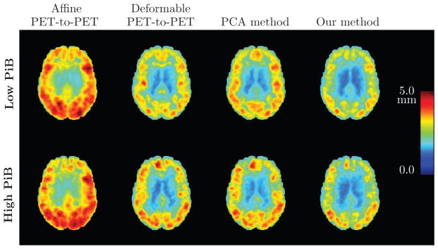
Root mean square (RMS) error (in mm) of the PET deformation fields obtained from different approaches based on 0–20 minute PiB-PET registration, calculated across 79 subjects. An axial brain slice is shown. Top row: Results for low PiB individuals. Bottom row: Results for high PiB individuals. Left to right: RMS error of the affine PET-to-PET registration T′, RMS error of the PET-to-PET deformation ψ, RMS error of the deformation given by the PCA method, and RMS error of ξ̂ predicted using our model.

Figure A.2.

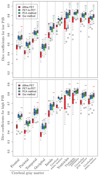
Box plots of Dice coefficients for cortical labels across 79 subjects calculated using the deformations obtained from affine PET-to-PET registration (red), deformable PET-to-PET registration (blue), the PCA method (green), and our method (purple) based on the 0–20 minute PiB-PET. Statistically significant differences between our method and affine PET-to-PET registration, deformable PET-to-PET registration, and the PCA method are indicated with red, blue, and green asterisks, respectively (* : p < 0.05, ** : p < 0.01).

Figure A.3.

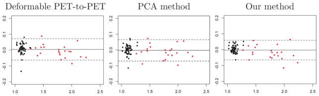
Bland-Altman plots for mean cortical SUVR calculated using 50–70 minute time frames registered based on 0–20 minute PiB-PET. The horizontal axis shows the mean of the measured mean cortical SUVR and the ground truth, and the vertical axis shows the difference between the two. The solid horizontal line corresponds to the mean difference, and the dashed lines indicate its 95% confidence interval. Black and red data points correspond to PiB− and PiB+ individuals, respectively.

Figure A.4.

Root mean square (RMS) error (in mm) of the PET deformation fields obtained from different approaches based on 50–70 minute PiB-PET registration, calculated across 79 subjects. An axial brain slice is shown. Top row: Results for low PiB individuals. Bottom row: Results for high PiB individuals. Left to right: RMS error of the affine PET-to-PET registration T′, RMS error of the PET-to-PET deformation ψ, RMS error of the deformation given by the PCA method, and RMS error of ξ̂ predicted using our model.

Figure A.5.

Box plots of Dice coefficients for cortical labels across 79 subjects calculated using the deformations obtained from affine PET-to-PET registration (red), deformable PET-to-PET registration (blue), the PCA method (green), and our method (purple) based on the 50–70 minute PiB-PET. Statistically significant differences between our method and affine PET-to-PET registration, deformable PET-to-PET registration, and the PCA method are indicated with red, blue, and green asterisks, respectively (* : p < 0.05, ** : p < 0.01).

Figure A.6.

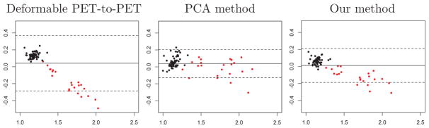
Bland-Altman plots for mean cortical SUVR calculated using 50–70 minute time frames registered based on 50–70 minute PiB-PET. The horizontal axis shows the mean of the measured mean cortical SUVR and the ground truth, and the vertical axis shows the difference between the two. The solid horizontal line corresponds to the mean difference, and the dashed lines indicate its 95% confidence interval. Black and red data points correspond to PiB− and PiB+ individuals, respectively.

References

- American Psychiatric Association. Diagnostic and Statistical Manual of Mental Disorders: DSM-III-R. 4. Washington, DC: 1987. [Google Scholar]
- Avants BB, Epstein CL, Grossman M, Gee JC. Symmetric diffeomorphic image registration with cross-correlation: evaluating automated labeling of elderly and neurodegenerative brain. Medical Image Analysis. 2008;12:26–41. doi: 10.1016/j.media.2007.06.004. [DOI] [PMC free article] [PubMed] [Google Scholar]
- Avants BB, Tustison NJ, Song G, Cook PA, Klein A, Gee JC. A reproducible evaluation of ANTs similarity metric performance in brain image registration. NeuroImage. 2011;54:2033–2044. doi: 10.1016/j.neuroimage.2010.09.025. [DOI] [PMC free article] [PubMed] [Google Scholar]
- Avants BB, Yushkevich P, Pluta J, Minkoff D, Korczykowski M, Detre J, Gee JC. The optimal template effect in hippocampus studies of diseased populations. NeuroImage. 2010;49:2457–66. doi: 10.1016/j.neuroimage.2009.09.062. [DOI] [PMC free article] [PubMed] [Google Scholar]
- Bieth M, Lombaert H, Reader AJ, Siddiqi K. Atlas construction for dynamic (4D) PET using diffeomorphic transformations. In: Mori K, Sakuma I, Sato Y, Barillot C, Navab N, editors. Lecture Notes in Computer Science, Medical Image Computing and Computer-Assisted Intervention (MICCAI) Springer; Berlin Heidelberg: 2013. pp. 35–42. [DOI] [PubMed] [Google Scholar]
- Bilgel M, Carass A, Resnick SM, Wong DF, Prince JL. Deformation field correction for spatial normalization of PET images using a population-derived partial least squares model. In: Wu G, Zhang D, Zhou L, editors. Lecture Notes in Computer Science (8679), Machine Learning in Medical Imaging (MLMI) Springer International Publishing; 2014. pp. 198–206. [DOI] [PMC free article] [PubMed] [Google Scholar]
- Bourgeat P, Raniga P, Dore V, Zhou L, Macaulay SL, Martins R, Masters C, Ames D, Ellis Ka, Villemagne V, Rowe C, Salvado O, Fripp J. Manifold driven MR-less PiB SUVR normalisation. In: Wang L, Yushkevich P, Ourselin S, editors. MICCAI 2012, Workshop on Novel Imaging Biomarkers for Alzheimer’s Disease and Related Disorders (NIBAD’12) 2012. pp. 1–12. [Google Scholar]
- Bourgeat P, Villemagne VL, Dore V, Brown B, Macaulay SL, Martins R, Masters CL, Ames D, Ellis K, Rowe CC, Salvado O, Fripp J. Comparison of MR-less PiB SUVR quantification methods. Neurobiology of Aging. 2015;36:S159–S166. doi: 10.1016/j.neurobiolaging.2014.04.033. [DOI] [PubMed] [Google Scholar]
- Brown P, Zidek J. Adaptive multivariate ridge regression. The Annals of Statistics. 1980;8:64–74. [Google Scholar]
- Carass A, Cuzzocreo J, Wheeler MB, Bazin PL, Resnick SM, Prince JL. Simple paradigm for extra-cerebral tissue removal: algorithm and analysis. NeuroImage. 2011;56:1982–92. doi: 10.1016/j.neuroimage.2011.03.045. [DOI] [PMC free article] [PubMed] [Google Scholar]
- Ciarmiello A, Cannella M. Brain white-matter volume loss and glucose hypometabolism precede the clinical symptoms of Huntington’s disease. Journal of Nuclear Medicine. 2006;47:215–222. [PubMed] [Google Scholar]
- Dale A, Fischl B, Sereno M. Cortical surface-based analysis: I. Segmentation and surface reconstruction. NeuroImage. 1999;194:179–194. doi: 10.1006/nimg.1998.0395. [DOI] [PubMed] [Google Scholar]
- Della Rosa PA, Cerami C, Gallivanone F, Prestia A, Caroli A, Castiglioni I, Gilardi MC, Frisoni G, Friston K, Ashburner J, Perani D. A standardized [18F]-FDG-PET template for spatial normalization in statistical parametric mapping of dementia. Neuroinformatics. 2014;12:575–593. doi: 10.1007/s12021-014-9235-4. [DOI] [PubMed] [Google Scholar]
- Desikan RS, Ségonne F, Fischl B, Quinn BT, Dickerson BC, Blacker D, Buckner RL, Dale AM, Maguire RP, Hyman BT, Albert MS, Killiany RJ. An automated labeling system for subdividing the human cerebral cortex on MRI scans into gyral based regions of interest. NeuroImage. 2006;31:968–980. doi: 10.1016/j.neuroimage.2006.01.021. [DOI] [PubMed] [Google Scholar]
- Dice L. Measures of the amount of ecologic association between species. Ecology. 1945;26:297–302. [Google Scholar]
- Fripp J, Bourgeat P, Acosta O, Jones G, Villemagne V, Ourselin S, Rowe C, Salvado O. Generative atlases and atlas selection for C11-PIB PET-PET registration of elderly, mild cognitive impaired and Alzheimer disease patients. 5th IEEE International Symposium on Biomedical Imaging (ISBI): From Nano to Macro; 2008a. pp. 1155–1158. [Google Scholar]
- Fripp J, Bourgeat P, Raniga P, Acosta O, Villemagne V, Jones G, O’Keefe G, Rowe C, Ourselin S, Salvado O. MR-less high dimensional spatial normalization of 11C PiB PET images on a population of elderly, mild cognitive impaired and Alzheimer disease patients. In: Metaxas D, Axel L, Fichtinger G, Székely G, editors. Lecture Notes in Computer Science, Medical Image Computing and Computer-Assisted Intervention (MICCAI) Springer; Berlin Heidelberg: 2008b. pp. 442–449. [DOI] [PubMed] [Google Scholar]
- Hoerl AE, Kennard RW. Ridge regression: Applications to nonorthogonal problems. Technometrics. 1970a;12:69–82. [Google Scholar]
- Hoerl AE, Kennard RW. Ridge regression: Biased estimation for nonorthogonal problems. Technometrics. 1970b;12:55–67. [Google Scholar]
- Karow DS, McEvoy LK, Fennema-Notestine C, Hagler DJ, Jr, Jennings RG, Brewer JB, Hoh CK, Dale AM. Relative capability of MR imaging and FDG PET to depict changes associated with prodromal and early Alzheimer disease. Radiology. 2010;256:932–42. doi: 10.1148/radiol.10091402. [DOI] [PMC free article] [PubMed] [Google Scholar]
- Lucas BC, Bogovic JA, Carass A, Bazin PL, Prince JL, Pham DL, Landman Ba. The Java Image Science Toolkit (JIST) for rapid prototyping and publishing of neuroimaging software. Neuroinformatics. 2010;8:5–17. doi: 10.1007/s12021-009-9061-2. [DOI] [PMC free article] [PubMed] [Google Scholar]
- Lundqvist R, Lilja J, Thomas BA, Lötjöen J, Villemagne VL, Rowe CC, Thurfjell L. Implementation and validation of an adaptive template registration method for 18F-flutemetamol imaging data. Journal of Nuclear Medicine. 2013;54:1472–8. doi: 10.2967/jnumed.112.115006. [DOI] [PubMed] [Google Scholar]
- Martino ME, De Villoria JG, Lacalle-Aurioles M, Olazarán J, Cruz I, Navarro E, García-Vázquez V, Carreras JL, Desco M. Comparison of different methods of spatial normalization of FDG-PET brain images in the voxel-wise analysis of MCI patients and controls. Annals of Nuclear Medicine. 2013;27:600–609. doi: 10.1007/s12149-013-0723-7. [DOI] [PubMed] [Google Scholar]
- McKhann G, Drachman D, Folstein M, Katzman R, Price D, Stadlan EM. Clinical diagnosis of Alzheimers disease: Report of the NINCDS-ADRDA work group under the auspices of Department of Health and Human Services Task Force on Alzheimer’s Disease. Neurology. 1984;34:939–944. doi: 10.1212/wnl.34.7.939. [DOI] [PubMed] [Google Scholar]
- McNamee RL, Yee SH, Price JC, Klunk WE, Rosario B, Weissfeld L, Ziolko S, Berginc M, Lopresti B, Dekosky S, Mathis CA. Consideration of optimal time window for Pittsburgh compound B PET summed uptake measurements. Journal of Nuclear Medicine. 2009;50:348–55. doi: 10.2967/jnumed.108.057612. [DOI] [PMC free article] [PubMed] [Google Scholar]
- Merrill DA, Siddarth P, Saito NY, Ercoli LM, Burggren AC, Kepe V, Lavretsky H, Miller KJ, Kim J, Huang SC, Bookheimer SY, Barrio JR, Small GW. Self-reported memory impairment and brain PET of amyloid and tau in non-demented middle-aged and older adults. International Psychogeriatrics. 2012;24:1076–1084. doi: 10.1017/S1041610212000051. [DOI] [PMC free article] [PubMed] [Google Scholar]
- Morbelli S, Piccardo A, Villavecchia G, Dessi B, Brugnolo A, Piccini A, Caroli A, Frisoni G, Rodriguez G, Nobili F. Mapping brain morphological and functional conversion patterns in amnestic MCI: a voxel-based MRI and FDG-PET study. European journal of nuclear medicine and molecular imaging. 2010;37:36–45. doi: 10.1007/s00259-009-1218-6. [DOI] [PubMed] [Google Scholar]
- Resnick SM, Goldszal AF, Davatzikos C, Golski S, Kraut MA, Metter EJ, Bryan RN, Zonderman AB. One-year age changes in MRI brain volumes in older adults. Cerebral Cortex. 2000;10:464–472. doi: 10.1093/cercor/10.5.464. [DOI] [PubMed] [Google Scholar]
- Shock NW, Greulich RC, Andres R, Arenberg D, Costa PT, Jr, Lakatta EG, Tobin JD. Technical Report. U.S. Government Printing Office; Washington, DC: 1984. Normal human aging: The Baltimore Longitudinal Study of Aging. [Google Scholar]
- Sled JG, Zijdenbos AP, Evans AC. A nonparametric method for automatic correction of intensity nonuniformity in MRI data. IEEE transactions on medical imaging. 1998;17:87–97. doi: 10.1109/42.668698. [DOI] [PubMed] [Google Scholar]
- Thurfjell L, Lilja J, Lundqvist R, Buckley C, Smith A, Vandenberghe R, Sherwin P. Automated quantification of 18F-Flutemetamol PET activity for categorizing scans as negative or positive for brain amyloid: concordance with visual image reads. Journal of Nuclear Medicine. 2014;55:1623–1628. doi: 10.2967/jnumed.114.142109. [DOI] [PubMed] [Google Scholar]
- Zamburlini M, Camborde ML, De La Fuente-Fernández R, Stoessl AJ, Ruth TJ, Sossi V. Impact of the spatial normalization template and realignment procedure on the SPM analysis of [11C]Raclopride PET studies. IEEE Transactions on Nuclear Science. 2004;51:205–211. [Google Scholar]
- Zhou L, Salvado O, Dore V, Bourgeat P, Raniga P, Macaulay SL, Ames D, Masters CL, Ellis Ka, Villemagne VL, Rowe CC, Fripp J. MR-less surface-based amyloid assessment based on 11C PiB PET. PLoS ONE. 2014;9:1–14. doi: 10.1371/journal.pone.0084777. [DOI] [PMC free article] [PubMed] [Google Scholar]
- Zhou Y, Endres CJ, Brašić JR, Huang SC, Wong DF. Linear regression with spatial constraint to generate parametric images of ligand-receptor dynamic PET studies with a simplified reference tissue model. NeuroImage. 2003;18:975–989. doi: 10.1016/s1053-8119(03)00017-x. [DOI] [PubMed] [Google Scholar]
- Zhou Y, Huang SC, Bergsneider M. Linear ridge regression with spatial constraint for generation of parametric images in dynamic positron emission tomography studies. IEEE Transactions on Nuclear Science. 2001;48:125–130. [Google Scholar]