Bayesian Uncertainty Quantification for Bond Energies and Mobilities Using Path Integral Analysis

Abstract

Dynamic single-molecule force spectroscopy is often used to distort bonds. The resulting responses, in the form of rupture forces, work applied, and trajectories of displacements, are used to reconstruct bond potentials. Such approaches often rely on simple parameterizations of one-dimensional bond potentials, assumptions on equilibrium starting states, and/or large amounts of trajectory data. Parametric approaches typically fail at inferring complicated bond potentials with multiple minima, while piecewise estimation may not guarantee smooth results with the appropriate behavior at large distances. Existing techniques, particularly those based on work theorems, also do not address spatial variations in the diffusivity that may arise from spatially inhomogeneous coupling to other degrees of freedom in the macromolecule. To address these challenges, we develop a comprehensive empirical Bayesian approach that incorporates data and regularization terms directly into a path integral. All experimental and statistical parameters in our method are estimated directly from the data. Upon testing our method on simulated data, our regularized approach requires less data and allows simultaneous inference of both complex bond potentials and diffusivity profiles. Crucially, we show that the accuracy of the reconstructed bond potential is sensitive to the spatially varying diffusivity and accurate reconstruction can be expected only when both are simultaneously inferred. Moreover, after providing a means for self-consistently choosing regularization parameters from data, we derive posterior probability distributions, allowing for uncertainty quantification.

Introduction

Inverse problems involving random walks are encountered throughout the sciences. In these problems, one seeks to reconstruct one or more functions that describe the dynamics of the random process, from measurements of trajectories or first-exit times. Examples include the reconstruction of absorption and scattering profiles in diffuse optical tomography (1) and inference of stochastic volatility in finance (2,3).

Such inverse problems also arise in molecular biophysics, in which one wishes to infer molecular energy landscapes (4–15) relevant to protein interactions (16–18), chromosome and DNA structure (19–22), biorecognition (16,20,21), and cellular structure (23–26). In these applications, dynamic force spectroscopy (DFS) is typically used to pull apart molecules or bonds along one direction in a complicated high-dimensional energy landscape (see Fig. 1). Much of the existing literature on this inverse problem has focused on recovery of the underlying molecular-bond potential based on rupture force statistics (6,8,27–31).

Figure 1.

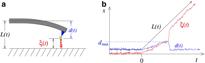
Dynamic force spectroscopy (DFS) setup and measurement. (a) Schematic of a DFS pulling experiment. A pulling device with spring constant K and reference control position L(t) is attached to one end of a bond. As the device is lifted, it deflects by amount d, but also stretches the observed bond coordinate ξ, which is a measurement of the underlying true bond coordinate x. (b) Schematic of trajectories for L(t), d(t), and ξ(t) ≡ L(t) − d(t). In reconstructions based on rupture forces, the maximum value d_max determines the force at rupture, indicated by the sharp increase in ξ(t). To see this figure in color, go online.

While such approaches allow reconstruction of simple parametric forms of the bond potential, they require careful tuning of experimental parameters. For example, the pulling device cannot be too stiff if a transient barrier and rupturing behavior is desired (32). Moreover, event-based reconstruction requires pulling over a range of carefully tuned speeds. Most importantly, reconstruction based on rupture forces also ignores the full wealth of information contained in measurements of the individual displacements, and is at best ill conditioned (33).

Indeed, there exists extensive literature on drift recovery for random walks using trajectory measurements and/or relating energy gaps to work averages over paths using work theorems (14,15,34–36). In fact, the diffusivity cannot be independently extracted using work-theorem-based reconstructions. Nonetheless, spatial variations in diffusivity are intertwined with displacement trajectory-based recovery of the underlying bond potential. Variations in diffusivity are associated with varying landscape roughness (37), which ultimately arises from projections of higher-dimensional trajectories onto the path defined by the external pulling (38). Thus, spatially varying diffusivity contains information on how a high-dimensional system projects down to form a one-dimensional potential profile.

Regardless of inversion method, samples of Brownian trajectories are taken pointwise, meaning that the recovery of continuous functions governing Brownian motion is ill posed. Inference on random walks is typically performed at a certain spatial resolution wherein averaging of observations occurs (39–42). Computationally, these approaches typically involve discretization of the solution domain (39,40,42), where piecewise-constant solutions are obtained through binwise Bayesian inference, maximum likelihood, or moment-matching as in the case of work theorems (15,43,44).

Bayesian path integral-based approaches have been developed for the recovery of mathematically continuous solutions, where candidate reconstructions are weighted by properties encoded in a distribution that reflects a priori knowledge. In this vein, Lemm et al. (45) demonstrated such an approach for the recovery of potential functions from paths observed in quantum systems. Similar methodology has been adapted to the problem of unsupervised density estimation (46,47).

We will show that using this type of approach in the DFS setting naturally incorporates the simultaneous reconstruction of both diffusivity and bond potential. Bayesian theory then provides a procedure for inference, uncertainty quantification, and parameter identification. The application of Bayesian theory in this way also defines the inverse problem in its more-natural continuum representation using partial differential equations. Any discretization used in solving the partial differential equations is independent of the problem formulation.

Here, we develop a path integral-based empirical Bayesian procedure to reconstruct bond forces and diffusivities directly from trajectory measurements. Our method is general in that we need make no assumption about the pulling protocol or device spring constant; the only assumption made is applicability of the one-dimensional Brownian motion. We provide an efficient numerical procedure, test our approach on simulated trajectories, and show that very reasonable numbers of trajectories are sufficient to simultaneously reconstruct complicated multiminima bond potentials and diffusivities. The sensitivity of bond-force reconstruction to the diffusivity profile is also explored and a physical interpretation of our regularization discussed.

Materials and Methods

Problem setup

Fig. 1 shows a schematic of DFS in which a bond is pulled apart along the spatial direction x, while the bond displacement ξ(t) is measured and recorded. We assume that the bond coordinate is an overdamped random variable obeying the Smoluchowski equation. As derived in Sancho et al. (48), adiabatic elimination of the inertial variable through application of the fluctuation-dissipation theorem results in a stochastic differential equation of the form

$$\text{d}\xi =A\left(\xi ,t\right)\text{d}t+\sqrt{2D\left(\xi \right)}\text{d}W,$$ (1)

where W is a Wiener process, D(x) is the space-dependent diffusivity function, and A(x,t) is the spatially varying drift. Because D(x) is assumed to be spatially varying, the exact form of A(x,t) is to be chosen according to the stochastic integration scheme used. If one uses Stratonovich rules for integrating Eq. 1, the appropriate convective drift is A(x,t) ≡ −D(x)∂_xΦ(x,t), where Φ(x,t) is the combined molecular and device potential. The expected overdamped Fokker-Planck equation (FPE) for the probability distribution function P(x,t) takes the form (44) of

$$\frac{\partial P\left(x,t\right)}{\partial t}-\frac{\partial }{\partial x}\left(PD\left(x\right)\frac{\partial \Phi }{\partial x}\right)=\frac{\partial }{\partial x}\left(D\left(x\right)\frac{\partial P}{\partial x}\right).$$ (2)

If, however, one wishes to use Itô calculus to evaluate Eq. 1, one finds that the appropriate form for the drift is A(x,t) ≡ −D(x)∂_xΦ(x,t) + ∂_xD(x). The motion described by this drift term results from forces arising from a potential gradient and a diffusivity gradient. The additional drift force arises from a statistical bias in the motion induced by a spatially varying diffusivity. Applying Itô calculus to Eq. 1 and using this definition of A(x,t) yields the same overdamped FPE (44). Either choice of A(x,t) yields the correct Stratonovich physics (49) and Eq. 2 as long as the correct integration rule is followed in each case. In this article, for ease of implementing stochastic simulations, we use A(x,t) ≡ −D(x)∂_xΦ(x,t) + ∂_xD(x) and the Itô calculus to evaluate Eq. 1.

The total dimensionless (normalized by k_BT) potential Φ(x,t) is composed of the molecular bond potential U(x) and a moving harmonic potential arising from the pulling device (typically an optical trap or atomic force microscopy cantilever, as shown in Fig. 1). The origin L(t) of the harmonic potential is controlled by the pulling device. Together, the total potential takes the form

$$\Phi \left(x,t\right)=\underset{\text{bond}}{\underbrace{U\left(x\right)}}+\underset{\text{harmonic}}{\underbrace{\frac{K}{2}{\left(x-L\left(t\right)\right)}^2}},$$ (3)

where K is the device spring constant. After differentiating Eq. 3, one finds

$$A\left(x,t\right)=D\left(x\right)\left[F\left(x\right)+\stackrel{F_a}{\overbrace{K\left(L\left(t\right)-x\right)}}\right]+D^{\prime }\left(x\right),$$ (4)

where F(x) = −dU(x)/dx is the intermolecular bond force, and F_a is the force applied by the pulling apparatus. In practice, the pulling device is moved at a constant velocity V starting from an initial position L₀: L(t) = L₀ + V_t. Equation 4 shows that pulling (increasing L(t)) increases the drift thereby encouraging displacement of the bond coordinate away from x = L₀. The goal of such experiments is to infer properties of the bond potential U(x), from many realizations of ξ(t).

The bond force F(x) will be assumed to be a smooth continuous function that will be decomposed in the form

$$F\left(x\right)=F_d\left(x\right)+f\left(x\right),$$ (5)

where F_d(x) = κx^−ν (κ ≥ 0, ν > 1) is the most divergent component of the force associated with the divergent part of the potential U(x) ∼ x^−ν (ν > 1) as x → 0. At large separations, we assume the total force vanishes and f(x → ∞) → 0. The behavior of F near x = 0 is not particularly interesting, so we will make the simplifying assumption that F_d(x) = 6(x/2)⁻⁷, and restrict our recovery problem to the region [L₀, ∞). Ultimately, our reconstruction for the potential and diffusivity for x > L₀ will not be too sensitive to the exact form of the divergence; there will be very few trajectories that sample the strongly repulsive region where x is small. The smooth function f(x) captures all other features of the intermolecular bond force we wish to reconstruct. We impose vanishing boundary conditions at x = 0 and x → ∞, but do not assume f(x) obeys any particular parametric form. In our subsequent inverse problem, because F_d(x) is specified, and molecular forces are conservative, the reconstruction of f(x) will be equivalent to reconstruction of F(x) and, up to an additive constant, the molecular potential U(x).

Empirical Bayes formulation

Because the recovery of continuous f(x) directly from discretely sampled data is ill posed, we now describe a path-integral-based Bayesian interpretation of the so-called Tikhonov regularization (45–47,50–55). The key feature this method is the usage of a smoothness penalty to select solutions from particular well-behaved function spaces. The choice of function space and smoothing is considered prior knowledge and is determined either from physical considerations or estimated directly from the data. The inverse problem is then investigated through the evaluation of a partition function, using a path integral over the given function space. A general form of Tikhonov regularization manifests itself through a prior probability density on f(x) of the form

$$\pi \left(f|\mathit{\theta }\right)={\mathcal{Z}}_f^{-1}\text{exp}\left\{-\frac{1}{2}{\int }_0^{\infty }f\left(y\right)R_f\left(-\Delta \right)f\left(y\right)\text{d}y\right\},$$ (6)

where Δ is the Laplacian operator, R_f is a self-adjoint pseudo-differential regularization operator containing some parameters θ, and $\mathcal{Z}$_f is a normalization factor. We assume for now that we know R_f, R_g, and their associated parameters θ. A more thorough discussion on their choice is presented in the next section.

To enforce the positivity of D(x), we express diffusivity in terms of the log-diffusivity

$$g\left(y\right)=\text{log}\frac{D\left(y\right)}{D_0},$$ (7)

where D₀ > 0, a uniform background diffusivity, can be estimated directly from the data (see Eqs. S15 and S16 given in the Supporting Material). We assume a similar prior distribution on the log-diffusivity g(y) of the form

$$\pi \left(g|\mathit{\theta }\right)={\mathcal{Z}}_g^{-1}\text{exp}\left\{-\frac{1}{2}{\int }_0^{\infty }g\left(y\right)R_g\left(-\Delta \right)g\left(y\right)\text{d}y\right\}.$$ (8)

The normalization factors $\mathcal{Z}$_f, $\mathcal{Z}$_g do not affect the inference of f(x) and g(x), but are important when one wishes to self-consistently determine specific forms of regularization R_f, R_g. Equations 6 and 8 enforce that the prior probability distributions are over a collection of functions f(x) and g(x) that have Gaussian spatial autocorrelations. These autocorrelations are determined by the Green’s functions of the pseudo-differential-operators R_f and R_g, which can be thought of as kernels encoding certain magnitude and scale information about the spatial variability in the set of functions f and g.

Experimentally, a trajectory is composed of measurements of bond displacements, ξ ≡ (ξ₁,ξ₂,…,ξ_N), taken at times t₁,t₂,…,t_N. If the force F(x) = F_d(x) + f(x) and diffusivity D(x) = D₀e^g(x) are given, the likelihood or probability of observing a given trajectory ξ_j (0 ≤ j ≤ N) can be formulated in terms of the product of transition probabilities $\pi \left(\mathit{\xi }|f,g\right)={\prod }_j\text{Pr}\left({\xi }_{j+1}|{\xi }_j,f,g\right)$. In the limit as δt → 0, the transition probabilities, interpreted using Itô rules, are themselves Gaussian with mean A(ξ_j,t_j)δt and variance 2D(ξ_j)δt (see Eq. S11 and the Supporting Methods in the Supporting Material for the derivation). We have assumed that measurement times t_i and displacements ξ_i are precisely measured (the error remains small relative to 2Dδt), and that the sampling frequency is sufficiently high (δt = t_j+1 – t_j is small).

Given a collection of M independently measured trajectories X = {ξ^(α)}, (1 ≤ α ≤ M), one can integrate the stochastic differential equation (Eq. 1) using A(x,t) ≡ −D(x)∂_xΦ(x,t) + ∂_xD(x) and the Itô calculus to find the total likelihood function for observing the entire ensemble of trajectories as a product of the likelihoods of the individual trajectories:

$$\begin{array}{c}\pi \left(\mathbf{X}|f,g\right)=\prod _{\alpha }\pi \left({\mathit{\xi }}^{\left(\alpha \right)}|f,g\right)\\ =\text{exp}\left\{-\sum _{\alpha ,j}\left[\frac{{\left({\xi }_{j+1}^{\left(\alpha \right)}-{\xi }_j^{\left(\alpha \right)}-A\left({\xi }_j^{\left(\alpha \right)},t_j\right)\delta t\right)}^2}{4D\left({\xi }_j^{\left(\alpha \right)}\right)\delta t}\right]\right\}\times \prod _{\alpha ,j}\sqrt{\frac{1}{4\pi D\left({\xi }_j^{\left(\alpha \right)}\right)\delta t}}.\end{array}$$ (9)

We remind the reader here that Eq. 9 is invariant to the choice of stochastic calculus as long as the right choice of A(x,t) is used. Using Bayes’ rule, the posterior probability distribution for f and g, given observation of X and regularization parameters θ, is

$$\pi \left(f,g|\mathbf{X},\mathit{\theta }\right)=\frac{\pi \left(\mathbf{X}|f,g\right)\pi \left(f|\mathit{\theta }\right)\pi \left(g|\mathit{\theta }\right)}{\pi \left(\mathbf{X}\right)}\equiv \frac{e^{-H\left[f,g|\mathbf{X},\mathit{\theta }\right]}}{\mathcal{Z}},$$ (10)

where $\mathcal{Z}$ is a dimensionless normalization constant and H is an information Hamiltonian given by

$$H\left[f,g|\mathbf{X},\mathit{\theta }\right]=\frac{1}{2}{\int }_0^{\infty }f\left(y\right)R_f\left(-\Delta \right)f\left(y\right)dy+\frac{1}{2}{\int }_0^{\infty }g\left(y\right)R_g\left(-\Delta \right)g\left(y\right)\text{d}y+\frac{1}{2}\sum _{\alpha ,j}\text{log}D\left({\xi }_j^{\left(\alpha \right)}\right)+\sum _{\alpha ,j}\frac{{\left({\xi }_{j+1}^{\left(\alpha \right)}-{\xi }_j^{\left(\alpha \right)}-A\left({\xi }_j^{\left(\alpha \right)},t_j\right)\delta t\right)}^2}{4D\left({\xi }_j^{\left(\alpha \right)}\right)\delta t},$$ (11)

where the last two terms arise from taking the logarithm of the likelihood given in Eq. 9. As a reminder, we have assumed that measurement noise is negligible relative to the inherent stochastic noise of the Brownian motion at timescale δt. Relaxation of this assumption would require the evaluation of an additional path-integral in ξ, as performed in Masson et al. (39,56).

Recall that the terms f and g are present implicitly in the drift term of the Hamiltonian, as defined in Eq. 4. The most-probable reconstructions for f(x), g(x), minimize Eq. 11. These reconstructions constitute the maximum a posteriori solution, or the specific choice of force F(x) = F_d(x) + f(x) and diffusivity D(x) = D₀e^g(x) that minimizes Eq. 11. They are found by solving the coupled system of Euler-Lagrange equations

$$\begin{array}{l}\frac{\delta H}{\delta f}=0\text{and}\hfill \\ \frac{\delta H}{\delta g}=0,\hfill \end{array}$$ (12)

and constitute the mean-field or classical solution. The main difficulty in solving these equations lies in inverting a large matrix of rank equal to the number of observed trajectory positions. A computational method for approximating the solution about evaluation points is presented in the Supporting Methods in the Supporting Material. In this method, sufficient statistics of the data are computed only a single time, after which optimization occurs in a lower-dimensional space. Furthermore, the sufficient statistics are independent of the regularization parameters, allowing an arbitrary number of candidate solutions to be computed without reprocessing the data. While the resulting optimization problem is nonconvex, we discuss three reasonable choices for the initialization state in Supporting Methods section 4 c in the Supporting Material. Through analysis of a related scalar problem, we also note that the Hamiltonian is locally convex over most of the admissible function space.

Regularization parameters and uncertainty quantification

Up to this point, we have assumed that one knows what to use for the operators R_f(−Δ) and R_g(−Δ). Because these operators can be thought of as prior information, their choice can be motivated from physical considerations whenever such information is available (50). Typically, the uncertainty in the reconstructed functions arises from the mathematical ill-posedness of the inverse problem. However, in the DFS problem, the one-dimensional bond potential is a projection from a high-dimensional macromolecular stochastic process and the effective bond potential will suffer physical thermal fluctuations that also contribute to its uncertainty. Therefore, it is desirable to choose R_f, R_g directly from the data, which may shed light on how orthogonal modes are thermally coupled to the one-dimensional bond potential.

Note that if R_f = R_g = 1 is chosen as the regularization operator, the corresponding Green’s function is the Dirac δ-distribution. This situation corresponds to the spatially unregularized inverse problem. Numerically, if this inverse problem is solved over a discrete lattice, then the solution is the recovery of piecewise constant force and diffusivity. For a more physically realistic and better-behaved inversion, it is convenient to restrict R_f, R_g to a family of operators that impose spatial regularity.

Henceforth, we will assume f and g are infinitely differentiable and use operators of the form

$$\begin{array}{l}{R}_f\left(-\Delta \right)=\frac{e^{-{\gamma }_f\Delta /2}}{{\beta }_f\sqrt{2\pi {\gamma }_f}},\hfill \\ R_g\left(-\Delta \right)=\frac{e^{-{\gamma }_g\Delta /2}}{{\beta }_g\sqrt{2\pi {\gamma }_g}}.\hfill \end{array}$$ (13)

Using the operators in Eq. 13, one need only determine two parameters for each field: the spatial scale γ and the reciprocal temperature β. Assuming that no information is known about these parameters, one may utilize any number of available information-theory-based methods, such as Bayesian model comparison or maximum marginal likelihood (empirical Bayes). Here, we describe the application of approximate maximum marginal likelihood to the problem of choosing regularization parameters.

As its name implies, maximum marginal likelihood estimation seeks to determine unknown parameters θ = (β_f, β_g, γ_f, γ_f) by maximizing the marginal likelihood function

$$\pi \left(\mathbf{X}|\mathit{\theta }\right)=\iint \mathcal{D}f\mathcal{D}g\pi \left(\mathbf{X}|f,g\right)\pi \left(f|\mathit{\theta }\right)\pi \left(g|\mathit{\theta }\right)$$ (14)

with respect to θ. This expression can be interpreted as the probability of obtaining the observed data given the regularization parameters θ. The optimization of this quantity requires the evaluation of the path integrals with respect to both fields f and g. These integrals can be approximated using the semiclassical approximation (50) in which the Hamiltonian (Eq. 11) is expanded about its extremal points f^∗, g^∗ to quadratic order:

$$H\left[f,g|\mathbf{X},\mathit{\theta }\right]\approx H\left[f^{\ast },g^{\ast }|\mathbf{X},\mathit{\theta }\right]+\frac{1}{2}\iint \mathit{\phi }{\left(y\right)}^t{\mathbf{\Sigma }}^{-1}\mathit{\phi }\left(z\right)\text{d}y\text{d}z.$$ (15)

The difference of the functions from their classical solution is defined by the new field

$$\mathit{\phi }\left(x\right)=\left[\begin{array}{c}f\left(x\right)-f^{\ast }\left(x\right)\\ g\left(x\right)-g^{\ast }\left(x\right)\end{array}\right],$$

and the semiclassical Hessian Σ⁻¹ matrix is

$${\mathbf{\Sigma }}^{-1}={\left[\begin{array}{cc}\frac{{\delta }^{2}H}{\delta f\left(y\right)\delta f\left(z\right)}& \frac{{\delta }^{2}H}{\delta f\left(y\right)\delta g\left(z\right)}\\ \frac{{\delta }^{2}H}{\delta g\left(y\right)\delta f\left(z\right)}& \frac{{\delta }^{2}H}{\delta g\left(y\right)\delta g\left(z\right)}\end{array}\right]}_{f^{\ast },g^{\ast }}.$$ (16)

The probability distribution over the functions f(x) and g(x) has a spread defined by $\mathbf{\Sigma }$, which encodes the distribution of f(x) and g(x) about their most likely values f^∗(x) and g^∗(x), thereby providing an estimate of the errors in the estimates f^∗(x) and g^∗(x). Performing the resulting Gaussian path integral ${\mathcal{Z}}_f^{-1}{\mathcal{Z}}_g^{-1}\int \mathcal{D}\mathit{\phi }{e}^{-H\left[\mathit{\phi }|\mathbf{X},\mathit{\theta }\right]}$ yields the semiclassical approximation to the negative of the marginal likelihood function

$$-\text{log}\pi \left(\mathbf{X}|\mathit{\theta }\right)=\text{const}+H\left[f^{\ast },g^{\ast }|\mathbf{X},\mathit{\theta }\right]+\text{Tr}\text{log}\mathbf{\Sigma }-\text{Tr}\text{log}{G}_f\left(x,y\right)-\text{Tr}\text{log}{G}_g\left(x,y\right),$$ (17)

where the additive constant is independent of the regularization parameters and the TrlogG_f and TrlogG_g terms come from the normalization terms $\mathcal{Z}$_f and $\mathcal{Z}$_g. Note that an implicit θ-dependence arises in all terms involving R_f, R_g, and the data-derived f^∗ and g^∗. In the Supporting Methods in the Supporting Material, we show that the computation of Eq. 17 is equivalent to the computation of the eigenvalues of a finite-dimensional matrix—allowing for quick evaluation of Eq. 17 for use in standard optimization routines.

Reconstruction procedure

Summarizing, our general procedure for simultaneous force and diffusivity reconstruction is:

• 1)If unknown, estimate the background diffusivity D₀ and the spring constant K directly from data using Eqs. S15 and S16 in the Supporting Material.
• 2)
  For each choice of regularization parameters β_f,g, γ_f,g:

  • a)
    Solve for the maximum a posteriori solution f^∗, g^∗ by solving Eqs. 12 using the method outlined in Supporting Methods in the Supporting Material.
  • b)
    Compute the semiclassical variance matrix Σ by inverting the matrix in Eq. 16.
• 3)Choose regularization parameters that minimize Eq. 17.

Results

To demonstrate our method, we first simulated data from DFS pulling experiments using two different bond potentials and diffusivities. Fig. 2 shows representative examples of simulated trajectories. Although the dynamics are governed by complicated bond potentials and spatially varying diffusivities, individual trajectories are rather featureless. The distributions that solve the associated FPE are also qualitatively generic and featureless. However, data across multiple trajectories can be aggregated as shown on the right of Fig. 2.

Figure 2.

Trajectory data. Simulations using bond force and diffusivity given by (a) Eqs. S1 and S2 in the Supporting Material and (b) Eq. S3 in the Supporting Material. (Solid) Three individual simulated trajectories (out of 10³). Each trajectory represented a different pulling experiment of duration 5 s, sampled at 10 kHz, with V = 20, K = 0.15. (Shaded region) Compactly supported area; it represents the intensity of all 10³ trajectories through each space-time point. While these trajectories are rather featureless, the histogram of positions observed across all trajectories (up to time 5 s) is shown on the right and contains more features. Each point in the histogram represents a single instance in which a position is sampled. Thus, each trajectory can sample a specific position many times. The total number of sample points is 10³ trajectories × 10 kHz × 5 s = 5 × 10⁷. These data can be aggregated across different experimental conditions and contain sufficient information with which to simultaneously reconstruct f(x) and g(x). To see this figure in color, go online.

Next, discrete measurements were extracted from our simulated trajectories and used within our inference scheme to recover the bond force and diffusivities that were used to generate the simulated data in the first place. We implemented our inference method in the software language Python 2.7.5 (https://www.python.org/) using the SciPy 0.14.0 library (http://www.scipy.org/) for numerical optimization. (The source code for our implementation is publicly available at https://github.com/joshchang/dfsinference.) In all of the following examples, functions were recovered within the interval from ∼x = 4 to x = 32, where L₀ = 4 was assumed to be the starting point for the bond coordinate. In this interval, 200 evenly spaced evaluation points were chosen.

Fig. 3 shows reconstruction from trajectories simulated under dynamics determined by two examples of the pair of functions (F(x), D(x)). These functions are explicitly given by Eqs. S1–S3 in the Supporting Material. The bond force shown in Fig. 3 corresponds to the F(x) and D(x) used to generate the trajectories shown in Fig. 2. Although D(x) is spatially varying, we first use a constant $D_0^{\ast }$ obtained from Eq. S16 in the Supporting Material in our reconstruction. Note that regularized reconstruction (blue, dashed curves) results in smoother and more stable recovery of F(x) = F_d(x) + f(x) compared to unregularized recovery (thin, red curves). However, regardless of regularization, neglecting the true spatial dependence of D(x) results in poor reconstruction of the true bond force.

Figure 3.

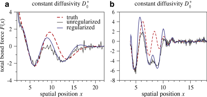
Failure to account for diffusivity variations. Molecular bond force F^∗(x) = f^∗(x) + F_d(x) derived from unregularized (thin black) and regularized (solid blue) reconstruction data simulated using a given ground truth force field (dashed red). For reconstruction purposes, a constant diffusivity $D_0^{\ast }$ estimated from Eq. S16 in the Supporting Material was assumed. Although regularization allows for smoother and more stable reconstructions, the neglect of spatial structure in D(x) leads to inaccurate results. For example, the reconstructions in (a) cannot accurately determine the position of the minima, while those in (b) miss the minima entirely. The errors are especially apparent in regions where the diffusivity is significantly different from the constant value: (a) $D_0^{\ast }$ = 1.0042, (b) $D_0^{\ast }$ = 0.9995. To see this figure in color, go online.

Fig. 4 demonstrates regularized reconstruction where diffusivity variations are taken into account. It also shows how reconstructions change as the number of observed trajectories increases. Uncertainty quantification is also provided, where the ∼95% posterior credible interval is shown by the yellow-shaded region. Using physically reasonable values, we see that a reasonable number of experiments (∼10² − 10³) is sufficient for simultaneous recovery of D(x) and complicated potentials.

Figure 4.

Regularized reconstruction with a variable number of trajectories. Reconstruction of the bond force and diffusivity is given in Eq. S3 in the Supporting Material. (Shaded yellow) 95% semiclassical posterior confidence interval. (Gray) Unregularized binwise reconstruction. The noising reconstruction here arises from narrow bins and intrinsic sampling variability. (Blue) Regularized reconstructions. Optimal parameters used at trajectories were $D_0^{\ast }$ = 0.9995, β_f = 19,884, β_f = 2.28, and γ_g = 1.02. To see this figure in color, go online.

Discussion

We have developed a nonparametric Bayesian approach to the simultaneous reconstruction of spatially varying bond force and diffusivity functions directly from stochastic displacement trajectories measured in DFS experiments. Our approach introduces both a path integral with explicit data terms in the energy and a Tikhonov regularization term in the form of a prior distribution over the functions to be recovered. As only weak regularity conditions based on the notion of L² integrability are used, the method is flexible in the range of functions that can be recovered. Moreover, the regularization provides a formal basis for uncertainty quantification of the reconstructed functions. The approach presented here is versatile in that it is nonparametric, allows a broad class of functions to be stably reconstructed, is based on the statistically optimal principle of Bayesian inference, and can allow aggregation of data sets from experiments performed under different conditions (such as pulling speed V, device spring constant K, and temperature).

Our method directly uses the inherently stochastic nature of bond trajectories to provide a likelihood formulation for use in Bayesian inference. Hence, we are able to simultaneously and self-consistently reconstruct two functions: the bond force and the diffusivity. In our example recoveries of Fig. 3, spatially varying diffusivity is not included, and qualitatively incorrect reconstruction of the bond force arises. Potentials reconstructed using constant diffusivity can yield minima in the wrong position or miss them altogether. To the best of our knowledge, prior methods for extracting information from DFS experiments, including those that exploit work theorems (14,15,34,44), are not able to reconstruct diffusivity profiles. For this reason, they provide an incomplete picture of the bond dynamics.

Simultaneous bond potential and diffusivity reconstruction provides added insight into the molecular physics of the bond. Although our test data are generated by simulations using a fixed, static ground truth molecular potential U(x) and bond force F(x) = −dU(x)/dx, real molecules contain many coupled degrees of freedom. The effective potential along the direction of bond pulling is a potential of mean force (PMF). Coupling of bond displacements to other modes of the molecule collectively contributes to a transverse restoring force, creating a confined molecular tunnel that varies in thickness. Such a picture of the high-dimensional potential naturally leads to axial variations in diffusivity (37,38). Even though our simulations were generated from a fixed PMF U(x), real data are derived from pulling bonds that are subject to temporal fluctuations from thermal coupling to other modes of the molecule. Thus, both axially varying diffusivity and thermal fluctuations are naturally subsumed in our reconstruction of both F(x) and D(x) from real data.

Our approach further complements those using work theorems because approaches using statistics of work data can be used to recover only the mean-field solution f^∗(x). Moreover, our approach also does not rely on an initial equilibrium distribution. The regularization operator, determined from data, incorporates the inherent uncertainty arising from the ill-posedness of the static inverse problem as well as the physical thermal fluctuations of the function to be reconstructed. As the amount of data increases (i.e., if more experimental trajectories are collected), the posterior distribution for f and g will reflect more of the physical uncertainty arising from the thermal fluctuations. Our empirically determined regularization, along with the spatially varying channel diffusivity representation of the high-dimensional molecular bond, provides a picture that complements the notion of a one-dimensional PMF.

Another feature of our methodology is the inclusion of uncertainty quantification, which provides a handle for optimizing pulling protocols and improving recoveries. When full trajectories are observed and sampled, one has access to displacements in a vicinity about any particular spatial location x. The reconstruction of the functions at x utilizes trajectory measurements observed in the neighborhood of that location, weighted by distance relative to a characteristic length-scale $\sqrt{\gamma }$ (see Eq. S86 in the Supporting Material). Typically, $\sqrt{\gamma }$ spans more than one local data bin, and self-consistent reconstructions using significantly less experimental data are possible. Theoretically, the recovery error of the bond force is a function of the number of locally observed displacements, the local diffusivity, and the net drift (see Eq. S86 in the Supporting Material). In particular, the error is at a minimum when the net drift is zero, or when the pulling force is equal and opposite to the intrinsic bond force.

In Fig. 4, we empirically investigated the recovery error as a function of the number of pulling trajectories performed. These plots demonstrate that features of the two functions can already be seen with a single trajectory, are qualitatively similar to the ground truth at 100 trajectories, and are quantitatively accurate at 1000 trajectories. Examining Fig. 4 in the context of Fig. 2, one sees that spatial regions that are more heavily sampled are recovered with fewer pulling experiments. By directly observing trajectories ξ, one may extract information content after a few pulls to determine optimal adjustments in K and V. For example, K and V can be modified to better probe undersampled regions of the spatial coordinate, and data from experiments using different parameters can be aggregated and used toward the final reconstruction.

A key assumption of our method is smoothness of the underlying functions f and g that describe the bond motion. This assumption could be relaxed by exploring regularization in other L^p spaces, for 0 < p ≤ 1. The conceptual challenge lies in formulating an analog to the Gaussian measure that is present for separable inner product spaces. This mathematical hurdle is a significant barrier to the development of a Bayesian theory over such function spaces.

In this article, we have used the regularization operator guaranteeing infinite differentiability of the reconstructions. If infinite differentiability is not desired, other choices are possible (50). We note, however, that the commonly used Laplacian (−Δ) operator is not appropriate because its corresponding Green’s function in $\mathbb{R}$¹ does not have the correct decay characteristics that one would expect of the bond force.

The knowledge that diffusivity is pointwise nonnegative is an example of prior knowledge. We chose to enforce this constraint by expressing the diffusivity as the exponential of an analytical function g. This choice had the additional benefit of making the Hamiltonian smooth in g. It is notable that other choices for satisfying this constraint may have benefits—for instance the use of D = |g|². Future modifications of this work could explore alternative parameterizations of the diffusivity such as this one.

Ideally, one chooses regularization to represent one’s prior knowledge of the functions. For instance, one may know that the functions should have no variations below a certain spatial scale. In practice, this type of knowledge may not be available. We have utilized an empirical Bayesian approach, thereby using the data to estimate the regularization parameters. Reconstruction given the optimal parameters within the empirical Bayesian approach is shown by the blue curves in Fig. 4. Our work can be extended to a full Bayesian treatment through use of priors on these parameters—albeit at higher computational cost. Another simple extension of this work is the case of nonnegligible observation noise, by approximation of an additional path integral as in Masson et al. (39,56).

The ease of simultaneous reconstruction of F(x) and D(x) also suggests that our analysis can be extended to reconstruct potential landscapes in a few higher dimensions (15,57), such as those arising in catch bonds (58,59). Our approach can be readily adapted to reconstructing energy and internal mobility profiles in extended biopolymers and multimolecular assemblies that exhibit complicated multiminimum energy and diffusivity profiles (11,19,60,61).

Author Contributions

T.C. posed the inverse problem; P.-W.F. performed simulations of the DFS experiment; J.C.C. developed the statistical method and analytical approximations; J.C.C. developed the numerical approximation method and implemented the method; J.C.C. and T.C. drafted the article; and all authors were involved in editing the article.

Editor: Sean Sun.

References

- 1.Arridge S.R. Optical tomography in medical imaging. Inverse Probl. 1999;15:R41. [Google Scholar]
- 2.Coleman T.F., Li Y., Verma A. Reconstructing the unknown local volatility function. J. Comput. Finance. 1999;2:77–102. [Google Scholar]
- 3.Renò R. Nonparametric estimation of the diffusion coefficient of stochastic volatility models. Econom. Theory. 2008;24:1174–1206. [Google Scholar]
- 4.Evans E., Ritchie K., Merkel R. Sensitive force technique to probe molecular adhesion and structural linkages at biological interfaces. Biophys. J. 1995;68:2580–2587. doi: 10.1016/S0006-3495(95)80441-8. [DOI] [PMC free article] [PubMed] [Google Scholar]
- 5.Heymann B., Grubmüller H. Dynamic force spectroscopy of molecular adhesion bonds. Phys. Rev. Lett. 2000;84:6126–6129. doi: 10.1103/PhysRevLett.84.6126. [DOI] [PubMed] [Google Scholar]
- 6.Merkel R., Nassoy P., Evans E. Energy landscapes of receptor-ligand bonds explored with dynamic force spectroscopy. Nature. 1999;397:50–53. doi: 10.1038/16219. [DOI] [PubMed] [Google Scholar]
- 7.Neuman K.C., Nagy A. Single-molecule force spectroscopy: optical tweezers, magnetic tweezers and atomic force microscopy. Nat. Methods. 2008;5:491–505. doi: 10.1038/nmeth.1218. [DOI] [PMC free article] [PubMed] [Google Scholar]
- 8.Lang M.J., Fordyce P.M., Block S.M. Simultaneous, coincident optical trapping and single-molecule fluorescence. Nat. Methods. 2004;1:133–139. doi: 10.1038/nmeth714. [DOI] [PMC free article] [PubMed] [Google Scholar]
- 9.Hinterdorfer P., Dufrêne Y.F. Detection and localization of single molecular recognition events using atomic force microscopy. Nat. Methods. 2006;3:347–355. doi: 10.1038/nmeth871. [DOI] [PubMed] [Google Scholar]
- 10.Rawicz W., Smith B.A., Evans E. Elasticity, strength, and water permeability of bilayers that contain raft microdomain-forming lipids. Biophys. J. 2008;94:4725–4736. doi: 10.1529/biophysj.107.121731. [DOI] [PMC free article] [PubMed] [Google Scholar]
- 11.Koch S.J., Wang M.D. Dynamic force spectroscopy of protein-DNA interactions by unzipping DNA. Phys. Rev. Lett. 2003;91:028103. doi: 10.1103/PhysRevLett.91.028103. [DOI] [PubMed] [Google Scholar]
- 12.Jobst M.A., Schoeler C., Nash M.A. Investigating receptor-ligand systems of the cellulosome with AFM-based single-molecule force spectroscopy. J. Vis. Exp. 2013;82:e50950. doi: 10.3791/50950. [DOI] [PMC free article] [PubMed] [Google Scholar]
- 13.Maitra A., Arya G. Model accounting for the effects of pulling-device stiffness in the analyses of single-molecule force measurements. Phys. Rev. Lett. 2010;104:108301. doi: 10.1103/PhysRevLett.104.108301. [DOI] [PubMed] [Google Scholar]
- 14.Hummer G., Szabo A. Free energy reconstruction from nonequilibrium single-molecule pulling experiments. Proc. Natl. Acad. Sci. USA. 2001;98:3658–3661. doi: 10.1073/pnas.071034098. [DOI] [PMC free article] [PubMed] [Google Scholar]
- 15.Hummer G., Szabo A. Free energy profiles from single-molecule pulling experiments. Proc. Natl. Acad. Sci. USA. 2010;107:21441–21446. doi: 10.1073/pnas.1015661107. [DOI] [PMC free article] [PubMed] [Google Scholar]
- 16.Rief M., Oesterhelt F., Gaub H.E. Single molecule force spectroscopy on polysaccharides by atomic force microscopy. Science. 1997;275:1295–1297. doi: 10.1126/science.275.5304.1295. [DOI] [PubMed] [Google Scholar]
- 17.Puchner E.M., Gaub H.E. Force and function: probing proteins with AFM-based force spectroscopy. Curr. Opin. Struct. Biol. 2009;19:605–614. doi: 10.1016/j.sbi.2009.09.005. [DOI] [PubMed] [Google Scholar]
- 18.Fernandez J.M., Li H. Force-clamp spectroscopy monitors the folding trajectory of a single protein. Science. 2004;303:1674–1678. doi: 10.1126/science.1092497. [DOI] [PubMed] [Google Scholar]
- 19.Dobrovolskaia I.V., Arya G. Dynamics of forced nucleosome unraveling and role of nonuniform histone-DNA interactions. Biophys. J. 2012;103:989–998. doi: 10.1016/j.bpj.2012.07.043. [DOI] [PMC free article] [PubMed] [Google Scholar]
- 20.Ros R., Eckel R., Anselmetti D. Single molecule force spectroscopy on ligand-DNA complexes: from molecular binding mechanisms to biosensor applications. J. Biotechnol. 2004;112:5–12. doi: 10.1016/j.jbiotec.2004.04.029. [DOI] [PubMed] [Google Scholar]
- 21.Rief M., Pascual J., Gaub H.E. Single molecule force spectroscopy of spectrin repeats: low unfolding forces in helix bundles. J. Mol. Biol. 1999;286:553–561. doi: 10.1006/jmbi.1998.2466. [DOI] [PubMed] [Google Scholar]
- 22.Clausen-Schaumann H., Seitz M., Gaub H.E. Force spectroscopy with single bio-molecules. Curr. Opin. Chem. Biol. 2000;4:524–530. doi: 10.1016/s1367-5931(00)00126-5. [DOI] [PubMed] [Google Scholar]
- 23.Helenius J., Heisenberg C.-P., Muller D.J. Single-cell force spectroscopy. J. Cell Sci. 2008;121:1785–1791. doi: 10.1242/jcs.030999. [DOI] [PubMed] [Google Scholar]
- 24.Anselmetti D., Hansmeier N., Toensing K. Analysis of subcellular surface structure, function and dynamics. Anal. Bioanal. Chem. 2007;387:83–89. doi: 10.1007/s00216-006-0789-3. [DOI] [PubMed] [Google Scholar]
- 25.Benoit M., Gabriel D., Gaub H.E. Discrete interactions in cell adhesion measured by single-molecule force spectroscopy. Nat. Cell Biol. 2000;2:313–317. doi: 10.1038/35014000. [DOI] [PubMed] [Google Scholar]
- 26.Evans E.A., Calderwood D.A. Forces and bond dynamics in cell adhesion. Science. 2007;316:1148–1153. doi: 10.1126/science.1137592. [DOI] [PubMed] [Google Scholar]
- 27.Dudko O.K., Hummer G., Szabo A. Theory, analysis, and interpretation of single-molecule force spectroscopy experiments. Proc. Natl. Acad. Sci. USA. 2008;105:15755–15760. doi: 10.1073/pnas.0806085105. [DOI] [PMC free article] [PubMed] [Google Scholar]
- 28.Dudko O.K. Single-molecule mechanics: new insights from the escape-over-a-barrier problem. Proc. Natl. Acad. Sci. USA. 2009;106:8795–8796. doi: 10.1073/pnas.0904156106. [DOI] [PMC free article] [PubMed] [Google Scholar]
- 29.Freund L.B. Characterizing the resistance generated by a molecular bond as it is forcibly separated. Proc. Natl. Acad. Sci. USA. 2009;106:8818–8823. doi: 10.1073/pnas.0903003106. [DOI] [PMC free article] [PubMed] [Google Scholar]
- 30.Fuhrmann A., Anselmetti D., Reimann P. Refined procedure of evaluating experimental single-molecule force spectroscopy data. Phys. Rev. E Stat. Nonlin. Soft Matter Phys. 2008;77:031912. doi: 10.1103/PhysRevE.77.031912. [DOI] [PubMed] [Google Scholar]
- 31.Evstigneev M., Reimann P. Dynamic force spectroscopy: optimized data analysis. Phys. Rev. E Stat. Nonlin. Soft Matter Phys. 2003;68:045103. doi: 10.1103/PhysRevE.68.045103. [DOI] [PubMed] [Google Scholar]
- 32.Shapiro B.E., Qian H. A quantitative analysis of single protein-ligand complex separation with the atomic force microscope. Biophys. Chem. 1997;67:211–219. doi: 10.1016/s0301-4622(97)00045-8. [DOI] [PubMed] [Google Scholar]
- 33.Fok P.-W., Chou T. Reconstruction of potential energy profiles from multiple rupture time distributions. Proc. Roy. Soc. A Math. Phys. Eng. Sci. 2010;466:3479–3499. [Google Scholar]
- 34.Hummer G., Szabo A. Free energy surfaces from single-molecule force spectroscopy. Acc. Chem. Res. 2005;38:504–513. doi: 10.1021/ar040148d. [DOI] [PubMed] [Google Scholar]
- 35.Balsera M., Stepaniants S., Schulten K. Reconstructing potential energy functions from simulated force-induced unbinding processes. Biophys. J. 1997;73:1281–1287. doi: 10.1016/S0006-3495(97)78161-X. [DOI] [PMC free article] [PubMed] [Google Scholar]
- 36.Woodside M.T., Block S.M. Reconstructing folding energy landscapes by single-molecule force spectroscopy. Annu. Rev. Biophys. 2014;43:19–39. doi: 10.1146/annurev-biophys-051013-022754. [DOI] [PMC free article] [PubMed] [Google Scholar]
- 37.Zwanzig R. Diffusion in a rough potential. Proc. Natl. Acad. Sci. USA. 1988;85:2029–2030. doi: 10.1073/pnas.85.7.2029. [DOI] [PMC free article] [PubMed] [Google Scholar]
- 38.Best R.B., Hummer G. Coordinate-dependent diffusion in protein folding. Proc. Natl. Acad. Sci. USA. 2010;107:1088–1093. doi: 10.1073/pnas.0910390107. [DOI] [PMC free article] [PubMed] [Google Scholar]
- 39.Masson J.-B., Dionne P., Dahan M. Mapping the energy and diffusion landscapes of membrane proteins at the cell surface using high-density single-molecule imaging and Bayesian inference: application to the multiscale dynamics of glycine receptors in the neuronal membrane. Biophys. J. 2014;106:74–83. doi: 10.1016/j.bpj.2013.10.027. [DOI] [PMC free article] [PubMed] [Google Scholar]
- 40.Türkcan S., Alexandrou A., Masson J.-B. A Bayesian inference scheme to extract diffusivity and potential fields from confined single-molecule trajectories. Biophys. J. 2012;102:2288–2298. doi: 10.1016/j.bpj.2012.01.063. [DOI] [PMC free article] [PubMed] [Google Scholar]
- 41.Schuss Z. Vol 170. Springer; New York: 2009. (Theory and Applications of Stochastic Processes: An Analytical Approach, Springer Series on Applied Mathematical Sciences). [Google Scholar]
- 42.Schuss Z. Vol. 180. Springer; New York: 2011. (Nonlinear Filtering and Optimal Phase Tracking, Springer Series on Applied Mathematical Sciences). [Google Scholar]
- 43.Alemany A., Mossa A., Ritort F. Experimental free-energy measurements of kinetic molecular states using fluctuation theorems. Nat. Phys. 2012;8:688–694. [Google Scholar]
- 44.Seifert U. Stochastic thermodynamics, fluctuation theorems and molecular machines. Rep. Prog. Phys. 2012;75:126001. doi: 10.1088/0034-4885/75/12/126001. [DOI] [PubMed] [Google Scholar]
- 45.Lemm J.C., Uhlig J., Weiguny A. Bayesian approach to inverse quantum statistics. Phys. Rev. Lett. 2000;84:2068–2071. doi: 10.1103/PhysRevLett.84.2068. [DOI] [PubMed] [Google Scholar]
- 46.Nemenman I., Bialek W. Occam factors and model independent Bayesian learning of continuous distributions. Phys. Rev. E Stat. Nonlin. Soft Matter Phys. 2002;65:026137. doi: 10.1103/PhysRevE.65.026137. [DOI] [PubMed] [Google Scholar]
- 47.Bialek W., Callan C.G., Strong S.P. Field theories for learning probability distributions. Phys. Rev. Lett. 1996;77:4693–4697. doi: 10.1103/PhysRevLett.77.4693. [DOI] [PubMed] [Google Scholar]
- 48.Sancho J., San Miguel M., Dürr D. Adiabatic elimination for systems of Brownian particles with nonconstant damping coefficients. J. Stat. Phys. 1982;28:291–305. [Google Scholar]
- 49.Ao P., Kwon C., Qian H. On the existence of potential landscape in the evolution of complex systems. Complexity. 2007;12:19–27. [Google Scholar]
- 50.Chang J.C., Savage V.M., Chou T. A path-integral approach to Bayesian inference for inverse problems using the semiclassical approximation. J. Stat. Phys. 2014;157:582–602. [Google Scholar]
- 51.Enßlin T.A., Frommert M., Kitaura F.S. Information field theory for cosmological perturbation reconstruction and nonlinear signal analysis. Phys. Rev. D Part. Fields Gravit. Cosmol. 2009;80:105005. [Google Scholar]
- 52.Cotter S., Dashti M., Stuart A. Bayesian inverse problems for functions and applications to fluid mechanics. Inverse Probl. 2009;25:115008. [Google Scholar]
- 53.Heuett W.J., Miller B.V., 3rd, Periwal V. Bayesian functional integral method for inferring continuous data from discrete measurements. Biophys. J. 2012;102:399–406. doi: 10.1016/j.bpj.2011.12.046. [DOI] [PMC free article] [PubMed] [Google Scholar]
- 54.Farmer C. Algorithms for Approximation. Springer; Heidelberg, Germany: 2007. Bayesian field theory applied to scattered data interpolation and inverse problems; pp. 147–166. [Google Scholar]
- 55.Stuart A. Inverse problems: a Bayesian perspective. Acta Numer. 2010;19:451–559. [Google Scholar]
- 56.Masson J.-B., Casanova D., Alexandrou A. Inferring maps of forces inside cell membrane microdomains. Phys. Rev. Lett. 2009;102:048103. doi: 10.1103/PhysRevLett.102.048103. [DOI] [PubMed] [Google Scholar]
- 57.Suzuki Y., Dudko O.K. Single-molecule rupture dynamics on multidimensional landscapes. Phys. Rev. Lett. 2010;104:048101. doi: 10.1103/PhysRevLett.104.048101. [DOI] [PubMed] [Google Scholar]
- 58.Marshall B.T., Long M., Zhu C. Direct observation of catch bonds involving cell-adhesion molecules. Nature. 2003;423:190–193. doi: 10.1038/nature01605. [DOI] [PubMed] [Google Scholar]
- 59.Pereverzev Y.V., Prezhdo O.V., Sokurenko E.V. Distinctive features of the biological catch bond in the jump-ramp force regime predicted by the two-pathway model. Phys. Rev. E Stat. Nonlin. Soft Matter Phys. 2005;72:010903. doi: 10.1103/PhysRevE.72.010903. [DOI] [PubMed] [Google Scholar]
- 60.Hinczewski M., Gebhardt J.C.M., Thirumalai D. From mechanical folding trajectories to intrinsic energy landscapes of biopolymers. Proc. Natl. Acad. Sci. USA. 2013;110:4500–4505. doi: 10.1073/pnas.1214051110. [DOI] [PMC free article] [PubMed] [Google Scholar]
- 61.Rico F., Gonzalez L., Scheuring S. High-speed force spectroscopy unfolds titin at the velocity of molecular dynamics simulations. Science. 2013;342:741–743. doi: 10.1126/science.1239764. [DOI] [PubMed] [Google Scholar]
Associated Data
This section collects any data citations, data availability statements, or supplementary materials included in this article.