Strategic parenting, birth order, and school performance

Abstract

Fueled by new evidence, there has been renewed interest about the effects of birth order on human capital accumulation. The underlying causal mechanisms for such effects remain unsettled. We consider a model in which parents impose more stringent disciplinary environments in response to their earlier-born children’s poor performance in school in order to deter such outcomes for their later-born offspring. We provide robust empirical evidence that school performance of children in the National Longitudinal Study Children (NLSY-C) declines with birth order as does the stringency of their parents’ disciplinary restrictions. When asked how they will respond if a child brought home bad grades, parents state that they would be less likely to punish their later-born children. Taken together, these patterns are consistent with a reputation model of strategic parenting.

1 Introduction

Interest on the effects of birth order on human capital accumulation has been reinvigorated by several recent studies (Black et al. 2005; Conley and Glauber 2006; Gary-Bobo et al. 2006) which present new empirical evidence of birth order effects. For example, Black et al. (2005) (BDS, hereafter) find large and robust effects of birth order on educational attainment. However, despite the convincing results, the underlying causal mechanisms generating such findings remain unsettled and researchers remain quite limited in their ability to distinguish between alternative birth order theories. The literature on birth order effects documents declining patterns of completed education and earnings across birth order. To the extent that we care about those outcomes, it might be of interest to understand the source of these birth order effects. If, for some reasons, parents engage in different parenting strategies with children of different birth order, these children will perform while in school, and this could be one of the reasons why they eventually go on to complete more education and have higher earnings.

In thinking about children’s behavior, it is important to remember that parents can resort to a variety of mechanisms to influence it. In particular, they can limit or grant access to important sources of utility for children. This paper advances an hypothesis that has not been previously considered in the generating process for birth order effects in educational outcomes: We consider differential parental disciplining schemes arising from the dynamics of a parental reputation mechanism. One channel that can generate birth order effects is characterized by Hao et al. (2008) (HHJ, hereafter). A key insight of their paper is that birth order effects arise endogenously as the result of viewing parent-child interactions as a reputation game in which parents “play tough” when their older children engage in bad behavior—tougher than caring or altruistic parents would prefer—in an attempt to establish a reputation of toughness to deter bad behavior amongst their younger children. Thus, we hypothesize that one mechanism that gives rise to birth order effects is this form of strategic parenting and responses by their children implied by game-theoretic models of reputation in repeated games.

While the focus of HHJ was teenage risky behavior, their insight that the incentives for strategic parenting will vary across the birth order of parents’ offspring can be applied in other contexts. In the context of this paper, we will think of parents developing a reputation for strict parenting practices with their first born children in the hope of inducing (paternalistic) preferred school effort levels among their later-born offspring. We first document striking patterns of school performance across birth order as children transit from late childhood into early adolescence. We do so by exploiting maternal perceptions of her children’s performance elicited from the female respondents in National Longitudinal Survey of Youth, 1979. We then go on to explore whether similar parental reputation dynamics as those advanced by HHJ are present in our context using different parenting measures and a different sample. Unlike the single shot outcomes explored by HHJ, school performance is observed multiple periods and thus provides parents with multiple opportunities to respond to their children’s actions. Our context therefore provides even greater opportunities for parents to invest in reputation and influence their children’s school performance.

While our focus is on assessing the evidence concerning this type of strategic parenting, there are certainly other reasons why one could observe birth order effects in school performance. In Section 2, we review the alternative theories of the effects of birth order on various behaviors, including educational outcomes. The analysis undertaken in this paper is not intended to refute these theories; rather, in many cases, we think our hypothesis about the role of strategic parenting in birth order effects is complementary with many of these other theories. However, throughout the paper, we present evidence which shows that these other theories cannot account for all of the birth order patterns we find. We also examine several potential threats to the validity of our estimates. We find very robust evidence of birth order effects in measures of school performance that is consistent with children responding to the strategic use of parental monitoring and discipline. While our ability to link these parenting practices to the specific instances of school performance is limited by our data, as noted above, we make use of parents’ reported parenting intentions, namely what parents say they would do in response to their children getting bad grades in school. Based on this measure, we find parents engaging in strategic parenting practices by birth order. The use of these parental intentions data is, we think, a new and promising strategy for mitigating the inherent endogeneity problems that plague the inferences one can draw from the relationship between children’s observed behaviors and observed parental responses to them.

The paper proceeds as follows. As already noted, Section 2 reviews the relevant literature and alternative theories of the effects of birth order on various behaviors, including educational outcomes. Section 3 describes the data we use in our analysis, namely that on the children of female respondents in the National Longitudinal Survey of Youth, 1979. In Section 4, we present estimates of the effects of birth order on measures of children’s performance in school and examine several potential threats to the validity of our estimates. In Section 5, we examine differences in parental monitoring and discipline of their children by birth order. Therein, we present evidence on the link between observed parenting practices and the school performance of their children as well as a measure of parents’ intentions of how they would to the hypothetical situation of their children getting bad grades in school. In Section 6, we offer some concluding observations of the findings in this paper.

2 Review of the birth order literature

In this section, we briefly review the literature on birth order effects and on the links between the effort of students in school and their academic performance and achievement.

There is a substantial literature on birth order effects in education. Zajonc (1976), Olneck and Bills (1979), Blake (1981), Hauser and Sewell (1985), Behrman and Taubman (1986), and Kessler (1991), among others, found mixed results that provide support for a variety of birth order theories ranging from the “no-one-to-teach” hypothesis to the theory of differential genetic endowments. However, with the strong birth order effects found in Behrman and Taubman (1986) and, more recently, in Black et al. (2005) and Booth and Kee (2009), the literature seems to be settling in favor of the existence of such effects and moving towards consideration and sophisticated testing of alternative mechanisms to account for such effects. For example, Price (2008) provides empirical support in time-use data for a modern version of the “dilution hypothesis,” namely that for at least a limited time, the first born does not have to share the available stock of parental quality time input with other siblings, whereas those born later usually enjoy more limited parental input as parents are not able to match the increased demand for their “quality time.”¹

In another strand of research, mostly in psychology, the issue of birth order effects in IQ has been examined. In particular, Rodgers et al. (2000, 2001) have consistently sided against the existence of such a relationship and they have criticized studies for confounding “within-family” and “between-family” processes and by attributing to the former, patterns that are actually shaped by the latter.² More recently, Black et al. (2007) and Bjerkedal et al. (2007) find strong and significant effects of birth order on IQ within families in a large data set from Norway, but Whichman et al. (2006) insist, using a multilevel approach, that the effects only arise between families and they disappear within the family. The debate remains open as Zajonc and Sulloway (2007) criticize Whichman et al. (2006) on several grounds and reach the opposite conclusion. Finally, Whichman et al. (2007) address the issues raised by Zajonc and Sulloway (2007) and confirm their previous findings.

There is also a sizable literature on the links between students’ effort in school and their academic performance (see, for example, Natriello and McDill 1986; Wolters 1999; Covington 2000; Stinebrickner and Stinebrickner 2008). There appears to be a fairly clear consensus in this literature that greater student effort improves academic performance. For example, Stinebrickner and Stinebrickner (2008) show the importance of actual school effort on school performance, but our understanding of the factors that lead to greater student effort and how such effort interacts with other features of a student’s home and school environments are less clear. Relevant to this paper, there is a literature on the relationship between parenting and parental involvement and student effort and, ultimately, performance (see Trautwein and Koller 2003; Fan and Chen 2001; Hoover-Dempsey 2001). Most studies in this literature do not model or account for the endogenous nature of how the amount of school effort exerted by children is affected by parental incentives and policy instruments.

An exception to this shortcoming of the literature is a recent paper by De Fraja et al. (2010). These authors develop an equilibrium model in which parents, schools, and students interact to influence the effort of students and their performance and test this model using data from the British National Child Development Study. At the same time, De Fraja et al. (2010) do not characterize the potential informational problems that parents have in monitoring their children’s input and the potential role of strategic behavior on the part of parents in attempting to influence the children’s effort. Our paper attempts to fill this deficit in the literature.

2.1 Alternative theories of birth order effects

There are several alternative causal hypotheses in the literature trying to explain the relationship between birth order and schooling. First, there could be parental time dilution noted above. Under this hypothesis, the earlier-born siblings enjoy more parental time than later-born siblings. This may explain why earlier borns do better in school. Second, there could be differences in the genetic endowment of children by birth order. Indeed, later-born siblings are born to older mothers, so they are more likely to receive a lower quality genetic endowment. Third, first borns and parents’ experience with them may have undue influence on parents’ subsequent fertility decisions. According to this theory, a “bad draw,” e.g., a difficult-to-raise, problematic child, may cause parents to curtail their subsequent fertility whereas an easy-to-rear first-born would not. More generally, this phenomenon implies selection in the quality of parents’ last-born child, with it being of lower quality than the average. Fourth, closely related to the “confluence model” of Zajonc, the “no-one-to-teach” hypothesis postulates that the last born will not benefit from teaching a younger sibling. Without this pedagogic experience, the last born will not develop strong learning skills. Fifth, it may well be possible that the later-born siblings are more affected by changes in family structure, e.g., divorce, since later-born children are more likely to spend more of their lives exposed to such family disruptions.³ Last, but not least, first borns may enjoy higher parental investment for insurance purposes or simply because parents are more likely to enjoy utility from observing their eventual success in life.

While all the above theories predict that earlier-born siblings will do better, it is worth noting that it is possible that the effect can go in the other direction. For example, parents might learn to teach better. In this case, parents commit mistakes with those born earlier, but they are more proficient, experienced parents when the later-born siblings need to be raised. It also can be the case that, if there are financial constraints, the later-born siblings might be raised at times in which parental resources are more abundant. However, as we document below, the predictions of these two theories run counter to our findings. If financial resources or parenting experience are important to explain school performance, we would expect the later-born siblings to be the ones who particularly benefit from them. However, our results point out that it is the earlier born who do better. While this does not mean these hypotheses are invalid, it certainly suggests that, on net, their quantitative significance is not that large relative to that of other theories.

While acknowledging the merits of these alternative theories and evidence in the previous literature concerning their legitimacy, below, we advance a novel, complementary mechanism that can induce birth order effects in school performance. It highlights the role of incentives faced by children to perform well in school as well as the reputation concerns of lenient parents.

2.2 Parental reputation and child school performance

As noted in Section 1, we draw on the game-theoretic literature on reputation models. Such models were initially developed in the industrial organization literature in response to the chain store paradox of Selten (1978). In particular, Kreps and Wilson (1982) and Milgrom and Roberts (1982) developed models in which the introduction of a small amount of incomplete information gives rise to a different, more intuitive type of equilibrium. HHJ pioneered the use of this type of models in a family context to analyze teenage risk-taking behavior.

Consider a finite-horizon game between parents and children being played in families with more than one child. In particular, the typical family has a total of N children. Consider a long-lived player (the parent or parents) facing a new short-lived player (the child) at each round of the game. In any round t, t = 1, …, N, the parents and the child of that round observe the entire history of play between the parent and the older children. In particular, the younger siblings observe the choices made by their N − t older siblings and the punishment decisions of their parents when older siblings performed poorly in school. Parents can be of one of two types. They may be “tough parents,” i.e., the commitment type that will always punish a child’s poor performance in school, or parents are “lenient,” i.e., the type of parents that dislike punishing their children and would only do so for strategic considerations. In the first round of the game, played with the oldest child, the parents’ type is not known by that child or her younger siblings. Let ${\widehat{\mu }}^1$ denote the children’s belief or probability that their parents are of the tough type and $1-{\widehat{\mu }}^1$ that they are lenient. At each round of the game, t, t > 1, the younger siblings will update their beliefs in a Bayesian fashion based on the accumulated information about the school performance of older children and how their parents responded to these performances. Denote this updated belief, or probability, that the parent is a tough type as ${\widehat{\mu }}^t$. Note that if older siblings always do well in school, then the younger siblings will not have had the occasion to observe whether their parents punish or accommodate poor performance in school and, as a result, will have no basis for updating their prior beliefs, i.e., ${\widehat{\mu }}^t={\widehat{\mu }}^1$.

It can be shown that a sequential equilibrium for this finitely repeated game exists (see Kreps and Wilson 1982, or Milgrom and Roberts, 1982). The defining event in this reputation game is the observation of some parental leniency in response to poor school performance at some round t, i.e., at some birth order t. If parents reveal themselves to be of the lenient type by not punishing the poor school performance of one of their children, ${\widehat{\mu }}^t$ drops to zero and remains there until the end of the game. From then on, the children will fear no punishment from their revealed-to-be-lenient parent whose threats are no longer credible.

The equilibrium of this reputation game between parents and their children is characterized by two phases. In the first phase, played in the early rounds of the game between parents and their earlier-born children, uncertainty about parental type and threat of punishment induces these children to exert high levels of effort in school to deliver good school performance and prevent the triggering of potential punishments coded in the parenting rule. In this phase, bad grades will translate into loss of privileges anyway. If a parent is tough, he will punish by principle. If the parent is a lenient type, she will still punish poor performance in order to establish and/or maintain a reputation for toughness so as to prevent later-born children from taking advantage of her leniency. As a result, we expect earlier-born children playing mostly through this initial phase of the equilibrium to do better in school.⁴ As the rounds of the game proceed, the number of remaining children at risk to play the game declines. At some point, the reputation benefits of punishment for a lenient parent are less than the disutility of witnessing their child’s suffering autonomy loss. Depending on how small ${\widehat{\mu }}^1$ is and how few rounds in the game remain, i.e., how many remaining children a parent has, it will be likely for some of these children to “test the waters” by exerting low school effort and exploring what happens in response. After the first parental accommodating behavior is observed for a lenient parent, the second phase of the game is triggered in which later-born siblings do not put effort in school and go unpunished (note that a tough parent type will choose to punish poor performance for each of their children and never accommodate such behavior). If lenient parents are more prevalent in the population, there is greater uncertainty about parental type in the initial rounds that ends up extracting more effort and better performance from children who play in those initial rounds.

The model delivers some predictions that can be taken directly to the data. In particular, earlier-born siblings are predicted to put more effort in school and should end up performing better. Moreover, parents are more likely to establish rules of behavior with the earlier-born, engage in a more systematic monitoring of earlier-born’s schoolwork, and increase supervision in the event of low school performance. Below, we provide evidence on the validity of these predictions for children’s performance in school and parental responses to it by birth order.

3 The data

We exploit data from the children of female respondents of the National Longitudinal Survey of Youth, 1979 (NLSY79). These data (NLSY-C) contain information on all of the children born to women in the NLSY79, so we potentially observe all of their children as they transition between the ages of 10 and 14, the focus of our analysis. Crucially, many of these women have two or more children, so we are able to directly explore birth order effects that arise in these families.

TV watching and, more recently, video gaming and social networking are time-intensive activities that usually crowd out, at least partially, the time that could be used for homework or study. Indeed, there exists a vast literature in psychology documenting the detrimental effects of TV watching on school performance. Therefore, these activities are natural places to look for parental discipline schemes. Children value these activities highly and parents may be able to enforce and monitor restrictions on their access.

Useful for our purposes, the NLSY-C includes some detailed information on parenting. Some questions ask the mother and/or the children about different features about the parent-child relationship. We also exploit other parenting rules as reported by the children and/or the mother. Crucially, we are able to observe multiple self-reports from the same mother about all of her kids, and we observe those at two and sometimes three points in time. We restrict the analysis to children between the ages of 10 and 14.⁵ However, having repeated observations of parenting rules applied to each child over time allows us to identify changing parenting strategies across birth order by comparing siblings of different birth order once they transition across a given common age.

On the other hand, the NLSY-C does not have systematic information on grades except for a specific supplemental school survey fielded in 1995–1996 about school years 1994–1995. However, the NLSY-C includes a self-report about how the mother thinks each of her children is doing in school. The specific question is: “Is your child one of the best students in class, above the middle, in the middle, below the middle, or near the bottom of the class?” Useful for our purposes, the same questions are asked of the mother separately for each child and in several waves. Note that even when these self-reports could be validated against school transcripts, it can be argued that it is the parental subjective belief about the child’s performance what really matters at the end. We do, however, validate the mother’s perceptions below, exploiting limited transcript data from the 1995–1996 School Supplement.

4 Birth order effects in perceptions of school performance

In this section, we provide evidence from our data concerning differences by birth order in the academic performance of the children of the NLSY79 data. Table 1 and Fig. 1 show that there exists a clear association between school performance (as perceived by the mother) and birth order. Since the NLSY-C has very few observations coming from families with more than four siblings, we focus our analysis on families with 2, 3, or 4 children. The table shows that while 34 % of first born children are considered “one of the best in the class,” only 27 % of those coming fourth in the birth order reach such recognition. On the other hand, only 7.3 % of first borns are considered “below the middle or at the bottom of the class,” while 11.7 % of fourth borns are classified in such manner by their mothers.

Table 1.

Mother’s evaluation of child’s academic standing by birth order

	Birth order (%)
	1st	2nd	3rd	4th
One of the best students in the class	33.8	31.8	29.0	27.2
Above the middle	25.1	24.3	23.6	22.5
In the middle	33.8	35.7	38.3	38.5
Below the middle	5.5	6.2	7.0	8.1
Near the bottom of the class	1.8	2.0	2.1	3.6

Children of the NLSY, 1990–2008. Maternal reports elicited about each of her children

Fig. 1.

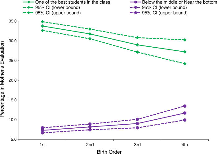
Birth order and perceptions of school performance

One possible concern with the results in Table 1 is that they may confound birth order and family size effects, an issue that has been recognized very early in the development of the birth order literature. Figure 2 explores birth order effects within families of specific sizes. Higher birth orders, by construction, belong in families of bigger size. As pointed out by Behrman and Taubman (1986), such families locate themselves at a different locus of the quantity-quality tradeoff. Therefore, we risk attributing to birth order what really comes from family size. As can be seen in the figure, birth order effects appear to persist in all these families, regardless of size.⁶

Fig. 2.

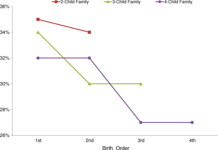
Birth order, family size, and percent of children perceived to be at top of their class

A second concern with the results in Table 1 is that they show clear evidence of inflation in perceived school performance, i.e., maternal assessments appear to show a mother’s Lake Wobegon effect about their own children. However, this need not be a problem as long as the sign and magnitude of these misperceptions do not vary with birth order. In Table 2, we validate maternal perceptions. Higher GPAs of children obtained in the School Supplement are associated with significantly lower chances of being perceived to be at the bottom of the class and significantly higher chances to be classified as one of the best students in the class. Re-estimating the same models including birth order measures shows that “misperceptions”—the differences between perceived and actual performance—are not correlated with birth order. Therefore, to the extent that mothers are too optimistic about their own children performance, but they are so for all of their own children, we account for this mother-specific bias when we include family-fixed effects in our models of perceived school performance.

Table 2.

Validating mother’s perception of child’s school performance

	Ordered probit		Probit		LPM
	Linear (1)	Non-parametric (2)	Linear (3)	Non-parametric (4)	Linear (5)	Non-parametric (6)
GPA	−0.499a (0.092)		0.188a (0.041)		0.168a (0.034)
GPA = 2		−0.902a (0.257)		0.357b (0.177)		0.191b (0.082)
GPA = 3		−0.976a (0.259)		0.423a (0.158)		0.266a (0.079)
GPA = 4		−1.870a (0.304)		0.678a (0.119)		0.557a (0.101)
Birth order	0.063 (0.114)	0.074 (0.119)	−0.062 (0.054)	−0.065 (0.055)	−0.043 (0.046)	−0.051 (0.047)
Mean dep var		0.33	0.33	0.33	0.33
Observations	180	180	180	180	180	180

Robust standard errors in parentheses. Ordered probit uses 1 = top, 2 = above middle, 3 = middle, 4 = below middle, 5 = bottom. The probit and linear probability models (LPM) use 1 = best, 0 = otherwise (the LPM is estimated using ordinary least squares). Controls include age and gender. In non-parametric specifications, GPA = 1 is the omitted category

^asignificant at 1 %

^bsignificant at 5 %

More formally, we follow Black et al. (2005) and explore birth order effects in academic performance by estimating the following two linear models for the probability that the child i in family h is being considered by his/her mother to be one of the best students in the class in year t. The first specification we consider imposes linearity across birth orders

$${\text{BestStudent}}_{\mathit{iht}}={\mathrm{NYS}}_{\mathit{iht}}+X_{\mathit{iht}}^{\prime }\beta +{\mathrm{\lambda }}_h+{\mathrm{\lambda }}_t+{\epsilon }_{\mathit{iht}}$$ (1)

where BestStudent_iht is equal to 1 if child i in family h who in year t was rated by their parents as one of the best students in their class and X_iht includes controls for child’s age and gender (and family size when pooling all families). NYS_i is the number of younger siblings, a measure of birth order that imposes linearity. The λ_ts denote survey year effects and the λ_hs denote family-fixed effects.

Our second specification is more non-parametric in the sense that it allows different effects for different birth orders.

$${\text{BestStudent}}_{\mathit{iht}}={\displaystyle \sum _{k=2}^4{\alpha }_k{\text{BirthOrder}}_{\mathit{kih}}+X_{\mathit{iht}}^{\prime }\beta +{\mathrm{\lambda }}_h+{\mathrm{\lambda }}_t+{\epsilon }_{\mathit{iht}}}$$ (2)

where BirthOrder_kih is a dummy variable that equals 1 when child i is the kth child born in family h and equals 0 otherwise.

Table 3 presents estimates of specifications (1) and (2) for all families and for families with 2, 3, or 4 children respectively. The results in panel A are based on specifications that do not include a family-fixed effect, while those in panel B do. In column 1, the specification imposes linearity of birth order and uses the number of younger siblings as a measure of birth order. In columns 2 through 5, all birth order coefficients are relative to the first born, which is the omitted category. As can be seen in panel A of Table 3, there exist strong birth order effects in all families. The OLS estimates imply that in families of four children, the last child to be born is 15 percentage points less likely to be among the best students in his class. Moreover, when we estimate (1) and (2) controlling for family-fixed effects, the birth order results remain significant and are very similar in sign and magnitude (see panel B of Table 3). Note also that the results in columns 4 and 5 show that the results are not only driven by the last born: We see negative and significant coefficients for children other than the third born in families with three children and the fourth born in families with four children. These results imply that two of the theories described above, “bad draw” and “no-one-to-teach,” cannot be the sole explanation for our findings.

Table 3.

Effect of birth order on mothers’ perceptions of children’s school performance

	All families (1)	All families (2)	2-Child family (3)	3-Child family (4)	4-Child family (5)
Panel A: OLS
Number of younger siblings	0.0517a (0.0070)
2nd Child		−0.0532a (0.0112)	−0.0511a (0.0158)	−0.0618a (0.0189)	−0.0423 (0.0289)
3rd Child		−0.1040a (0.0158)		−0.0869a (0.0227)	−0.1320a (0.0314)
4th Child		−0.1530a (0.0258)		−0.1730a (0.0383)
Female	0.1040a (0.0102)	0.1040a (0.0102)	0.0888a (0.0161)	0.1180a (0.0167)	0.1130a (0.0220)
Mean dep var	0.32	0.32	0.34	0.32	0.30
Panel B: family-fixed effects
Number of younger siblings	0.0529a (0.0113)
2nd Child		−0.0539a (0.0146)	−0.0855a (0.0254)	−0.0496b (0.0232)	−0.0380 (0.0317)
3rd Child		−0.1080a (0.0240)		−0.0632c (0.0346)	−0.1140a (0.0440)
4th Child		−0.1540a (0.0365)		(0.0569)	−0.1510a
Female	0.1110a (0.0113)	0.1110a (0.0113)	0.0937a (0.0194)	0.1240a (0.0178)	0.1200a (0.0217)
Mean dep var observations	0.32 13,194	0.32 13,194	0.34 5607	0.32 5007	0.30 2580

Robust standard errors in parentheses. All of the specifications include a set of year effects and age effects. OLS specifications that pool families of different sizes control for family size effects. Dependent variable equals 1 if child is perceived to be one of the best students in his/her class, equals 0 otherwise

^asignificant at 1 %

^bsignificant at 5 %

^csignificant at 10 %

4.1 Birth order effects in measures of cognitive ability

It is likely that parents would be less likely to punish less capable children for bad grades. If there is a genetic component to performance whereby later children are less capable, we would also see the patterns of school performance that we identify in the data across birth orders. We start observing our children at age 10. Even if there are no genetic differences by birth order, other processes might establish differential levels of cognitive ability by age 10 across birth order within a family. The NLSY79 Child surveys contain a wide range of detailed assessment information about the children of female respondents. Since 1986, a battery of cognitive assessments has been administered biennially for age appropriate children. We use children’s test scores from the three PIAT assessments (math, reading recognition, and reading comprehension) and from the PPVT assessment.

The Peabody Individual Achievement Test (PIAT) is a widely used measure of academic achievement. It consists of three parts. The PIAT math measures a child’s attainment in mathematics. The reading recognition component measures word recognition and pronunciation ability whereas the reading comprehension section measures a child’s ability to understand the meaning of sentences that are read silently. Finally, the Peabody Picture Vocabulary Test (PPVT) measures an individual’s ability to understand American English vocabulary and provides an estimate of scholastic aptitude. The test scores we use are standardized (normed) by age and year. In the NLYS-C, the standardized PIAT scores we use range from 65 to 135, have a mean of 100, and a standard deviation of 15. As can be seen at the bottom of Table 4, these are similar to the mean and standard deviation in our analysis sample. The normed PPVT ranges from 20 to 160.

Table 4.

Effect of birth order on measures of cognitive ability

	PIAT		PIAT reading		PIAT reading
	Math		Recognition		Comprehension		PPVT
	OLS (1)	Family FE (2)	OLS (3)	Family FE (4)	OLS (5)	Family FE (6)	OLS (7)	Family FE (8)
No. of younger siblings	2.351a (0.318)	0.402 (0.586)	2.906a (0.334)	2.058a (0.553)	2.794a (0.298)	2.465a (0.513)	4.061a (0.433)	1.603b (0.727)
3-Children family		−2.910a (0.577)	−3.244a (0.592)		−2.913a (0.537)		−5.265a (0.820)
4-Children family		−6.478a (0.734)	−6.579a (0.769)		−6.167a (0.679)		−11.790a (1.135)
Female	−0.216 (0.446)	−0.910 (0.555)	2.357a (0.448)	2.257a (0.547)	2.054a (0.410)	1.950a (0.521)	−0.276 (0.592)	0.494 (0.672)
Mean dep var	102.3	102.3	105.2	105.2	103.0	103.0	93.98	93.98
Std. dev. dep var	14.02	14.02	14.33	14.33	13.64	13.64	19.75	19.75
Observations	3558	3558	3596	3596	3700	3700	4022	4022

Robust standard errors in parentheses. Specifications include a set of year effects and age effects as well as controls for family size or family-fixed effects. Dependent variables are the standardized scores for each of the assessments. We use the second assessment taken by the child

^asignificant at 1 %

^bsignificant at 5 %

In Table 4, we present estimates for the same model used to produce the results in the previous tables but use the four assessments (3 PIATs and a PPVT) as dependent variables. As can be seen in this table, an early birth order is significantly associated with higher PPVT and two of the PIAT scores. These scores are from the second assessment for these children and capture a permanent measure of cognitive ability for our subsequent analysis. This pattern of birth order effects in cognitive ability could reflect the early operation of reputation dynamics or some of the other mechanisms discussed above. Our findings are consistent with earlier work by Gerner and Lillard (2006) who document birth order effects in cognitive ability.⁷

Having documented the existence of birth order effects in cognitive ability, we now show that our birth order effects in school performance results between the ages of 10 and 14 hold when we control for individual differences in measures of the abilities of children of different birth order within families. Table 5 presents the results for regressions that control for student scores on the PIAT for math, reading recognition, and reading comprehension tests, as well as the PPVT.⁸ As expected, the assessment test scores that proxy for ability all have positive coefficient estimates which are almost always highly significant. Still, birth order has a significant and sizable effect on performance that goes beyond what can be explained through (within family) birth order effects in ability due to some of the theoretical mechanisms discussed earlier.⁹ It should be noted that these results imply that our birth order patterns of school performance cannot be solely due to “differential genetic endowment” or “dilution” theories. If earlier-born siblings are endowed with better genes and this translates into higher cognitive ability, our measures of ability would absorb this and the significance of the birth order variables should dissipate. Similarly, if earlier-born siblings benefited from more quality time in their early childhood, this would be captured in our cognitive ability test scores. The fact that the birth order indicators remain significant indicates that these theories may explain part, but not all, of our birth order findings.

Table 5.

Effect of birth order on mothers’ perceptions of children’s school performance, controlling for child ability

	All families (1)	All families (2)	2-Child family (3)	3-Child family (4)	4-Child family (5)
No. of younger siblings	0.0356a (0.0125)
2nd Child		−0.0341a (0.0155)	−0.0774a (0.0274)	−0.0152 (0.0250)	−0.0260 (0.0333)
3rd Child		−0.0713a (0.0263)		−0.0157 (0.0384)	−0.0912c (0.0469)
4th Child		−0.1080a (0.0414)		−0.1000 (0.0619)
PIAT math	0.0046a (0.0007)	0.0046a (0.0007)	0.0054a (0.0013)	0.0053a (0.0011)	0.0027b (0.0013)
PIAT reading recognition	0.0028a 0.0008)	0.0028a (0.0008)	0.0038b (0.0015)	0.0014 (0.0014)	0.0039a (0.0014)
PIAT reading comprehension	0.0028a (0.0009)	0.0028a (0.0009)	0.0023 (0.0015)	0.0035b (0.0014)	0.0021 (0.0015)
PPVT	0.0024a (0.0005)	0.0024a (0.0005)	0.0032a (0.0009)	0.0023a (0.0008)	0.0014 (0.0011)
Female	0.0997a (0.0123)	0.0997a (0.0123)	0.0972a (0.0212)	0.1070a (0.0194)	0.0975a (0.0234)
Mean dep var	0.330	0.330	0.350	0.330	0.300
Observations	11,354	11,354	4833	4338	2183

Robust standard errors in parentheses. Specifications include a set of year effects and age effects as well as family-fixed effects. Dependent variable equals 1 if child is perceived to be one of the best students in his/her class, equals 0 otherwise

^asignificant at 1 %

^bsignificant at 5 %

^csignificant at 10 %

4.2 Family structure

While family-fixed effects account for time invariant characteristics of the family, they do not account for those characteristics that change over time within families, are correlated with birth order, and that may directly affect children’s school performance. For example, later-born siblings are more likely to be affected by changes in family structure, such as divorce, which can affect the economic and social status of families and the upbringing of children in these households. There is a sizable literature in both sociology and economics that examines the effects of family structure on child outcomes.¹⁰ The NLSY sample provides ample opportunities to control for family structure as a potential determinant of birth order effects. We construct a subsample of “intact” families in which children have not been exposed to any kind of family disruption. This subsample is substantially smaller. We re-estimate our family-fixed effects models for this subsample controlling for child ability. Table 6 presents the results. Despite the substantial loss of power with this sample, birth order still has a significant effect on school performance among intact families. To be clear, we are not claiming that differences in family structure do not affect child outcomes, including a child’s performance in school. Rather, our evidence indicates that the birth order effects that we found in school performance cannot be solely explained by differential exposure to changes in family structure across birth orders.

Table 6.

Effect of birth order on mothers’ perceptions of school performance among intact families

	All families (1)	All families (2)	2-Child family (3)	3-Child family (4)	4-Child family (5)
No. of younger siblings	0.1280a (0.0762)
2nd Child		−0.1510a (0.0774)	−0.2480b (0.106)	0.0222 (0.142)	−0.2280 (0.140)
3rd Child		−0.2450 (0.1590)		0.1660 (0.2460)	−0.5960a (0.3440)
4th Child		−0.3550 (0.2490)			−0.8550 (0.5270)
PIAT math	0.0073b (0.0029)	0.0077c (0.0029)	0.0084b (0.0042)	0.0082 (0.0055)	0.0075 (0.0045)
PIAT reading recognition	0.0022 (0.0030)	0.0020 (0.0031)	−0.0027 (0.0038)	0.0016 (0.0059)	0.0161b (0.0078)
PIAT reading comprehension	0.0037 (0.0030)	0.0040 (0.0031)	0.0054 (0.0047)	0.0056 (0.0059)	−0.0010 (0.0037)
PPVT	0.0034 (0.0021)	0.0033 (0.002)	0.0092c (0.0026)	−0.0013 (0.0023)	−0.0113c (0.0039)
Female	0.0729 (0.0512)	0.0698 (0.0516)	0.1480b (0.0696)	−0.0962 (0.0906)	0.1340 (0.0950)
Mean dep var	0.41	0.41	0.42	0.39	0.45
Observations	173	1173	665	368	140

Robust standard errors in parentheses. Specifications include a set of year effects and age effects as well as family-fixed effects. Dependent variable equals 1 if child is perceived to be one of the best students in his/her class, equals 0 otherwise

^asignificant at 10 %

^bsignificant at 5 %

^csignificant at 1 %

5 Birth order effects in parental rules

In this section, we explore whether birth order effects in performance may arise because of differential parental treatment. We ask whether the data shows any sign of differential parenting by birth order. We provide additional evidence consistent with some of the predictions delivered by the reputation hypothesis and discussed in Section 2.¹¹ In Table 7, we present evidence of the effects of birth order on the existence of parental rules about TV watching. We find strong birth order effects on these rules, and the results are robust to the introduction of family-fixed effects.¹². Earlier-born siblings seem to grow up in a more regulated environment regarding TV relative to their later-born counterparts.

Table 7.

Effect of birth order on existence of parental rules about TV watching

	OLS (1)	OLS (2)	Family FE (3)	Family FE (4)
Number of younger siblings	0.0533a (0.0072)	0.0492a (0.0079)	0.0237b (0.0126)	0.0252b (0.0140)
PIAT math		−0.0009 (0.0006)		−0.0011 (0.0008)
PIAT reading recognition		−0.0014b (0.0007)		−0.0016 (0.0010)
PIAT reading comprehension		0.0005 (0.0007)		0.0001 (0.0010)
PPVT		0.0006 (0.0004)		−0.0009b (0.0005)
Female	−0.0352a (0.0107)	−0.0324a (0.0114)	−0.0260c (0.0125)	−0.0206 (0.0139)
Mean dep var	0.49	0.50	0.49	0.50
Observations	10,982	9894	10,982	9894

Robust standard errors in parentheses. Specifications in columns 1 and 2 include family size effects. Specifications in columns 3 and 4 include family-fixed effects. Dependent variable is equal to 1 if the child reports that there exist rules about watching TV, equals 0 otherwise

^asignificant at 1 %

^bsignificant at 10 %

^csignificant at 5 %

While earlier-born siblings face a more regulated home environment, it is worthwhile to explore whether they actually experience a lack of autonomy to freely choose their preferred time allocation. To address this, we exploit information on reported levels of parental monitoring pressure. In Table 8, we provide evidence of birth order effects in how intensely parents monitor a child’s homework. Consistent with the reputation model, earlier-born siblings face more intense, systematic parental scrutiny regarding homework. Parents are more likely to seek information on how much effort is being exerted by their children on homework. Table 8 shows OLS and family-fixed effects estimates based upon a binary version of the dependent variable which equals 1 when the monitoring is most intense (daily checks on homework).¹³ Indeed, once we control for the measures of ability, the OLS estimate in column 2 of Table 8 shows that each additional younger sibling is associated with an increase of more than two percentage points in the probability of being monitored every day. The effect is 50 % larger once we control for family-fixed effects.¹⁴ An early birth order is clearly associated with a loss of autonomy for the child. A first born child of four-children family is on average approximately 10 percentage points more likely to face daily homework monitoring relative to the last child born in that family.¹⁵

Table 8.

Effect of birth order on intensity of parental monitoring of homework

	OLS (1)	OLS (2)	Family FE (3)	Family FE (4)
No. of younger siblings	0.0120 (0.00814)	0.0218a (0.00880)	0.0385a (0.0167)	0.0318b (0.0184)
PIAT math		−0.0015a (0.0007)		−0.0021a (0.0010)
PIAT reading recognition		−0.0017a (0.0008)		0.0008 (0.0011)
PIAT reading comprehension		0.0006 (0.0008)		−0.0015) (0.0011)
PPVT		−0.0001 (0.0004)		(0.0010) (0.0006)
Female	−0.0404c (0.0117)	−0.0342c (0.0127)	−0.0283b (0.0151)	−0.0212 (0.0167)
Mean dep var	0.43	0.42	0.43	0.42
Observations	8127	7166	8127	7166

Robust standard errors in parentheses. Specifications include a set of year effects and age effects. Specifications in columns 1 and 2 include family size effects. Specifications include a set of year effects and age effects as well as family size effects in columns 1 and 2. Columns 3 and 4 control for family-fixed effects. All specifications control for indicators that measure how often the teacher gives homework. Dependent variable equals 1 if parents check every day on homework, equals 0 otherwise

^asignificant at 5 %

^bsignificant at 10 %

^csignificant at 1 %

While the results in Table 8 are suggestive of reputation dynamics, a sharper implication from parental reputation is that we should expect this loss of autonomy among earlier-born siblings to occur only among those who under-perform in school. In a sense, we should expect to see a significant and positive interaction between our measure of birth order and a measure of under-performance in school. We then consider the following augmented model that features such an interaction:

$${\text{Monitoring}}_{\mathit{iht}}={\alpha }_0+{\alpha }_1{B}_{\mathit{iht}}+{\alpha }_{2}NY{S}_{ih}\times B_{\mathit{iht}}+X_{\mathit{iht}}^{\prime }\beta +{\mathrm{\lambda }}_h+{\mathrm{\lambda }}_t+{\epsilon }_{\mathit{iht}},$$ (3)

where B_ih = 1 if the child is perceived to be under-performing in school.¹⁶ Still, the reputation model predicts that this loss of autonomy would be more likely when the child is not performing well in school. That is, reputation implies α₂ > 0. The results of estimating the augmented model are shown in Table 9. As can be seen in this table, the preferred specification that controls for family-fixed effects and child ability, the estimated interaction effect α₂ is positive, but not significant. While this seems to provide evidence against the reputation model, it is important to notice that our inclusion of B_iht and its interaction with our birth order measure, NYS_ih × B_iht, brings with it endogeneity issues to our modeling of birth order effects in incentives. Indeed, considering in more detail the behavior of the child helps us to understand why these two variables will be likely endogenous, even after controlling for family-fixed effects.

Table 9.

Differential effect of birth order on monitoring intensity among children with bad and good school performance

	OLS (1)	OLS (2)	Family FE (3)	Family FE (4)
B	0.0051 (0.0159)	−0.0136 (0.0176)	0.0176 (0.0198)	0.0050 (0.0215)
B × no. of younger siblings	0.0107 (0.0147)	0.0068 (0.0157)	−0.0037 (0.0173)	0.0046 (0.0186)
No. of younger siblings	0.0088 (0.0099)	0.0190a (0.0105)	0.0402b (0.0174)	0.0307 (0.0190)
PIAT math		−0.0015b (0.0007)		−0.0021b (0.0010)
PIAT reading recognition		−0.0017b (0.0008)		0.0008 (0.0011)
PIAT reading comprehension		0.0006 (0.0008)		−0.0015 (0.0011)
PPVT		−0.0001 (0.0004)		0.0011 (0.0006)
Female	−0.0389c (0.0118)	−0.0350c (0.0127)	−0.0265a (0.0152)	−0.0204 (0.0167)
Mean dep var	0.43	0.42	0.43	0.42
Observations	8127	7166	8127	7166

Robust standard errors in parentheses. Specifications include a set of year effects and age effects as well as family size effects in columns 1 and 2. Columns 3 and 4 control for family-fixed effects. All specifications control for indicators that measure how often the teacher gives homework. Dependent variable equals 1 if child is perceived to be one of the best students in his/her class, equals 0 otherwise. Dependent variable equals 1 if parents check every day on homework, equals 0 otherwise

^asignificant at 10 %

^bsignificant at 5 %

^csignificant at 1 %

The probability that the child under-performs essentially depends on its ability A_i and effort E_i, but how much effort the child allocates to achieve good school performance also depends on the probability of autonomy loss in the event of under-performance. Consider then a linear probability model for under-performance

$$B_{\mathit{iht}}={\theta }_0+{\theta }_1{A}_{\mathit{iht}}+{\theta }_2{E}_{\mathit{iht}}+{\mathrm{\lambda }}_h+{\mathrm{\lambda }}_t+{\eta }_{\mathit{iht}}$$ (4)

where θ₁ < 0 and θ₂ < 0. Now, let effort E_iht depend on ability A_i and the probability of autonomy loss upon bad school performance

$$E_{\mathit{iht}}={\varphi }_0+{\varphi }_1{A}_i+{\theta }_2\mathrm{Pr}(L_{\mathit{iht}}=1|B_{\mathit{iht}}=1)+{\mathrm{\lambda }}_h+{\mathrm{\lambda }}_t+v_{\mathit{iht}}$$ (5)

where L_iht = 1 if the child suffers autonomy loss due to intense parental supervision and monitoring. If we add the parenting equation to this system, we note that NYS_ih × B_iht and B_iht are likely to be endogenous.

$$L_{\mathit{iht}}={\alpha }_0+{\alpha }_1{B}_{\mathit{iht}}+{\alpha }_{2}NY{S}_{ih}\times B_{\mathit{iht}}+X_{\mathit{iht}}^{\prime }\beta +{\mathrm{\lambda }}_h+{\mathrm{\lambda }}_t+{\epsilon }_{\mathit{iht}}$$ (6)

For example, suppose that children observe more than us, the econometricians, about ε_ih, the child i-specific family h unobservables affecting the parental propensity to monitor and supervise at time t. Say ${\epsilon }_{\mathit{iht}}={\epsilon }_{\mathit{iht}}^1+{\epsilon }_{\mathit{iht}}^2$ and children can observe ${\epsilon }_{\mathit{iht}}^1$. We can interpret this as an observable signal (to the child) of parental supervision propensity for that period. The child of course will use this information when forming his beliefs about the probability of losing autonomy in the event of low school performance. Then, we update the effort function to reflect this.

$$E_{\mathit{iht}}={\varphi }_0+{\varphi }_1{A}_i+{\theta }_2\mathrm{Pr}(L_{\mathit{iht}}=1|B_{\mathit{iht}}=1,{\epsilon }_{\mathit{iht}}^1)+{\mathrm{\lambda }}_h+{\mathrm{\lambda }}_t+v_{\mathit{iht}}$$ (7)

It is clear then that high ${\epsilon }_{\mathit{iht}}^1’\mathrm{s}$ will lead to high effort E_iht by increasing the perceived odds of autonomy loss upon bad grades, $\mathrm{Pr}(L_{\mathit{iht}}=1|B_{\mathit{iht}}=1,{\epsilon }_{\mathit{iht}}^1)$. Higher effort will, in turn, translate into higher (i.e., grades a lower probability of observing B_iht = 1), given θ₂ < 0. From our perspective, ε_iht and B_iht will be correlated and will induce bias in our parameter of interest, α₂. Moreover, the estimate will be biased downwards, and therefore, it will prevent us from drawing valid inference regarding the hypothesis that α₂ > 0. As this example shows, parent-child strategic interactions create substantial endogeneity problems in estimating equations that intend to capture important aspects of child and parental behavior.

As is customary in the literature, one could attempt to solve this type of endogeneity problem by relying in some sort of instrumental variable or quasi-experiment Z_iht that should ideally induce exogenous variation in school performance for child i in household h at time t. While finding convincing instruments is usually a difficult task, this is especially difficult in our context, as many potential instruments that do indeed generate random variation in school performance would nevertheless be invalid, as long as they are known by the parent. This is so because those factors, when known by the parents, will be taken into account when executing the parenting strategy. In summary, good instruments are very difficult to find because not only they have to be somewhat random but also need to be unknown by the parents. Parental unawareness of those random factors is especially unlikely because, if they can be verified, children would have incentives to reveal their existence in the hopes of providing attenuating circumstances for bad school performance.

Lacking a good instrument, we pursue an alternative novel approach to test the implications of the reputation model. Consider the probability of intense monitoring given bad grades.

$$\mathrm{Pr}(L_{\mathit{iht}}=1|B_{\mathit{iht}}=1)={\alpha }_0+{\alpha }_1+{\alpha }_{2}NY{S}_{ih}+X_{\mathit{iht}}^{\prime }\beta +{\mathrm{\lambda }}_h+{\mathrm{\lambda }}_t+u_{\mathit{iht}}$$ (8)

where u_iht = E [ε_iht | B_iht = 1]. Note that this specification removes or conditions out the endogenous under-performance measure but still allows us to test for reputation. In a sense, this is a probabilistic model of the parental strategy that integrates out ε_iht. Therefore, if we had access to self-reported probabilities (or likelihood ranges) of monitoring upon bad school performance, we could test for reputation by exploring whether those subjective probabilities vary with birth order. In particular, we would expect a parent’s reported probabilities of increased supervision to be higher for earlier-born siblings.

Fortunately, our data includes such self-reports. The mother was asked about the likelihood that she would take an action (increase the supervision of her child) in response to a hypothetical situation (her child came home with bad grades). That is, we have a measure of the mother’s self-reported likelihood of punishing in a hypothetical situation, rather than her report of what she actually did in response to her child’s actual behavior, where the latter is subject to the above-noted endogeneity. The specific question we exploit in this context is the following:

“If (Child) brought home a report card with grades lower than expected, how likely would you (the mother) be to keep a closer eye on [his/her] activities?”

The following were the allowed responses: not at all likely, somewhat unlikely, not sure how likely, somewhat likely, and very likely. This question was asked, every other year since 1988 to the mother, separately for each child. We work with a dichotomous version of the dependent variable which equals 1 if the mother would be very likely to keep a closer eye on the child in the event of low school performance and zero otherwise. This allows us to easily control for family-fixed effects.¹⁷

This new form of data provides an interesting complement to more standard data on observed behavior because it essentially recovers the parental strategy directly, even in cases in which the child does well in school and never triggers the eventual punishment.

Estimates of the specification in (8) are displayed in Table 10. We find that the more younger siblings a child has, i.e., the lower the birth order, the more likely are parents to report that they would more closely supervise the child in the event of that child bringing home an unexpectedly low performance on a report card. In particular, after controlling for the child’s ability and family-fixed effects, we find that having an additional younger sibling increases the chances that parents report being very likely to increase supervision upon bad school performance by 2.2 percentage points. This implies that within a family with four children, a first born sibling is 6.6 percentage points more likely to have the parent being very likely to punish upon bad grades relative to the last born, i.e., the fourth child in the family.

Table 10.

Effect of birth order on probability that parent would be very likely to increase supervision if child brought on poor report card

	OLS (1)	OLS (2)	Family FE (3)	Family FE (4)
Number of younger siblings	0.0144a (0.0060)	0.0088 (0.0066)	0.0241b (0.0089)	0.0222a (0.0102)
PIAT math		−0.0005 (0.0004)		0.0007 (0.0005)
PIAT reading recognition		0.0001 (0.0005)		−0.0002 (0.0007)
PIAT reading comprehension		0.0011a (0.0006)		−0.0001 (0.0006)
PPVT		0.0001 (0.0003)		−0.0001 (0.0004)
Female	0.0070 (0.0079)	0.0048 (0.0088)	−0.0008 (0.0084)	0.0019 (0.0095)
Mean dep var	0.81	0.81	0.81	0.81
Observations	11,982	10,379	11,982	10,379

Robust standard errors in parentheses. All specifications include a set of year and age variables. Columns 1 and 2 include family size variables, while columns 3 and 4 include family-fixed effects. Dependent variable equals 1 if parents report being very likely to supervise the child more closely in the event of low grades, equals 0 otherwise

^asignificant at 5 %

^bsignificant at 1 %

^csignificant at 10 %

6 Conclusions

A burgeoning literature spanning now more than three decades has documented clear patterns of birth order in educational outcomes and attempted to uncover the underlying mechanism behind them. We contribute to this literature by showing that those born earlier perform better in school. While most of our analysis uses maternal perceptions of school performance, as opposed to true measures of school performance, a validation of perceptions using actual transcript data shows that these findings do no reflect Lake Wobegon effects or, more importantly, any differential misperceptions of performance by birth order. Doing well in school at ages 10–14 can arguably put students at lower risk of dropping out of high school and increase the chances of them eventually attending college. Therefore, we believe our findings have the potential to explain some of the well-documented birth order effects in educational attainment. Our school performance results are robust to controls for family size and even when we examine subsamples of families of a given size.

While we adopt mostly a linear specification to gain efficiency, the results show up also in more non-parametric specifications that allow each birth order to have a different effect in families of different sizes. This non-linear analysis shows that our results are not driven only by first-born or last-born effects. In other words, siblings “in the middle” perform better than last borns, but worse that first borns. More generally, our school performance results are robust to the inclusion of family-fixed effects: Birth order effects arise even when we only exploit within-family variation. We view a child’s school performance at ages 10–14 as being primarily a function of an underlying mostly time-invariant measure of cognitive ability and the effort he/she puts in school. While effort can be manipulated by parenting incentives, the underlying cognitive ability is much less malleable. Since we document similar birth order patterns in measures of cognitive ability, we then show that our school performance results hold even after controlling for these measures. Moreover, the findings also hold in a subsample of intact families, thus minimizing the chance that birth order effects mask differential exposure to family structure disruption that could hinder school performance.

After documenting these novel results, we then provide evidence consistent with parental reputation incentives generating birth order effects in school performance. In particular, we show that earlier-born siblings are more likely to be subject to rules about TV watching and to face more intense parental monitoring regarding homework. We then propose a new reputation test based on parental self-reported likelihood of increased supervision upon bad grades that avoids a potential endogeneity problem that arises when attempting to recover the parenting strategy. We present evidence that mothers are more likely to report that they would increase the supervision of one of their children in the event that child brought home a worse-than-expected report card when the child in question was one of her earlier-born children. While further research is needed to rule out alternative explanations associated with changing cost and technologies of alternative parenting strategies as sibships grow, we believe that results indicate that parental reputation dynamics may explain part of the observed birth order effects in school performance.

References

- Behrman J, Taubman P. Birth order, schooling and earnings. J Labor Econ. 1986;4(3):S121–S145. doi: 10.1086/298124. [DOI] [PubMed] [Google Scholar]
- Bjerkedal T, Kristensen P, Skejeret G, Brevik JI. Intelligence test scores and birth order among young Norwegian men (conscripts) analyzed within and between families. Intelligence. 2007;35(6):503–514. [Google Scholar]
- Black S, Devereux P, Salvanes K. The more the merrier? The effect of family size and birth order on children’s education. Q J Econ. 2005;120(2):669–700. [Google Scholar]
- Black S, Devereux P, Salvanes K. Older and wiser?: birth order and IQ of young men. 2007. (NBER working paper 13237). [Google Scholar]
- Blake J. Family size and the quality of children. Demogr. 1981;18(4):421–442. [PubMed] [Google Scholar]
- Booth AL, Kee HJ. Birth order matters: the effect of family size and birth order on educational attainment. J Popul Econ. 2009;22(2):367–397. [Google Scholar]
- Conley D, Glauber R. Parental education investment and children’s academic risk: estimates of the impact of sibship size and birth order from exogenous variation in fertility. J Hum Resour. 2006;41(4):722–37. [Google Scholar]
- Covington M. Goal theory, motivation and school achievement: an integrative review. Annu Rev Psychol. 2000;51:171–200. doi: 10.1146/annurev.psych.51.1.171. [DOI] [PubMed] [Google Scholar]
- De Fraja G, D’Oliveira T, Zanchi L. Must try harder. Evaluating the role of effort on examination results. Rev Econ Stat. 2010;92(3):577–597. [Google Scholar]
- Ermisch JF, Francesconi M. Family structure and children’s achievements. J Popul Econ. 2001;14(2):249–270. [Google Scholar]
- Fan X, Chen M. Parental involvement and students’ academic achievement: A meta-analysis. Educ Psychol Rev. 2001;13:1–22. [Google Scholar]
- Finlay K, Neumark D. Is marriage always good for children? Evidence from families affected by incarceration. J Hum Resour. 2010;45(4):1046–1088. [Google Scholar]
- Gary-Bobo R, Prieto A, Picard N. Birth-order and sibship sex composition effects in the study of education and earnings. 2006. (Centre for Economic Policy Research Discussion Paper No. 5514). [Google Scholar]
- Gerner J, Lillard D. The effect of birth order on early educational attainment. Cornell University; 2006. (Working paper). [Google Scholar]
- Ginther D, Pollak R. Family structure and children’s educational outcomes: blended families, stylized facts and descriptive regressions. Demogr. 2004;41(4):671–696. doi: 10.1353/dem.2004.0031. [DOI] [PubMed] [Google Scholar]
- Hao L, Hotz VJ, Jin GZ. Games that parents and adolescents play: risky behavior, parental reputation and strategic transfers. Econ J. 2008;118(528):515–555. doi: 10.1111/j.1468-0297.2008.02132.x. [DOI] [PMC free article] [PubMed] [Google Scholar]
- Hauser RM, Sewell WH. Birth order and educational attainment in full sibships. Am Educ Res J. 1985;22(1):1–23. [Google Scholar]
- Hoover-Dempsey KV, Battiato AC, Walker JMT, Reed RP, De-Jong JM, Jones KP. Parental involvement in homework. Educ Psychol. 2001;36:195–209. [Google Scholar]
- Kessler D. Birth order, family size and achievement: family structure and wage determination. J Labor Econ. 1991;9(4):413–426. doi: 10.1086/298275. [DOI] [PubMed] [Google Scholar]
- Kanazawa S. Intelligence, birth order and family size. Pers Soc Psychol Bull. 2012;38:1157–1165. doi: 10.1177/0146167212445911. [DOI] [PubMed] [Google Scholar]
- Kreps D, Wilson R. Reputation and imperfect information. J Econ Theory. 1982;27:253–279. [Google Scholar]
- Lehmann J-YK, Nuevo-Chiquero A, Vidal-Fernandez M. Birth order differences in early inputs and outcomes. IZA Discussion Paper. 2013;(6755) [Google Scholar]
- Lindert P. Sibling position and achievement. J Hum Resour. 1977;12(2):220–241. [Google Scholar]
- McLanahan S, Sandefur G. Growing up with a single parent: what hurts, what helps. Harvard University Press; Cambridge: 1994. [Google Scholar]
- Milgrom P, Roberts J. Predation, reputation and entry deterrence. J Econ Theory. 1982;27:280–312. [Google Scholar]
- Natriello G, McDill E. Performance standards, student effort on homework, and academic achievement. Sociol Educ. 1986;59(1):18–31. [Google Scholar]
- Olneck MR, Bills DB. Family configuration and achievement: effects of birth order and family size in a sample of Brothers. Soc Psychol Rev. 1979;42(2):135–148. [Google Scholar]
- Pavan R. On the production of skills and the birth order effect, working paper. University of London; Royal Holloway: 2013. [Google Scholar]
- Price J. Parent-child quality time: does birth order matter? J Hum Resour. 2008;43(1):240–265. [Google Scholar]
- Rodgers JL, Cleveland HH, van den Oord E, Rowe DC. Resolving the debate over birth order, family size and intelligence. Am Psychol. 2000;55(6):599–510. doi: 10.1037//0003-066x.55.6.599. [DOI] [PubMed] [Google Scholar]
- Rodgers JL, Cleveland HH, van den Oord E, Rowe DC. Birth order and intelligence: together again for the last time? Am Psychol. 2001;56(6–7):523–524. [PubMed] [Google Scholar]
- Selten R. The chain store paradox. Theor Decis. 1978;9:127–159. [Google Scholar]
- Stinebrickner R, Stinebrickner T. The Causal Effect of Studying on Academic Performance. BE J Econ Anal Poli. 2008;8(1) (Frontiers) Article 14. [Google Scholar]
- Tartari M. Divorce and the cognitive achievement of children working paper. University of Chicago; 2014. [Google Scholar]
- Trautwein U, Koller O. The relationship between homework and achievement: still much of a mystery. Educ Psychol Rev. 2003;15:115–45. [Google Scholar]
- Whichman AL, Rodgers JL, McCallum RC. A multi-level approach to the relationship between birth order and intelligence. Pers Soc Psychol Bull. 2006;32(1):117–127. doi: 10.1177/0146167205279581. [DOI] [PubMed] [Google Scholar]
- Whichman AL, Rodgers JL, McCallum RC. Birth order has no effect on intelligence: a reply and extension of previous findings. Pers Soc Psychol Bull. 2007;33(9):1195–1200. doi: 10.1177/0146167207303028. [DOI] [PubMed] [Google Scholar]
- Wolters C. The relation between high school students’ motivational regulation and their use of learning strategies, effort, and classroom performance. Learn Individ Differ. 1999;11(3):281–299. [Google Scholar]
- Zajonc RB. Family configuration and intelligence. Science. 1976;192:227–236. doi: 10.1126/science.192.4236.227. [DOI] [PubMed] [Google Scholar]
- Zajonc RB, Sulloway FJ. The confluence model: birth order as a between family or within family dynamic? Pers Soc Psychol Bull. 2007;33:1187–1194. doi: 10.1177/0146167207303017. [DOI] [PubMed] [Google Scholar]
Associated Data
This section collects any data citations, data availability statements, or supplementary materials included in this article.