

Abstract
Biological membranes exhibit long-range spatial structure in both chemical composition and geometric shape, which gives rise to remarkable physical phenomena and important biological functions. Continuum models that describe these effects play an important role in our understanding of membrane biophysics at large length scales. We review the mathematical framework used to describe both composition and shape degrees of freedom, and present best practices to implement such models in a computer simulation. We discuss in detail two applications of continuum models of cell membranes: the formation of microemulsion and modulated phases, and the effect of membrane-mediated interactions on the assembly of membrane proteins.
1. Introduction
The plasma membrane serves a vital biological role as the cellular boundary. Not only is it the primary barrier that prevents the uncontrolled exchange of material between the cell and its surroundings, it is also instrumental in the spatial organization of cellular components such as the cytoskeleton and proteins embedded in or associated with the membrane. The length scale over which this ordering occurs can be much larger than the size of the molecular components of the membrane, and ranges from tens to hundreds of nanometers.
The principal chemical structure of the plasma membrane is a bilayer of many different types of lipid molecules. While early models considered these lipids as a homogeneous and passive matrix whose main function was to provide an environment in which membrane proteins could exist [1], it has become apparent that the membrane exhibits significant heterogeneities in both lipid and protein composition. In particular, the concept of lipid rafts, domains enriched in sterol- and sphingolipids less than 100 nanometers in size [2], has received significant attention (see, for example, Ref. [3] and references therein).
The complexity of the plasma membrane poses a challenge to both the design and the interpretation of experiments that aim to probe its lateral organization. The study of model membrane systems, in which the composition of just a select few lipid types can be controlled, has therefore been instrumental in elucidating mechanisms of spatial ordering. For example, the ability of ternary mixtures to separate into two coexisting liquid phases of differing composition and local order demonstrates that segregation can be achieved even in the absence of proteins [4, 5]. While these composition heterogeneities are too large to be considered rafts, they provide valuable insight into their physical and chemical properties [6–8]. They also indicate that one might be able to employ established tools of statistical mechanics to describe phase separation and equilibria, such as the classical mean field theory of Landau and Ginzburg [9], to describe composition heterogeneities in biological membranes.
Composition is not the only property of biological membranes that exhibits spatial heterogeneity. The shape of the membrane can also exhibit long-range correlations, and can affect other parts of a cell over large distances. The pioneering work of Canham and Helfrich has shown that both the ground state and the fluctuation behavior of membranes can be understood in terms of basic geometric properties, such as integrals over the local curvature [10, 11]. This enabled the prediction of a large variety of possible cell and vesicle shapes [12].
There has been a renewed interest in shape deformations, in part due to the discovery of a class of proteins that significantly deform the cellular membrane in order to perform specific biological functions [13]. The membrane responds to the local adhesion of proteins by adjusting its shape, which in turn can induce a long-range interaction between them. Similarly, geometric constraints imposed on the membrane by the actin cytoskeleton can give rise to a remodeling of the actin network [14].
The present work focuses on the computational modeling of membrane composition heterogeneities and membrane shape deformations on large length scales. Even though they are physically distinct phenomena, they are well characterized by models that are very similar in their mathematical structure. We will therefore introduce these models in a generic form in the next chapter, and present detailed guidance on two possible implementations of these models in a computer program. We then present two specific applications of these models. In Section 3 we show how many of the experimentally observed structures of composition heterogeneities, including separated and modulated phases, can be studied in a unified model. In Section 4 we discuss how even a simple model of a purely geometric protein-membrane coupling can result in novel protein–protein interactions. We finally conclude with an outlook on future developments.
2. General formulation of the model
As we will see, both the local composition and the local shape of a membrane can under certain well-defined circumstances be described by a single scalar order parameter, which is typically denoted ϕ(r) or h(r), respectively. Even though composition and shape are two very different physical quantities, the models describing them are mathematically very similar, and in this section we will use the field ϕ(r).
2.1. Derivation of the model in real space
Consider a finite patch of a cell membrane that spans a square of side length L. Let ϕ(r) represent a scalar quantity, such as composition or shape, that is defined at every point r of the two-dimensional patch. We construct an energy functional E for that field as
| (1) |
Here d = 2 is the dimensionality of the system, and α, σ, κ and b are constants that are chosen based on the specific physical system. For example, if the field ϕ(r) represents deviations of the membrane shape from a flat reference configuration, then σ and κ correspond to the surface tension and bending rigidity, respectively (see Section 4).
We next choose dynamic rules for the field ϕ(r) that allow us to study its time evolution and to calculate statistical ensemble averages. We choose Langevin dynamics of the form
| (2) |
The kernel Λ(r) is a generalized mobility that captures the effect of dissipating energy from the field ϕ(r) to an implicit environment, such as the solvent. It is chosen based on the specific physical problem. The force is given by the functional derivative
| (3) |
The last term in (2) is a stochastic force that satisfies the fluctuation-dissipation theorem,
| (4) |
where kBT is the thermal energy, and δ denotes the Dirac delta function. This choice enables the system to explore the equilibrium ensemble, i.e, each realization of the field ϕ(r) is sampled according to its Boltzmann weight, exp (–E/kBT).
2.2. Real space implementation
While the dynamics of the field ϕ(r), as given by (2), depend on the specific choice of the generalized mobility Λ(r – r′), equilibrium averages do not. If one is only interested in the latter, one chooses any kernel function that is computationally convenient. In this section we limit ourselves to a simple point function,
| (5) |
To solve the equations (2), (3) and (4) numerically, we discretize the space into a two-dimensional grid of mesh size Δx. For each cell (m, n) we define a coarse-grained variable as the average value of the field ϕ(r) in that cell:
| (6) |
If the length Δx is sufficiently small, then , and we obtain
| (7) |
where is the discretized Laplace operator, which can be represented by the 3 × 3 matrix
| (8) |
Application of this operator is executed as a convolution of this matrix with the field values . Note that one must pay special attention to the boundary conditions. Some numerical libraries provide functions to compute “wrap-around” convolutions that have the effect of assuming periodic boundary conditions. The latter can also be implemented by adding an additional row and column to the array storing the values of that replicate the first row and column, respectively.
The last term in (7) is the coarse-grained stochastic force. Its statistics are given by
| (9) |
where δi,j is the Kronecker delta, which is equal to one if i = j, and zero otherwise.
The stochastic differential equation (7) can be numerically solved using the Euler-Maruyama scheme [15]
| (10) |
where R is a normally distributed random number with mean zero and variance 2kBTΛ0Δt/(Δx)2. The timestep Δt must be smaller than the fastest time scale of the problem to eliminate numerical instabilities. Using dimensional analysis of the parameters of our model, this implies that Λ0Δt should be small compared to 1/|α|, (Δx)2/|σ|, (Δx)4/κ and (assuming the field ϕ is dimensionless) 1/b.
2.3. Formulation in Fourier space
It is sometimes beneficial to solve the Langevin equation (2) in Fourier space rather than in real space. To that end, we define the Fourier transform of a function f(r),
| (11) |
which we denote interchangeably as f̃k or {f}k. If the function f(r) is real, then the Fourier coefficients satisfy the Hermitian symmetry
| (12) |
where the star symbol denotes complex conjugation. This implies that f̃0 must be real. The function f(r) can be recovered from these coefficients via the inverse transform
| (13) |
where the sum is over all wavevectors k consistent with the problem domain, i.e., each Cartesian component of k is a multiple of 2π/L.
With these definitions at hand, we can rewrite equations (1), (2) and (3) in terms of the Fourier coefficients :
| (14) |
| (15) |
| (16) |
The last term in (15) is the Fourier transform of the stochastic force. Its statistical properties, given in real space by (4), are
| (17) |
| (18) |
| (19) |
Note that the k = 0 mode of the stochastic force is unique in that its real part has variance and its imaginary part is always zero due to (12), while the real and imaginary parts of all other modes have variance . From these equations it follows that
| (20) |
Equations (15) and (16) illustrate the main advantages of the Fourier representation. First, the convolution with the kernel Λ(r – r′) in (2) is replaced by a simple multiplication with its Fourier transform . Second, if the model is completely linear (i.e., b = 0) then all Fourier modes are independent dynamical variables (up to the symmetry requirement (12)). In this case, the characteristic timescale for each mode is
| (21) |
If b ≠ 0 the nonlinear term in (16) introduces coupling of modes, which significantly changes both the physics of the problem and the numerical implementation of these equations.
2.4. Fourier space implementation
Since our primary interest is the simulation of fields that represent composition or height fluctuations of biological membranes, we now limit ourselves to two spatial dimensions, i.e., d = 2. In this case, the allowed wavevectors are of the form kp,q = (2πp/L, 2πq/L), and we use the shorthand notation for . While the inverse transform (13) in principle involves a sum over an infinite number of such modes, in practice one has to choose a finite number of wavevectors. This is usually done by imposing a high-frequency (or small-wavelength) cutoff, which limits the number of modes to –P ≤ p ≤ P and –Q ≤ q ≤ Q for positive integers P and Q. The logical arrangements of these (2P + 1)(2Q + 1) Fourier modes is illustrated in Fig. 1a.
Figure 1.

Layout of Fourier modes. (a) Logical arrangement of modes with –P ≤ p ≤ P and –Q ≤ q ≤ Q. Modes within the shaded region and determine the remaining modes via the Hermitian symmetry. Solid (open) circles represent modes with complex (real) Fourier amplitudes. (b) Arrangements of Fourier modes that satisfy additional constraints imposed by the discrete Fourier transform on a 2P × 2Q grid. (c) Proposed arrangement for use with linear equations: expand to a (2P + 2) × (2Q + 2) grid by adding “phantom” modes that are constrained to zero amplitude (open squares). (d) Nonlinear operations require additional padding to a (2P + 2 δp) × (2Q + 2 δq) grid to avoid aliasing artefacts.
Because of the symmetry relation (12) only approximately half of these modes are independent. We choose the modes with {(p, q) : (p ∈ [0, P] and q = 0) or (p ∈ [–P, P] and q ∈ [1,Q])} as the independent modes. This set, which we refer to as k ≥ 0, is also shown in Fig. 1a. It contains 2PQ + P + Q complex-valued modes and the real-valued k = 0 mode, totaling 4PQ + 2P + 2Q + 1 degrees of freedom.
As in the real space case, we again use the Euler–Maruyama method to integrate (15) for each of the independent Fourier modes over a finite timestep Δt:
| (22) |
where R is a complex random number whose independent real and imaginary parts are normally distributed with mean zero and variance (unless k = 0, in which case R is real and has variance ).
In a computer program one has to store the Fourier amplitudes of these independent modes, for which there are many possible implementations. In many applications it is necessary to also calculate the real-space field ϕ(r), for example to calculate the non-linear term in (16) as shown below, or to couple the dynamics of the field ϕ(r) to other degrees of freedom. This can be done using the inverse Discrete Fourier Transform (DFT), which can be efficiently calculated using the Fast Fourier Transform algorithm. In these cases it is beneficial to store the Fourier amplitudes in a format that can be directly passed to the DFT subroutine. However, as we will see shortly, one must consider some technical details of the DFT to avoid impacting the physics of the model by this design decision driven by computational convenience.
For a rectangular array of real numbers fm,n, where 0 ≤ m < M and 0 ≤ n < N, the two-dimensional DFT and its inverse are
| (23) |
| (24) |
| (25) |
where the last equality holds if M and N are even. In addition to the Hermitian symmetry , the coefficients f̂p,q also satisfy
| (26) |
If one wants to use the inverse DFT (25) to calculate the real-space field ϕ(r) on a sampling grid of size (M, N) = (2P, 2Q), then these additional symmetries reduce the number of independent Fourier modes to 2PQ – 2 complex-valued and 4 real-valued modes, leaving 4PQ degrees of freedom. This behavior is illustrated in Fig. 1b.
There are several complications to this approach. First, limiting Fourier modes with non-zero wavevector to purely real amplitudes breaks the translational symmetry of the underlying problem. Second, this constraint necessitates special handling of the stochastic force term in (15) for those wavevectors, which then also must be real. One possibility is to strengthen those forces by a factor of in order to maintain (20). This approach is taken, for example, in Refs. [16–18]. One could also choose to satisfy (17) instead, which is a direct consequence of the fluctuation-dissipation theorem (4). Third, applying the inverse DFT directly to the Fourier coefficients does not directly yield a sampling of the function ϕ(r) on a regular sampling grid rm,n = (mL/M, nL/N). Instead one finds
| (27) |
where the ϕm,n are the inverse DFT (25) of .
All these complications arise from the behavior of the DFT at the boundary modes p = M/2 and q = N/2 when (M, N) = (2P, 2Q). While the latter two can be corrected for by redefining the Fourier coefficients at those modes, we here propose an alternative approach that can be trivially implemented: we embed the matrix of (2P + 1) × (2Q + 1) Fourier modes in an array of size (M, N) = (2P + 2, 2Q + 2) by adding additional modes that are constrained to have zero amplitude, as shown in Fig. 1c. These “phantom” modes are located at the new boundaries p = M/2 = P + 1 and q = N/2 = Q + 1, and absorb all the artificial symmetries imposed by using the DFT. For example, one can now directly obtain a sampling of ϕ(r) on a regular grid:
| (28) |
These regular sampling points can then be interpolated to any arbitrary point r, as is done, for example, in Refs. [17, 19–22]. In some applications, it can be advantageous to avoid the DFT and instead use (13) directly, as illustrated in Section 4.
The necessity of choosing a finite basis set in a computer implementation leads to a complication when evaluating the non-linear term in (16), which couples Fourier modes with wavevectors k, k′, k″ and k – k′ – k″. This implies that Fourier modes outside of the represented region |p| ≤ P, |q| ≤ Q are excited, and contribute to the time evolution of those modes that are explicitly propagated. This requires an additional choice in the model for how energy is transferred across the boundary of represented and non-represented modes. One solution is to project out at each timestep the modes that lie beyond the chosen wavevector cutoff.
A computationally efficient way to evaluate the non-linear term is based on the DFT. Rather than evaluating the double sum over all wavevectors k′ and k″ for each Fourier mode , which would require (MN)3 operations, one uses the inverse DFT to obtain a sampling of the function ϕ(r) on a regular mesh, raises those values to the third power to obtain a sampling of ϕ(r)3 on the same grid, and then uses the DFT to transform back to Fourier space. Because the computational cost of the DFT is on the order of MN log(MN), this approach results in significantly faster performance.
When evaluating such non-linear terms, one must be cautious of potential artifacts that can arise from the aliasing property of the DFT, which we illustrate for the one-dimensional case: if a signal is sampled on a grid with spacing Δ = L/M, then modes with wavevectors greater than π/Δ will be folded onto Fourier modes with wavevectors less than π/Δ by the DFT. This phenomenon can result in an artificial increase in the amplitudes of Fourier modes close to the resolution limit [23]. In the current application, the signal to be transformed is the function ϕ(r)3, which is known at M evenly spaced points over the range 0 ≤ x ≤ L (similar for the y direction). Because the chosen basis for ϕ(r) contains Fourier modes with |p| ≤ P, the cubic nonlinearity will generate modes at wavevectors |p| ≤ 3P. To fully resolve all these modes in the DFT would require a minimum of M = 6P + 2 sampling points.
Increasing the number of sampling points can be easily accomplished by padding the array of Fourier coefficients with additional phantom modes, as illustrated in Fig. 1d. By inserting 2δp – 1 columns and 2δq – 1 rows of modes constrained to have zero amplitude in the large wavevector part of the spectrum, one obtains a sampling grid of dimension (M, N) = (2P + 2δp, 2Q + 2δq) using the inverse DFT. Based on the considerations above, one needs a padding of δp = 2P + 1 and δq = 2Q + 1 to determine all Fourier modes of ϕ(r)3.
This, however, turns out to be wasteful: if we only need to recover the modes |p| ≤ P without aliasing artifacts, it is sufficient to choose the padding δp = P + 1 and δq = Q + 1, which leads to a smaller array of coefficients used in the DFT. In this case aliasing will still occur, but only onto modes with high wavevectors, while the coefficients of interest (|p| ≤ P) are not affected (see Fig. 2).[24] The high wavevector modes are set to zero after each iteration of (22), which corresponds to applying a low-pass filter to the field ϕ(r) at every timestep.
Figure 2.

Illustration of aliasing in one dimension. When a signal containing wavevectors |p| ≤ 3P is sampled on M grid points in real space and subsequently transformed to Fourier space, modes with |p| ≥ M/2 will be aliased to modes with |p| ≤ M/2. (a) If M = 2(P + 1), all modes |p| ≤ P are affected by aliasing. (b) If M = 2(2P + 1), aliasing still occurs, but modes |p| ≤ P are not affected.
3. Application: Composition fluctuations
The idea that the cell membrane is inhomogeneous [25] has inspired fruitful theoretical and experimental research [3]. It is motivated by the theme of compartmentalization seen in many levels of biology. Small membrane domains, rafts, are assumed to specialize in specific tasks, such as the enhancement of protein activity by increasing their local concentration. Whether the driving force for the formation of the domains is protein-protein interactions, protein-lipid interactions, or lipid-lipid interactions is not clear. Experiments performed on artificial vesicles composed of a ternary mixture of saturated lipids, unsaturated lipids, and cholesterol have found large scale phase separation into liquid ordered (rich in saturated lipid and cholesterol) and liquid disordered (rich in unsaturated lipid) domains [4]. Such membrane composition is a good model system for the outer leaflet of a mammalian plasma membrane. However, large scale phase separation has not been observed in the plasma membrane of mammalian cells. This may be due to the interaction of the outer leaflet with the inner leaflet, or to the interaction with the cytoskeleton.
Membrane rafts are small domains (10-200nm) with a short life time. It was proposed that the raft may be seen as a microemulsion [26, 27]. A microemulsion appears when the line tension between two phases is reduced to zero. In a mixture of water and oil, this reduction is produced by the addition of amphiphiles. The mechanism that leads to the reduction of the line tension between liquid ordered and liquid disordered regions is unknown. Brewster et. al. suggest that a hybrid lipid with one saturated and one unsaturated tail can serve as such an agent [28] in a mixture of lipids with two saturated tails and two unsaturated tails. However, the cell membrane contains only a small amount of lipids with two saturated tails. Later work suggests that the hybrid lipids serve both as the bulk and the line agents [29, 30]. In a recent paper [26], Schick shows that the interaction between membrane curvature and membrane composition can produce a modulated phase; a phase that exhibits periodic order in the composition over long length scales. Examples of modulated phases include stripe and hexagonal phases. As the temperature increases, this phase melts into a microemulsion fluid in which the typical size of the microemulsion is similar to the wavelength of the modulation.
Recent observation by Toulmay et. al. found phase separation in yeast vacuoles in addition to the formation of stripe and hexagonal phases [31]. On the plasma membrane of yeast, small domains were observed [32]. In the following sections we show that these phenomena can be explained by the tendency of a system to phase separate, in conjunction with a reduction of the energy of the boundary between domains.
3.1. Deriving the general model
The model presented in Eq. 1 is general and can be derived from different mechanisms that reduce the line energy between two domains. Take for example a mechanism that couples the membrane composition to the spontaneous curvature [26]; the free energy of the system is given by Etot = Em + Ep + Emp, where Ep is the energy of the composition ϕ in the membrane, Em is the elastic energy of the membrane (see eq. (40) in the following section), and Emp is the interaction of the membrane curvature with the lipids [26, 27]:
| (29) |
| (30) |
| (31) |
Here, h(r) is the height of the bilayer relative to some reference plane, and κ and σ are the bilayer bending modulus and surface tension, respectively. The parameter a represents the balance between the entropically favored homogeneous state and the attractive interaction energy between like lipids. It is proportional to T – Tc, where Tc is the phase transition temperature in the mean field approximation. The interface energy between domains is controlled by γ. Finally, Γ is the strength of the coupling between the membrane curvature and the membrane composition.
Taking the Fourier transform and minimizing with respect to , we obtain the following free energy:
| (32) |
The ground state of the system in dominated by wavevectors k with low energetic cost. Hence it is sufficient to describe correctly the free energy around its minimum. For Γ2 < γσ the minimum is at k = 0, while for Γ2 > γσ the minimum is at . Expanding the free energy around the minimum to fourth order in k, we find
| (33) |
for Γ2 < γσ, and
| (34) |
for Γ2 > γσ. For Γ2 = γσ the two approximations coincide. As we show below, the system is a microemulsion above the critical Γ.
These two equations have the same form as the general model introduced in Section 2; see for example (14). By taking the inverse Fourier transform, we recover equation (1) with or as the coefficient of , and or as the coefficient of , depending on the value of Γ.
3.2. Results
To simplify the analysis, the number of the parameters in the equation is reduced using rescaling. By rescaling time and space, we can eliminate two parameters. In a non-linear equation, as the one above, we can also rescale the field ϕ to eliminate a third parameter. Because we are interested in the effects of a, the line tension σ, and the noise, we rescale Λb and Λκ. By substituting the rescaled parameters , recalling that and , we obtain
| (35) |
| (36) |
with , . The derivatives are taken with respect to the dimensionaless variables. The natural time and length scales of the system are 1/Λb and , respectively.
3.3. Phase diagram
To study the phase diagram of the model, we start with a mean field approximation. This approximation assumes that the system is in a state that minimizes the energy of the system:
| (37) |
| (38) |
To understand the nature of the stable state, we calculate the structure factor . This function is the Fourier transform of the pair correlation function g(r), which is defined in Section 4.2. The bracket 〈·〉 indicates the thermodynamic average or average over time when doing the numerical calculation. Using the Langevin equation guarantees that the two averages coincide if the simulation time is sufficiently long.
The phase diagram of the model presented in Eq. 1 was calculated using the mean field approximation [33–36] and is presented in [37]. For positive values of a, the system is a regular fluid with 〈ϕ〉 = 0 and the structure factor decays monotonically. As a is reduced, the peak in the structure factor increases (~ 1/a) and diverges at the critical point a = 0. At a < 0 the system phase separates into two coexisting phases, liquid ordered and liquid disordered, with , . For σ < 0 and a > σ2/4κ the system is in a microemulsion state with 〈ϕ〉 = 0 and a structure factor that peaks at . This fluid state is of particular interest as its fluctuations have a typical length scale 2π/kc, creating domains with finite lifetimes and characteristic sizes. As a is reduced, the time scale of the fluctuation increases until a = σ2/4κ, where the modulations become stable and a modulated phase appears. The peak of the structure factor S(kc) diverges at the transition.
For σ < 0, as a is reduced a first order transition to a two coexisting phases occurs at . As this transition is first order, near the transition line the modulated phase coexists with the two liquid phases (triple line). Close to the transition, in addition to the stable state, a metastable state that satisfies (37) exists. Hence, the final state depends on the initial condition of the system. As the metastable state loses its stability along the spinodal line, the size of the fluctuation increases. At the point where the triple line intersects with the transition to the fluid phase (the tricritical point), the spinodal meets the line of first order transition. Hence, close to the tricritical point we can approximate the transition from the modulated phase to the two-phase coexistence using the enhancement of the fluctuations.
3.3.1. Numeric calculation
We now turn to find the phase digram beyond the mean field approximation and understand the effect of fluctuations on the phase diagram. As in the mean field approximation, we expect three kinds of phases: a fluid phase, two coexisting liquids phases, and a modulated phase.
To identify the transitions between the phases we use three indicators: 1) The peak of the structure factor Smax(a) is expected to be maximal at the second order transition. 2) The distribution P(ϕ) of the field. One peak in P(ϕ) around zero indicates the fluid phase, while two symmetric peaks indicate a modulated phase, and asymmetric peaks (which can result from a bias in the system's initial condition) indicate coexisting liquids. 3) The average 〈ϕ(k ≠ 0)〉, which is zero in the fluid phase or in coexisting liquids because undulations are short lived and the phase of ϕ(k ≠ 0) changes rapidly. In the modulated phase, ϕ(k ≠ 0) is changing due to drift in the direction of the stripe, but the change is slow, hence for k close to kc.
Integrating the system (35) over time, we accumulate statistics of ϕ(r), from which we find S(k, a) (Fig. 4). We denote kmax the wavevector for which S(k, a) has a maximum: Smax(a) = S(kmax, a). Plotting Smax(a) for fixed σ, we find the point where the fluctuation are the largest, which we identify with the phase transition.
Figure 4.
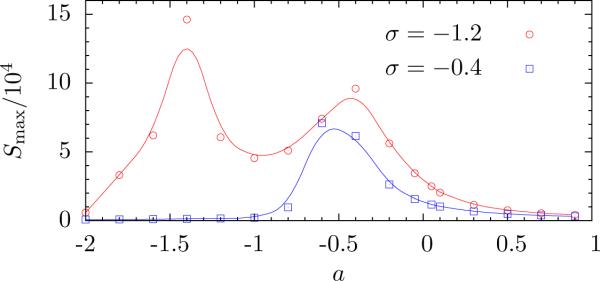
The maximum of the structure factor, Smax, as a function of a. For σ = −0.4, only one peak is observed, corresponding to the transition from the microemulsion fluid to the coexisting phase. For σ = −1.2, there are two transitions, one from the microemulsion to the modulated phase, and one from there to coexisting phases. Symbols are simulation results, and solid lines are spline interpolations of the data.
Note that in a first order transition, increasing fluctuations are generally a signature of the spinodal line; the line where the metastable state loses its stability. However, close to the tricritical point the spinodal line is close the the transition line. Far from the tricritical point one can compare the mean energy of the two stable states, where the point of equal energy denotes the first order transition.
Fig. 4 shows Smax for two cases with σ < 0. The first case, where σ is close to zero, shows only one peak in Smax. The second case of σ < < 0, shows two peaks as expected from the mean field approximation. Calculating kmax, we find that the former corresponds to a transition from the microemulsion phase to two-phase coexistence. This transition does not exist in the mean field approximation. It suggests that systems which show phase separation can support the formation of a microemulsion.
P (ϕ) and confirm that the transition is from a microemulsion phase directly to two-phase coexistence if σ is negative but not too, small, while for σ ≲ −1 there are two transitions: one from a microemulsion to a modulated phase, and one from there to two-phase coexistence.
To find the first order transition far from the tricritical point, we calculate the mean energy, 〈Etot〉, as a function of a, starting from two different stable states of the system. Plotting the two curves 〈Etot〉 vs. a, the point of intersection indicates the triple line. Close to the tricritical point, the slope of the two curves are very similar, and the intersection point is difficult to determine. Hence, we use the peak of the structure factor to identify the transition, as described above.
Figure 5 shows a time frame from the simulation near the critical line. In the first case, the system temperature a is raised and the system stays in a uniform state, while in the second the temperature is reduced and the system remains in a modulated phase. This shows, as expected, that near the first order transition the final state depends on the way the system was prepared. We show S(k), , and the the distribution P(ϕ) for each phase.
Figure 5.

Hysteresis is a signature of a first order transition. Both top and bottom panels correspond to a = −1.5 and σ = −1.2, but were prepared by changing the effective temperature from below (top panel) and from above (bottom panel). Each panel shows a snapshot of a typical configuration, the structure factor S(k) and the magnitude of the average Fourier mode (each in arbitrary units), and the distribution P(ϕ).
To summarize this section, we find that our simple model can explain different structures observed on membranes: the transition of a uniform phase to two coexisting phases, and the formation of modulated phases like stripes and hexagonal phase. Including the effects of fluctuations, we find that the critical temperature is reduced, and that there is a direct transition from a microemulsion fluid to two-phase coexistence. Lastly, we show that as a modulated phase melts to a uniform phase, this phase is a microemulsion with a characteristic length scale that resembles that of the modulated phase.
4. Application: Hybrid models
At length scales much larger than its thickness, a biological membrane behaves like a two-dimensional fluid sheet, and its properties are dominated by two material constants: surface tension and bending rigidity. By treating the membrane as a two-dimensional surface embedded in three-dimensional space, one can derive computationally efficient models of membrane shape dynamics, which we will interface with a general model of membrane-associated proteins.
4.1. General Elastic Model
The standard model for understanding the shape and fluctuations of a biological membrane was developed by Canham and Helfrich [10, 11, 38, 39]. It asserts that the energy of membrane conformation can be written as
| (39) |
where σ and κ are the surface tension and bending rigidity, respectively, R1 and R2 are the principal radii of curvature, C0 is the spontaneous curvature, kg is the saddle-splay modulus, and the integral is taken over the membrane surface.
According to the Gauss-Bonnet theorem, the Gaussian curvature term in (39) is a topological invariant. Because the membrane topology cannot change within our model, this term merely adds a constant to the total energy and can therefore be discarded. For simplicity we will focus on membranes without spontaneous curvature, C0 = 0, such as a homogeneous symmetric bilayer.
We limit ourselves to membrane conformations that are deviations from a completely flat membrane without overhangs. In this case, the shape of the membrane can be parametrized by a single height function h(r), where r = (x, y). This is known as the Monge gauge representation. If the deviations from the reference shape are small, then we can expand the energy (39) to quadratic order in h and its derivatives, and finally obtain
| (40) |
This expression is a special case of the general energy functional (1), where ϕ(r) has been replaced with h(r). Following the procedure outlined in Section 2.3, we express the energy in terms of the Fourier components of the membrane height field:
| (41) |
This transformation implies the use of periodic boundary conditions. The equation of motion for the Fourier coefficients is the Langevin equation
| (42) |
| (43) |
In these expressions is the Fourier transform of the Oseen tensor, which accounts for the viscosity of the surroundings. It plays the role of a generalized mobility in the Langevin equation that captures hydrodynamic effects. For a membrane surrounded by a solvent of viscosity η it takes the form: [16, 39]
| (44) |
The last term in (43) is a Gaussian stochastic noise term that satisfies the fluctuation-dissipation theorem (20):
| (45) |
| (46) |
The dynamical scheme encoded in these equations is known as Fourier Space Brownian Dynamics [16, 39–41]. In the present form it simulates the dynamics of a free membrane embedded in implicit solvent. After integrating (43), information about the thermal fluctuations of the membrane is obtained. From the equipartition theorem, the average fluctuations of the membrane height are given by
| (47) |
Obtaining this fluctuation spectrum is an important test for the correctness and convergence of a computer simulation of the dynamics of a free membrane.
4.2. Hybrid Membrane–Particle model
While the structure and dynamics of a free membrane is well understood within the Canham-Helfrich framework, there has been recent interest in coupling this model with a particle description of other cellular components, such as membrane proteins. Trying to combine a continuum representation with a discrete representation poses severe challenges both in the mathematical formulation and in the computational implementation of such models.
We are guided in the development of our model by the interaction between the plasma membrane and the actin cytoskeleton. The presence of actin filaments locally quenches membrane fluctuations, mainly due to steric interactions. For simplicity we will neglect all chemical detail of the filaments, and only maintain the position at which the membrane height is pinned to a specific value by the protein. This system is illustrated in Fig. 6.
Figure 6.
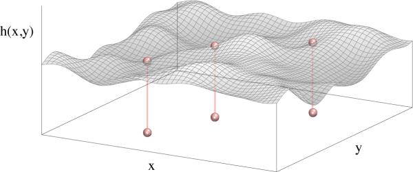
Schematic of a membrane configuration in the Monge gauge. The membrane shape is parametrized by the function h(x, y). Proteins diffusing in the (x,y) plane impose local harmonic constraints on the membrane height.
In our model, the energy of the system can be decomposed into a contribution from the free membrane, membrane-protein interactions, and protein-protein interactions:
| (48) |
The first term is the energy of the free membrane, (41). The second term represents the coupling of the membrane with the proteins, which we write as
| (49) |
Here, the two-dimensional vector ri is the location at which protein i limits the membrane height to small fluctuations around the fixed length l. The parameter ε describes the strength of the constraint imposed by the protein.
The equation of motion for the membrane height is derived using the Langevin formalism described in Section 2.3. In the presence of membrane-protein coupling, equation (15) becomes
| (50) |
For the protein-protein interaction we assume a pairwise additive potential that depends only on the separation between two proteins,
| (51) |
where V(r) is the pair potential. We choose a generic and purely repulsive potential that has the functional form of the Weeks-Chandler-Andersen (WCA) potential [42],
| (52) |
The parameters εpp and σpp set the energy and length scale for the protein-protein interaction, respectively.
We still need to specify the dynamics for the filaments. We assume that they undergo Brownian motion in the (x, y) plane, governed by the Langevin equation
| (53) |
Here ∇iEtotal is the gradient of the energy with respect to the position of particle i and γp is the mobility coefficient. The latter is related to the bare diffusion constant through D0 = kBTγp. Evaluating the gradient yields
| (54) |
We note that the gradient of the height field is given by
| (55) |
The final term in (53) is a stochastic force acting on protein i. Its statistics are governed by the fluctuation-dissipation theorem
| (56) |
where α and β denote the Cartesian components of the vector ζi.
Numerically integrating equations (50) and (54) in time allows us to simulate the time evolution of both membrane geometry and protein positions. For this we need to choose a time step, Δt, that is small enough to resolve all pertinent dynamic processes [17]. There are multiple bounds to the time-step that must be considered. The first depends on the relaxation time (21) of the fastest membrane mode in the system, which requires that
| (57) |
where kmax is the largest wavevector in the system. To avoid proteins moving over distances comparable to their diameter in a single timestep, we also require . Similarly, the distance travelled in a single timestep should be small compared to the shortest wavelength of the membrane Fourier modes, .
At this point we emphasize similarities and differences with existing hybrid models. The effect of locally suppressing membrane height fluctuations at static pinning sites has been studied in Ref. [16] to investigate the role of the spectrin network on the membrane of red blood cells. The diffusion of single inclusions within the membrane has been investigated in Refs. [19–21]. In these studies, the protein is coupled to the membrane curvature, rather than the membrane height. The effect of multiple proteins that locally pin the membrane height to fixed values has been studied in a lattice model [43, 44]. In our model, we focus on the effect of the membrane on the structure of proteins diffusing in the (x, y) plane.
Our approach also differs in details of the numerical implementation. Most authors use the DFT to convert the membrane Fourier modes to real space. This results in a sampling of the height field h(r) on a regular grid. If the proteins diffuse in the continuum, one must interpolate those sampling points, which can result in artifacts that must be corrected [21, 22]. Since the number of proteins is relatively small, we instead use equations (13) and (55) directly to compute the membrane height and its derivative at the positions of the proteins.
To quantify the effect of the membrane-induced interaction among the proteins, we calculate the radial distribution function
| (58) |
which is a measure of correlations among proteins.
This function is shown in Figure 7 for a membrane with N = 100 proteins. If the bending rigidity is infinite, then the membrane is completely flat, and the proteins behave like a two-dimensional WCA fluid. Lowering κ, and thereby increasing membrane fluctuations, leads to a broad peak at a distance r ≳ σpp. This illustrates the attractive nature of membrane-induced attractions that originate from suppressing membrane fluctuations.
Figure 7.

Protein pair correlation function for density, and varying values of κ/kBT. The surface tension σ was set to zero, and strength of the membrane-protein interaction ε = 100kBT. Lowering the bending rigidity leads to an accumulation of proteins.
5. Discussion and Outlook
The present work illustrates how modeling of either the composition or the shape as a continuum field can shed light on the complicated behavior of biological membranes at large length scales. A natural question to ask is whether additional phenomena set in when one follows the coupled dynamics of both fields explicitly. Experiments suggest that there are indeed situations where these distinct physical quantities are tightly coupled, see for example Refs. [45–48]. While both fields were considered in Section 3.1, integrating over the shape fluctuations implies that these geometric degrees of freedom are constantly in equilibrium, which might not always be the case in an experimental systems. Using the methods outlined in Section 2, it is straightforward to study the coupled dynamics of both fields [49, 50].
The plasma membrane is asymmetric, i.e., the chemical compositions of the inner and the outer leaflet differ significantly. Therefore, the leaflets can have different tendencies to phase separate or to exhibit other forms of spatial organization. This is also true for the coupling of each leaflet's composition to the shape of the membrane. These effects can be captured in models with not one, but two composition fields (one for each leaflet). Coupling of these fields gives rise to complex phenomena that are currently being explored [51, 52].
To study the effect of membrane-mediated interactions between proteins, we have presented a hybrid model that couples a continuum description of the membrane with a particle representation of the proteins. We have assumed a form of the protein-membrane interaction that describes a harmonic constraint on the membrane height above a reference plane, as is appropriate for proteins that suppress height fluctuations. Other proteins, such as sca olding proteins [13], can couple to other geometric quantities of the membrane, for example its curvature. Hybrid models that take such coupling into account have been developed in Refs. [19, 21, 22]. While we have focused on proteins whose interaction can be described by a generic isotropic pair potential, it is desirable to incorporate into the model more complicated protein–protein interactions. The first step in this direction would be to endow proteins with rotational, in addition to translational, degrees of freedom, for example in a rigid body framework of protein motion.
While continuum models of the membrane are the central topic of this report, we would like to end with a brief discussion of particle models of biological membranes. The recent development of coarse-grained force fields has significantly increased the length scale accessible to molecular modeling techniques. Membranes consisting of thousands of lipid molecules can be simulated over microsecond timescales with models that maintain a significant degree of chemical fidelity, such as the Martini force field [53, 54]. This allows the simulation of phase separation processes over tens of nanometers. Even bigger system sizes can be used with more aggressively coarse-grained and solvent-free models [55–57]. For example, a microsecond simulation of a 120 nm diameter vesicle has recently been reported [56]. While each lipid molecule is represented in these models by so few degrees of freedom that further coarse-graining at the molecular level seems unlikely, it is possible to design particle models in which each fundamental unit represents multiple lipid molecules or small patches of membrane [58–62]. These models accurately reproduce the mesoscopic elastic properties of membranes, and can therefore complement continuum models to study the coupling of membrane shape and protein organization.
Figure 3.
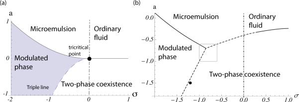
Phase diagram of the model calculated within the mean-field approximation (a), and using our numerical methods (b), in terms of the two parameters a and σ. Dashed lines denote first-order transitions, solid lines continuous ones. The region of macroscopic phase separation is denoted “two-phase coexistence.” The dash-dot line is the Lifshitz line. To the right of it the fluid is an ordinary one, while to the left of it the fluid is a microemulsion. The solid circle in panel (a) shows the tricritical point, and that in (b) shows the parameters used in Fig. 5.
Acknowledgments
We thank Michael Schick and Sarah Keller for many insightful discussions. Research reported in this publication was supported by the National Institute of General Medical Sciences of the National Institutes of Health under award number T32GM008268 (K. S.) and by a fellowship from the Raymond and Beverly Sackler Foundation (R. S.).
References
- 1.Singer SJ, Nicolson GL. The fluid mosaic model of the structure of cell membranes. Science. 1972;175(4023):720–731. doi: 10.1126/science.175.4023.720. [DOI] [PubMed] [Google Scholar]
- 2.Pike LJ. Rafts defined: a report on the keystone symposium on lipid rafts and cell function. J. Lip. Res. 2006;47:1597–1598. doi: 10.1194/jlr.E600002-JLR200. [DOI] [PubMed] [Google Scholar]
- 3.Lingwood D, Simons K. Lipid rafts as a membrane-organizing principle. Science. 2010;327(5961):46–50. doi: 10.1126/science.1174621. [DOI] [PubMed] [Google Scholar]
- 4.Veatch SL, Keller SL. Organization in lipid membranes containing cholesterol. Phys. Rev. Lett. 2002;89:268101. doi: 10.1103/PhysRevLett.89.268101. [DOI] [PubMed] [Google Scholar]
- 5.Veatch SL, Keller SL. Separation of liquid phases in giant vesicles of ternary mixtures of phospholipids and cholesterol. Biophys. J. 2003;85:3074. doi: 10.1016/S0006-3495(03)74726-2. [DOI] [PMC free article] [PubMed] [Google Scholar]
- 6.McConnell HM, Vrljic M. Liquid–liquid immiscibility in membranes. Ann. Rev. Biophys. Biochem. 2003;32:469–492. doi: 10.1146/annurev.biophys.32.110601.141704. [DOI] [PubMed] [Google Scholar]
- 7.Simons K, Vaz WLC. Model systems, lipid rafts, and cell membranes. Ann. Rev. Biophys. Biomol. Struct. 2004;33:269–295. doi: 10.1146/annurev.biophys.32.110601.141803. [DOI] [PubMed] [Google Scholar]
- 8.Veatch SL, Keller SL. Seeing spots: Complex phase behavior in simple membranes. Biochim. Biophys. Acta – Molecular Cell Research. 2005;1746(3):172–185. doi: 10.1016/j.bbamcr.2005.06.010. [DOI] [PubMed] [Google Scholar]
- 9.Goldenfeld N. Lectures on Phase Transitions and the Renormalization Group. Perseus Books Publishing; 1992. [Google Scholar]
- 10.Canham PB. The minimum energy of bending as a possible explanation of the biconcave shape of the red blood cell. J. Theor. Biol. 1970;26:61–81. doi: 10.1016/s0022-5193(70)80032-7. [DOI] [PubMed] [Google Scholar]
- 11.Helfrich W. Elastic properties of lipid bilayers - theory and possible experiments. Z. Naturforsch. C. 1973;28:693–703. doi: 10.1515/znc-1973-11-1209. [DOI] [PubMed] [Google Scholar]
- 12.Seifert U. Configurations of fluid membranes and vesicles. Adv. Phys. 1997;46(1):13–137. [Google Scholar]
- 13.Frost A, Unger VM, de Camilli P. Aspenström P, editor. Boomerangs, bananas and blimps: Structure and function of FBAR domains in the context of the BAR domain superfamily. The Pombe Cdc15 Homology Proteins, Landes Bioscience. 2009 [Google Scholar]
- 14.Liu AP, Richmond DL, Maibaum L, Pronk S, Geissler PL, Fletcher DA. Membrane-induced bundling of actin filaments. Nature Physics. 2008;4:789–793. doi: 10.1038/nphys1071. [DOI] [PMC free article] [PubMed] [Google Scholar]
- 15.Kloeden PE, Platen E. Numerical Solutions of Stochastic Differential Equations. Springer; 1992. [Google Scholar]
- 16.Lin LC-L, Brown FLH. Dynamic simulations of membranes with cytoskeletal interactions. Phys. Rev. E. 2005;72:011910. doi: 10.1103/PhysRevE.72.011910. [DOI] [PubMed] [Google Scholar]
- 17.Reister-Gottfried E, Leitenberger SM, Seifert U. Hybrid simulations of lateral diffusion in fluctuating membranes. Phys. Rev. E. 2007;75(1):011908. doi: 10.1103/PhysRevE.75.011908. [DOI] [PubMed] [Google Scholar]
- 18.Camley BA, Brown FLH. Dynamic simulations of multicomponent lipid membranes over long length and time scales. Phys. Rev. Lett. 2010;105:148102. doi: 10.1103/PhysRevLett.105.148102. [DOI] [PubMed] [Google Scholar]
- 19.Leitenberger SM, Reister-Gottfried E, Seifert U. Curvature coupling dependence of membrane protein diffusion coe cients. Langmuir. 2008;24(4):1254–1261. doi: 10.1021/la702319q. [DOI] [PubMed] [Google Scholar]
- 20.Reister-Gottfried E, Leitenberger SM, Seifert U. Diffusing proteins on a fluctuating membrane: Analytical theory and simulations. Phys. Rev. E. 2010;81(3):031903. doi: 10.1103/PhysRevE.81.031903. [DOI] [PubMed] [Google Scholar]
- 21.Naji A, Atzberger PJ, Brown FLH. Hybrid elastic and discrete-particle approach to biomembrane dynamics with application to the mobility of curved integral membrane proteins. Phys. Rev. Lett. 2009;102:138102. doi: 10.1103/PhysRevLett.102.138102. [DOI] [PubMed] [Google Scholar]
- 22.Sigurdsson JK, Brown FLH, Atzberger PJ. Hybrid continuum-particle method for fluctuating lipid bilayer membranes with diffusing protein inclusions. J. Comp. Phys. 2013;252:65–85. [Google Scholar]
- 23.Boyd JP. Chebyshev and Fourier Spectral Methods. Dover; 2001. [Google Scholar]
- 24.If the nonlinearity was quadratic rather than cubic, the padding would instead have to satisfy the inequality P + p > (3/2)P, which is known as Orszag's “Three-Halves Rule”[23, 63].
- 25.Simons K, Van Meer G. Lipid sorting in epithelial cells. Biochem. 1988;27(17):6197–6202. doi: 10.1021/bi00417a001. [DOI] [PubMed] [Google Scholar]
- 26.Schick M. Membrane heterogeneity: Manifestation of a curvature-induced microemulsion. Phys. Rev. E. 2012;85:031902. doi: 10.1103/PhysRevE.85.031902. [DOI] [PubMed] [Google Scholar]
- 27.Komura S, Andelman D. Physical aspects of heterogeneities in multi-component lipid membranes. Adv. Colloid Interface Sci. 2014 doi: 10.1016/j.cis.2013.12.003. in press. [DOI] [PubMed] [Google Scholar]
- 28.Brewster R, Pincus PA, Safran SA. Hybrid lipids as a biological surface-active component. Biophys. J. 2009;97(4):1087–1094. doi: 10.1016/j.bpj.2009.05.051. [DOI] [PMC free article] [PubMed] [Google Scholar]
- 29.Yamamoto T, Brewster R, Safran SA. Chain ordering of hybrid lipids can stabilize domains in saturated/hybrid/cholesterol lipid membranes. Europhys. Lett. 2010;91(2):28002. [Google Scholar]
- 30.Palmieri B, Safran SA. Hybrid lipids increase the probability of fluctuating nanodomains in mixed membranes. Langmuir. 2013;29(17):5246–5261. doi: 10.1021/la4006168. [DOI] [PubMed] [Google Scholar]
- 31.Toulmay A, Prinz WA. Direct imaging reveals stable, micrometer-scale lipid domains that segregate proteins in live cells. J. Cell. Biol. 2013;202(1):35. doi: 10.1083/jcb.201301039. [DOI] [PMC free article] [PubMed] [Google Scholar]
- 32.Spira F, Mueller NS, Beck G, von Olshausen P, Beig J, Wedlich-Söldner R. Patchwork organization of the yeast plasma membrane into numerous coexisting domains. Nature Cell Bio. 2012;14:640–648. doi: 10.1038/ncb2487. [DOI] [PubMed] [Google Scholar]
- 33.Hornreich RM, Luban M, Shtrikman S. Critical behavior at the onset of k-space instability on the lambda line. Phys. Rev. Lett. 1975;35:1678. [Google Scholar]
- 34.Swift J, Hohenberg PC. Hydrodynamic fluctuations at the convective instability. Phys. Rev. A. 1977;15:319. [Google Scholar]
- 35.Kumar PBS, Gompper G, Lipowsky R. Modulated phases in multicomponent fluid membranes. Phys. Rev. E. 1999;60:4610–4618. doi: 10.1103/physreve.60.4610. [DOI] [PubMed] [Google Scholar]
- 36.Hirose H, Takeuchi T, Osakada H, Pujals S, Katayama S, Nakase I, Kobayashi S, Haraguchi T, Futaki S. Transient focal membrane deformation induced by arginine-rich peptides leads to their direct penetration into cells. Molecular Therapy. 2012;20(5):984–993. doi: 10.1038/mt.2011.313. [DOI] [PMC free article] [PubMed] [Google Scholar]
- 37.Shlomovitz R, Maibaum L, Schick M. Macroscopic phase separation, modulated phases, and microemulsions: A unified picture of rafts. Biophys. J. 2014 doi: 10.1016/j.bpj.2014.03.017. in press. [DOI] [PMC free article] [PubMed] [Google Scholar]
- 38.Safran SA. Statistical Thermodynamics of Surfaces, Interfaces and Membranes. Addison–Wesley Publishing; 1994. [Google Scholar]
- 39.Brown FLH. Elastic modeling of biomembranes and lipid bilayers. Ann. Rev. Phys. Chem. 2008;59:685–712. doi: 10.1146/annurev.physchem.59.032607.093550. [DOI] [PubMed] [Google Scholar]
- 40.Lin LC-L, Brown FLH. Brownian dynamics in fourier space: Membrane simulations over long length and time scales. Phys. Rev. Lett. 2004;93:256001. doi: 10.1103/PhysRevLett.93.256001. [DOI] [PubMed] [Google Scholar]
- 41.Brown FLH. Continuum simulations of biomembrane dynamics and the importance of hydrodynamic effects. Quarterly Reviews of Biophysics. 2011;44(4):391–432. doi: 10.1017/S0033583511000047. [DOI] [PubMed] [Google Scholar]
- 42.Weeks JD, Chandler D, Andersen HC. Role of repulsive forces in determining the equilibrium structure of simple liquids. J. Chem. Phys. 1971;54:5237. [Google Scholar]
- 43.Speck T, Reister E, Seifert U. Specific adhesion of membranes: Mapping to an effective bond lattice gas. Phys. Rev. E. 2010;82:021923. doi: 10.1103/PhysRevE.82.021923. [DOI] [PubMed] [Google Scholar]
- 44.Speck T. Effective free energy for pinned membranes. Phys. Rev. E. 2011;83:050901(R). doi: 10.1103/PhysRevE.83.050901. [DOI] [PubMed] [Google Scholar]
- 45.Baumgart T, Hess ST, Webb WW. Imaging coexisting fluid domains in biomembrane models coupling curvature and line tension. Nature. 2003;425:821. doi: 10.1038/nature02013. [DOI] [PubMed] [Google Scholar]
- 46.Parthasarathy R, Yu C-H, Groves JT. Curvature–modulated phase separation in lipid bilayer membranes. Langmuir. 2006;22(11):5095–5099. doi: 10.1021/la060390o. [DOI] [PubMed] [Google Scholar]
- 47.Yanagisawa M, Imai M, Masui T, Komura S, Ohta T. Growth dynamics of domains in ternary fluid vesicles. Biophys. J. 2007;92:115–125. doi: 10.1529/biophysj.106.087494. [DOI] [PMC free article] [PubMed] [Google Scholar]
- 48.Groves JT. Bending mechanics and molecular organization in biological membranes. Ann. Rev. Phys. Chem. 2007;58:697–717. doi: 10.1146/annurev.physchem.56.092503.141216. [DOI] [PubMed] [Google Scholar]
- 49.Taniguchi T. Shape deformation and phase separation dynamics of two-component vesicles. Phys. Rev. Lett. 1996;76:4444–4447. doi: 10.1103/PhysRevLett.76.4444. [DOI] [PubMed] [Google Scholar]
- 50.Wada H. Dynamics of phase separation in confined two-component fluid membranes. J. Phys. Soc. Jap. 2003;72(12):3142–3150. [Google Scholar]
- 51.Shlomovitz R, Schick M. Model of a raft in both leaves of an asymmetric lipid bilayer. Biophys. J. 2013;105:1406–1413. doi: 10.1016/j.bpj.2013.06.053. [DOI] [PMC free article] [PubMed] [Google Scholar]
- 52.Funkhouser CM, Mayer M, Solis FJ, Thornton K. Effects of interleaflet coupling on the morphologies of multicomponent lipid bilayer membranes. J. Chem. Phys. 2013;138:024909. doi: 10.1063/1.4773856. [DOI] [PubMed] [Google Scholar]
- 53.Marrink SJ, Risselada HJ, Yefimov S, Tieleman DP, de Vries AH. The MARTINI force field: Coarse grained model for biomolecular simulations. J. Phys. Chem. B. 2007;111(27):7812–7824. doi: 10.1021/jp071097f. [DOI] [PubMed] [Google Scholar]
- 54.Marrink SJ, Tieleman DP. Perspective on the martini model. Chem. Soc. Rev. 2013;42:6801–6822. doi: 10.1039/c3cs60093a. [DOI] [PubMed] [Google Scholar]
- 55.Wang Z-J, Deserno M. A systematically coarse-grained solvent-free model for quantitative phospholipid bilayer simulations. J. Phys. Chem. B. 2010;114(34):11207–11220. doi: 10.1021/jp102543j. [DOI] [PMC free article] [PubMed] [Google Scholar]
- 56.Srivastava A, Voth GA. Hybrid approach for highly coarse-grained lipid bilayer models. J. Chem. Theo. Comp. 2013;9(1):750–765. doi: 10.1021/ct300751h. [DOI] [PMC free article] [PubMed] [Google Scholar]
- 57.Simunovic M, Srivastava A, Voth GA. Linear aggregation of proteins on the membrane as a prelude to membrane remodeling. Proc. Natl. Acad. Sci. USA. 2013;110(51):20396–20401. doi: 10.1073/pnas.1309819110. [DOI] [PMC free article] [PubMed] [Google Scholar]
- 58.Drouffe J-M, Maggs AC, Leibler S. Computer simulations of self-assembled membranes. Science. 1991;254(5036):1353–1356. doi: 10.1126/science.1962193. [DOI] [PubMed] [Google Scholar]
- 59.Chang R, Ayton GS, Voth GA. Multiscale coupling of mesoscopic- and atomistic-level lipid bilayer simulations. J. Chem. Phys. 2005;122:244716. doi: 10.1063/1.1931651. [DOI] [PubMed] [Google Scholar]
- 60.Ayton GS, McWhirter JL, Voth GA. A second generation mesoscopic lipid bilayer model: Connections to field-theory descriptions of membranes and nonlocal hydrodynamics. J. Chem. Phys. 2006;124:064906. doi: 10.1063/1.2165194. [DOI] [PubMed] [Google Scholar]
- 61.Noguchi H, Gompper G. Dynamics of vesicle self-assembly and dissolution. J. Chem. Phys. 2006;125:164908. doi: 10.1063/1.2358983. [DOI] [PubMed] [Google Scholar]
- 62.Pasqua A, Maibaum L, Oster G, Fletcher DA, Geissler PL. Large-scale simulations of fluctuating biological membranes. J. Chem. Phys. 2010;132:154107. doi: 10.1063/1.3382349. [DOI] [PMC free article] [PubMed] [Google Scholar]
- 63.Orszag SA. On the elimination of aliasing in finite-difference schemes by filtering high-wavenumber. J. Atmos. Sci. 1971;28:1074. [Google Scholar]