

Abstract
Purpose
To remove nuisance signals (e.g., water and lipid signals) for 1H MRSI data collected from the brain with limited and/or sparse (k, t)-space coverage.
Methods
A union-of-subspace model is proposed for removing nuisance signals. The model exploits the partial separability of both the nuisance signals and the metabolite signal, and decomposes an MRSI dataset into several sets of generalized voxels that share the same spectral distributions. This model enables the estimation of the nuisance signals from an MRSI dataset that has limited and/or sparse (k, t)-space coverage.
Results
The proposed method has been evaluated using in vivo MRSI data. For conventional CSI data with limited k-space coverage, the proposed method produced “lipid-free” spectra without lipid suppression during data acquisition at 130 ms echo time. For sparse (k, t)-space data acquired with conventional pulses for water and lipid suppression, the proposed method was also able to remove the remaining water and lipid signals with negligible residuals.
Conclusions
Nuisance signals in 1H MRSI data reside in low-dimensional subspaces. This property can be utilized for estimation and removal of nuisance signals from 1H MRSI data even when they have limited and/or sparse coverage of (k, t)-space. The proposed method should prove useful especially for accelerated high-resolution 1H MRSI of the brain.
Keywords: 1H spectroscopic imaging, chemical shift imaging, sparse sampling, lipid removal, water removal, partial separability, union of subspaces
Introduction
In 1H MRSI experiments, especially of the brain, it is necessary to remove the nuisance signals (e.g., the water and lipid signals) because they are often orders of magnitude stronger than the desired metabolite signal. Many methods have been proposed for suppression of the nuisance signals during data acquisition by exploiting the differences between the nuisance and metabolite signals in resonance frequency, spatial support, and relaxation parameters. For example, water suppression can be achieved using chemical shift-selective saturation (CHESS) pulses (1–5), and lipid signals can be suppressed using long echo-time (TE) acquisition, outer-volume-suppression (OVS) (6, 7), inversion recovery (8, 9), and selective excitation of the brain region (10, 11). However, the usefulness of these methods is often limited by practical conditions (e.g., B0 and B1 inhomogeneities).
Alternatively, post-processing methods can be used for removing nuisance signals. In conventional, fully-sampled chemical shift imaging (CSI, (12)) acquisitions, linear predictive methods (e.g., HSVD (13)) are effective for removing the water signal. However, removing the lipid signal (e.g., from the subcutaneous layer of the brain) is more difficult if the MRSI data cover only limited k-space, as is often the case in CSI acquisitions, where resolution is typically sacrificed in order to maintain a short scan time. One approach is to use prior knowledge of the lipid and metabolite signals, such as the spatial support of the lipid signal (14–17), the spectral support of the metabolite signal (18, 19), and sparsity (20). Another approach is to merge low-resolution MRSI data with a high-resolution lipid estimate (obtained in a short auxiliary scan) (20–24). While a complete removal of the lipid signal is difficult for limited k-space data, the problem becomes more challenging when (k, t)-space is sparsely sampled as is the case with recent accelerated MRSI techniques (25–27).
In this work, we address the nuisance signal removal problem using a union-of-subspaces model. The proposed model exploits the partial separability (PS) properties of both the nuisance signals and the metabolite signal (28–30) and decomposes an MRSI dataset into several sets of generalized voxels that share the same spectral distributions. This model enables the estimation and removal of the nuisance signals from MRSI data that have limited and/or sparse (k, t)-space coverage. We demonstrate the effectiveness of the proposed method using in vivo MRSI data collected from healthy volunteers on a 3.0 T MRI scanner. We show that the proposed method produced “lipid-free” spectra for a CSI dataset acquired at 130 ms TE with 16 × 16 spatial encodings and no extra lipid suppression. We also show that the proposed method removed the remaining water and lipid signals (after nominal water and lipid suppression) with negligible residuals from a sparse (k, t)-space dataset that was acquired using an echo-planar spectroscopic imaging (EPSI (31)) sequence. A preliminary account of this work was presented in (32).The MATLAB codes and data for generating the results in the paper are made available online at http://mri.beckman.uiuc.edu/software.html.
Theory
In this section, we first introduce the proposed union-of-subspaces model and then describe a general framework to estimate nuisance signals from measured data using the proposed model, followed by procedures for removing nuisance signals from 1) limited k-space data, 2) sparse (k, t)-space data, and 3) hybrid data comprising of two datasets that have limited and sparse (k, t)-space coverage, respectively.
Union-of-subspaces modeling
We decompose the desired spatial-temporal signal ρ(x, t) of an MRSI experiment as
| [1] |
where ρM(x, t) represents the desired metabolite signal, ρL(x, t) the lipid signal, and ρW(x, t) the water signal. The model in Eq. [1] indicates that ρM(x, t) resides in a subspace (denoted as
 M) spanned by a set of temporal basis
with spatial coefficients
, ρL(x, t) in a subspace (denoted as
L) spanned by a set of temporal basis
with spatial coefficients
, and ρW(x, t) in a subspace (denoted as
W) spanned by a set of temporal basis
with spatial coefficients
. Therefore, ρM(x, t), ρL(x, t) and ρW(x, t) reside in the union of
M,
L and
W, and Eq. [1] is called a union-of-subspaces model. Note that ρ(x, t) resides in the sum of
M,
L and
W, and is not a union-of-subspaces signal in the strict sense of (33).
M) spanned by a set of temporal basis
with spatial coefficients
, ρL(x, t) in a subspace (denoted as
L) spanned by a set of temporal basis
with spatial coefficients
, and ρW(x, t) in a subspace (denoted as
W) spanned by a set of temporal basis
with spatial coefficients
. Therefore, ρM(x, t), ρL(x, t) and ρW(x, t) reside in the union of
M,
L and
W, and Eq. [1] is called a union-of-subspaces model. Note that ρ(x, t) resides in the sum of
M,
L and
W, and is not a union-of-subspaces signal in the strict sense of (33).
Without assuming any prior structure of the subspaces, it very challenging to recover each signal component from a given dataset that has limited and/or sparse (k, t)-space coverage. The proposed model provides necessary means to incorporate prior knowledge of the water, lipid and metabolite signals and thus enables the estimation of the nuisance and metabolite signals from such data. For the metabolite signal, the resonance frequencies of most detectable metabolites of the human brain are between 0.5 ∼ 4.2 ppm (34), and the spatial support is the brain region. The lipid signal originates from multiple regions surrounding the brain, especially the subcutaneous layer of the head; and its spectrum consists of multiple peaks between 0.9 ∼ 5.7 ppm with a main peak at 1.3 ppm (35). These peaks are broad due to short T2 and large magnetic field inhomogeneities near the air/tissue boundary.
The key issue of using the proposed model for removing nuisance signals is to determine the temporal basis of each subspace and the corresponding spatial coefficients. In the following, we first describe a general approach to determining the temporal bases and the spatial coefficients and then discuss specific procedures to remove nuisance signals in conventional and accelerated MRSI.
Determination of the temporal bases
The use of the union-of-subspaces model in the proposed method first depends on determining the temporal basis for each subspace in Eq. [1]. Without any additional prior knowledge, determination of the temporal bases requires (k, t)-space data satisfying both the temporal and spatial Nyquist criteria. If each signal component can be separated from such (k, t)-space data, determining the temporal basis for each subspace is straightforward and has been described in previous works (28). However, there are two practical issues faced by our proposed method: a) the presence of magnetic field inhomogeneities, and b) estimation from data with limited k-space coverage.
In the presence of magnetic field inhomogeneities, the measured (k, t)-space data can be expressed as
| [2] |
where Δf(x) is the frequency shift due to magnetic field inhomogeneity, and ε(k, t) is the measurement noise (often assumed to be white Gaussian). The field inhomogeneity results in spectral shift and lineshape distortion in the Fourier transform reconstructed MRSI data, and the union-of-subspaces model in Eq. [1] is a poor approximation of such a reconstruction. The proposed method uses a separately acquired magnetic field map to correct for field inhomogeneity using the conjugate phase method (36, 37) prior to estimating the temporal bases.
Another practical issue is limited k-space coverage. Ideally, the lipid and metabolite signal can be separated from each other based on their distinct spatial supports; however, the leakage of the lipid signal due to limited k-space coverage can be significant. To address this issue, we exploit the prior knowledge of the spectra of the lipid and metabolite signals. More specifically, to separate the lipid signal, the water signal is first separated from the lipid and metabolite signals based on its distinct spectral support using the HSVD method. The spatial mask of the lipid signal (e.g., comprising the subcutaneous fat layer) is then applied, and the HSVD method is used to extract the lipid signal at each voxel of the masked data based on its known resonance frequencies and short value. The metabolite signal can be extracted similarly.
After each signal component is separated, the temporal bases are determined by constructing the corresponding Casorati matrices followed by singular value decomposition (SVD). For example, suppose the extracted lipid signal ρ̃L(x, t) is defined over a grid , its Casorati matrix is given by
| [3] |
The temporal basis of the lipid signal is chosen to be the PL most significant right-singular vectors of C(ρ̃L).
We determine the model order PL by examining the singular values of C(ρ̃L) (denoted as σL,p, p = 1, 2, …). Assuming the measurement noise is i.i.d Gaussian noise and its standard deviation is known, the Marchenko-Pastur distribution can be used to estimate the singular values of the Casorati matrix formed by the measurement noise (30, 38). Suppose the largest singular value of the Casorati matrix of the noise is σ0, we choose PL so that
| [4] |
Determination of the spatial coefficients
After the temporal bases are determined, the remaining problem is to determine the spatial coefficients ( in Eq. [1]) from the given (k, t)-space data, which can have limited or sparse (k, t)-space coverage. The spatial coefficients can be estimated by fitting the given data using the proposed model in Eq. [1], while incorporating the prior knowledge of the spatial supports of different signals for better estimation.
More specifically, suppose the estimated temporal bases are , the desired signal can be written as
| [5] |
where WM(x), WL(x), and WW(x) represent the spatial supports of the metabolite, lipid and water signals, respectively.
Discretizing Eq. [5] and substituting to the signal equation Eq. [2], yields the following optimization problem to determine the spatial coefficients (25, 32):
| [6] |
where the first term describes data consistency, the second term is a regularization penalty with parameter λ, s is a vector containing the (k, t)-space data, Ω is the corresponding sampling operator, FB is a discrete Fourier transform operator including the field inhomogeneity induced phase term as in Eq. [2], W = diag{WW, WL, WM} is a weighting matrix, U = [Uw, UL, UM] contains the spatial coefficients to be determined, and V̂ = [V̂W, V̂L, V̂M]H contains the temporal bases estimated in the previous step. The regularization term R(U, V̂) can be used to incorporate prior information about the nuisance and metabolite signals (e.g., edge information (39) and sparsity (20)). In this paper, we focus on describing the general framework of the proposed union-of-subspaces method and let to penalize noisy reconstructions. We formulated the optimization problem in Eq. [6] to include a weighting matrix W for incorporating the known spatial supports of the different signal components. For example, WL is written as
| [7] |
where δ is a small regularization constant, which is used to reduce noise artifacts (16) and improve the condition number of the optimization problem in Eq. [6].
The resulting optimization in Eq. [6] is a least-squares problem with a ℓ2-norm penalty, which can be efficiently solved using a conjugate gradient algorithm. The regularization parameter λ was chosen based on the discrepancy principle (40).
Case 1: Nuisance signal removal from limited k-space data
In conventional MRSI experiments using either a CSI or EPSI sequence, (k, t)-space is often sampled at the Nyquist rate but with limited coverage. Assuming the water signal is effectively removed (e.g., using the HSVD method), the procedure for lipid signal removal is as follows:
Determine the temporal bases of the lipid and metabolite signals using the water-removed (k, t)-space data, following field inhomogeneity correction and separation of signals.
Determine the spatial coefficients of the lipid and metabolite signals by fitting the same data using Eq. [6]. The sampling operator Ω in Eq. [6] is a truncation operator and spatial supports of the lipid and metabolite signal are used. These supports can be derived from high-resolution anatomical or water/fat images (41).
Subtract the lipid signals from the water-removed data by truncating the estimated lipid signal in (k, t)-space.
Case 2: Nuisance signal removal from sparse (k, t)-space data
In accelerated MRSI experiments aimed at high spatial resolution, (k, t)-space is sparsely sampled (25–27), and removal of nuisance signals requires additional calibration data sampled at the Nyquist rate. The calibration data only need to cover limited (k, t)-space and can be acquired in an auxiliary scan (e.g., using a low-resolution CSI sequence). The water and lipid signal can be removed from the sparse (k, t)-space data as follows:
Determine the temporal bases of the water, lipid and metabolite signals using the calibration data.
Determine the spatial coefficients of the water, lipid and metabolite signals by fitting the sparse (k, t)-space data using Eq. [6].
Subtract the water and lipid signals from the sparse (k, t)-space data by sampling the estimated water and lipid signals in (k, t)-space using Ω in Eq. [6].
Case 3: Nuisance signal removal from hybrid (k, t)-space data
In this scenario, two datasets that have different (k, t)-space coverage are acquired: one has limited k-space coverage as in Case 1 and the other has sparse (k, t)-space coverage as in Case 2, and the nuisance signals need to be removed from both datasets. For consistency, the dataset with limited k-space coverage is still referred to as calibration data.
One example that uses such a data acquisition scheme is the recently proposed SPICE method (spectroscopic imaging by exploiting spatiospectral correlation) (25), which exploits the PS properties of the metabolite signal to achieve accelerated high-resolution MRSI. The dominant water and lipid signals need to be removed from the hybrid data prior to SPICE reconstruction (25). Another example is the dual-density method for lipid signal removal (20–24), where a high-resolution spectroscopic dataset is acquired to help remove lipid signals from low-resolution CSI data.
The lipid signal can be removed from the sparse (k, t)-space data using the procedure described in the previous section. Ideally, the high-resolution lipid signal estimated from the sparse (k, t)-space data can be directly used to remove the lipid signal from the calibration data. In practice, however, such an approach will be sensitive to the magnitude and phase discrepancies between the calibration data and the sparse (k, t)-space data, especially when these two datasets are acquired using different sequences. To address this issue, we propose to model the discrepancy between these two datasets as a spatially smooth function using the general-series (GS) model (42, 43).
Here, we decompose the desired signal for the calibration data (after water removal) as
| [8] |
where the first term is a GS model representation of the lipid signal, ρ̂L(x, t) represents the high-resolution lipid signal estimated from the sparse (k, t)-space data, vGS,p(t) is the GS model coefficient to be determined, kp are the k-space coordinates of the calibration data, and Pcalib is the number of encodings of the calibration data. In the GS model, the modulation function is used to represent the discrepancy between the sparse data and the calibration data. Note that we let the reference image of the GS model be |ρ̂L(x, t)| and let the GS coefficients absorb the temporal phase variations of ρL,calib(x, t), since the GS model is more stable with a real reference image in practice (42).
Given ρ̂L(x, t) and the temporal basis of the metabolite signal v̂M,p(t), the GS coefficients and the spatial basis of the metabolite signal can be determined by fitting the calibration data using the proposed model in Eq. [8]:
| [9] |
where scalib represents the water removed calibration data, ‘∘’ the entry-wise matrix product, and ÛGS a matrix discretizing e−i2πkp⋅x over a given grid. As in Eq. [6], although more advanced regularization scheme can be used, we let to penalize noisy reconstruction. The optimization problem in Eq. [9] is solved by updating V̂GS and ÛM alternatively. The regularization parameters λ and μ were chosen based on the discrepancy principle (40).
Methods
In vivo experiment
In vivo experiments were conducted on a 3T Siemens Trio scanner (Siemens Healthcare) equipped with a 12-channel receiver headcoil. Two-dimensional proton MRSI data of the brain were acquired from two healthy volunteers following approval of the study by local Institutional Review Board.
Experiment I: CSI scan with water and lipid suppression
A point-resolved spectroscopy (PRESS) sequence (44) was used to acquire a CSI dataset with water and lipid suppression. Water suppression was done by using WET pulses (water suppression enhanced through T1 effects, (2)). Lipid suppression was done by using a 160 × 160 mm2 excitation region that covered most part of brain in the chosen slice and by using eight OVS bands to suppress the subcutaneous lipid surrounding the brain. The positions of the excitation volume and OVS bands are shown in Fig. 1a. The imaging parameters of the CSI scan were: 220 × 220 mm2 FOV, 10 mm slice thickness, TR/TE = 1600/130 ms, 16 × 16 spatial encodings, and 2000 Hz readout bandwidth. The data acquisition time of the CSI scan was 6.8 min. GRE data were acquired to estimate the field map and derive the support regions of the subcutaneous lipids and the brain (as shown in Fig. 1b and 1c). The imaging parameters of the GRE scan were: 220 × 220 mm2 FOV, 10 mm slice thickness, TR/TE1/TE2 = 700/9.8/12.3 ms, 128 × 128 spatial encodings, and 3 min acquisition time.
Figure 1.
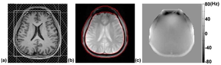
CSI experiment with 130 ms TE and lipid suppression: (a) positions of the excitation volume and OVS bands; (b) anatomical image overlaid with the boundaries of the support of the lipid signal; and (c) measured field map.
Experiment II: Hybrid CSI/EPSI scan with only water suppression
A hybrid CSI/EPSI dataset was acquired with only water suppression from the same subject immediately after Experiment I. The excitation region of the CSI scan was 200 × 200 mm2; no OVS bands were used for lipid suppression. The other imaging parameters of the CSI scan were the same as in Experiment I. A PRESS-EPSI sequence was used to acquire high-resolution spectroscopic data to help remove the strong lipid signal leakage in the CSI data. The EPSI scan had the same water suppression, FOV, excitation volume and TR/TE as the CSI scan. The rest of imaging parameters of the EPSI data were: 80 × 80 spatial encodings, 100kHz readout bandwidth, bipolar readout, number of echoes = 120, echo space = 1.03 ms. The data acquisition time of the EPSI scan was 2.1 min.
Experiment III: SPICE with water and lipid suppression
Another hybrid CSI/EPSI dataset was collected to reconstruct high-resolution spectroscopic data using the SPICE method (25) and to demonstrate nuisance signal removal in acquisitions with sparse sampling of (k, t)-space. The imaging parameters of the CSI data were: 240 × 240 mm2 FOV, 160 × 150 mm2 excitation region, 10mm slice thickness, TR/TE = 1600/130 ms, 12 × 12 spatial encodings, 2000 Hz readout bandwidth, WET pulses for water suppression and eight OVS bands for lipid suppression. The data acquisition time of the CSI scan was 3.8 min. The EPSI data were collected with the same water and lipid suppression setup, FOV, excitation volume and TR/TE as the CSI data, as well as the following parameters: 80 × 80 spatial encodings (3 mm in-plane resolution), 100 kHz readout bandwidth, bipolar readout, number of echoes = 120, echo space = 1.03 ms, 12 averages. The data acquisition time of the EPSI scan was 26.4 min. The GRE sequence in Experiment I was used to acquire a field map. Two spin-echo (SE) images were acquired with 1200/30 ms and 1200/130 ms TR/TE, respectively, to obtain high-resolution structural information for SPICE. The other imaging parameters of the two SE images were: 240 × 240 mm2 FOV, 128 × 128 spatial encodings, and 2.6 min data acquisition.
Data processing
Prior to nuisance signal removal, two processing steps are needed to correct for eddy-currents and data misalignment.
Eddy-currents can cause time shift and phase mismatch between the odd and even echoes of the EPSI acquisition, resulting in aliasing artifacts in the reconstructed spectrum. To correct this mismatch, two navigator signals were acquired without phase-encoding blips. The readout gradients for the first navigator signal were the same as in the EPSI readout, while the second the opposite in amplitude. The average time shift was estimated by calculating the correlation functions of the odd and even echoes (after data reordering) using the first navigator data. Then, the average phase mismatch was estimated by comparing the phase difference between the echoes of the first and second navigator data (after data reordering and time shift correction). We used the estimated time shift and constant and linear phase difference to correct the eddy-current effects on the EPSI data.
The spatial misalignment between the CSI and EPSI data was also determined and corrected. The CSI data was first zero-padded to the same matrix size as the EPSI data, and The Fourier reconstructions of the two datasets were then obtained. Two integral images were calculated by taking spectral integrals of the magnitudes of the Fourier reconstructions such that the correlation matrix of the two images determined the spatial misalignment. The zero-padded CSI reconstruction was shifted accordingly, transformed back to (k, t)-space, and truncated to obtained the alignment-corrected CSI data.
The nuisances signals were removed from conventional CSI or hybrid CSI/EPSI data using the proposed method. For comparison, the extrapolation method in (14) was implemented using the Papoulis-Gerchberg (PG) algorithm, and is referred to as the PG method throughout this work. In the PG method, the spectroscopic data was extrapolated to a 64 × 64 grid. For both methods, the collected multi-channel raw data were processed channel by channel. The nuisance signal removed, multi-channel data were then combined using the method in (45). Additionally, we reconstructed high-resolution metabolite signals from the SPICE acquisition with nuisance signals removed. For more details of the SPICE method, please refer to Ref. (25). The performance of the proposed method was illustrated using representative spectra and N-acetyl aspartate (NAA) maps. The NAA maps were generated by taking the integral of the magnitude of the nuisance signal removed spectra in a range of 2.02 ± 0.1ppm. No baseline correction was used as the baseline signals were negligible in the presented long-TE (130 ms) MRSI data.
Results
Experiment I: CSI scan with water and lipid suppression
The method presented in Case 1 of the Theory section was used to remove the lipid signal (residuals after suppression) from the CSI data, and was compared with the PG method. Results are shown in Fig. 2. The NAA map of the original data shows noticeable ringing artifacts from the subcutaneous lipid layer. These ringing artifacts are significantly reduced in the PG reconstruction; however, there is noticeable signal loss near the boundary of the brain, a known issue of the PG method (14, 18). In contrast, the NAA map obtained by the proposed method shows no noticeable ringing artifacts and better metabolite signal protection near the boundary of the brain. Representative spectra before and after lipid signal removal are shown in the second to the forth columns of Fig. 2. Remaining lipid signals are found in the spectra obtained by the PG method, especially near the subcutaneous lipid layer, while the spectra obtained by the proposed method show “lipid-free” metabolite signals.
Figure 2.
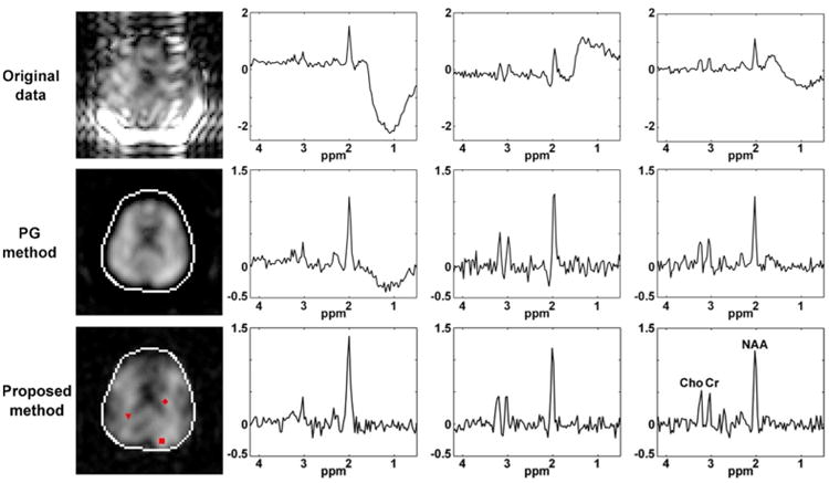
The method presented in Case 1 of the Theory section was used to remove the lipid signal (residuals after suppression) from the CSI data in Experiment I, and was compared with the PG method. The first column shows the NAA maps calculated using the original data, the PG reconstruction, and the reconstruction using the proposed method, respectively. In the PG reconstruction, the signal in the subcutaneous lipid layer is masked out for better display. The boundary of the brain is overlaid. The top and bottom images are zero-padded for comparison with the PG method. The second to the forth column show the corresponding spectra of each method, indicated by the box, triangle and diamond, respectively.
Experiment II: Hybrid CSI/EPSI scan with only water suppression
The method presented in Case 3 of the Theory section was used to remove the residual water signal and the lipid signal from the hybrid CSI/EPSI dataset. The PG method was used to remove the lipid signal from CSI data for comparison. Results are shown in Fig. 3 and 4. To illustrate the performance of the proposed method, while assuming the sampling along the readout direction of the EPSI sequence be instantaneous, a Fourier transform was used to reconstruct MRSI images from the original EPSI data, the estimated residual water signal (resampled along the sampling trajectory of the EPSI sequence), the estimated lipid signal (resampled along the sampling trajectory of the EPSI sequence) and the nuisance signal removed data. Spectral integrals of these reconstructions are shown in Fig. 3a to 3d, respectively. The estimated residual water signal in Fig. 3b indicates that the water suppression was effective except in the regions with large field inhomogeneities (see the field map in Fig. 1c). After the nuisance signals were removed, the residual signal in Fig. 3d only shows noise due to the very low SNR of the EPSI data, but also indicates successful nuisance signal removal using the proposed method. Representative spectra of the estimated lipid and the estimated residual water signal are shown in Fig. 3e and 3f. Note that the peak around 5.8 ppm in Fig. 3e and the peak around 8 ppm Fig. 3f are the spectral aliasing artifacts caused by direct Fourier transform reconstruction.
Figure 3.
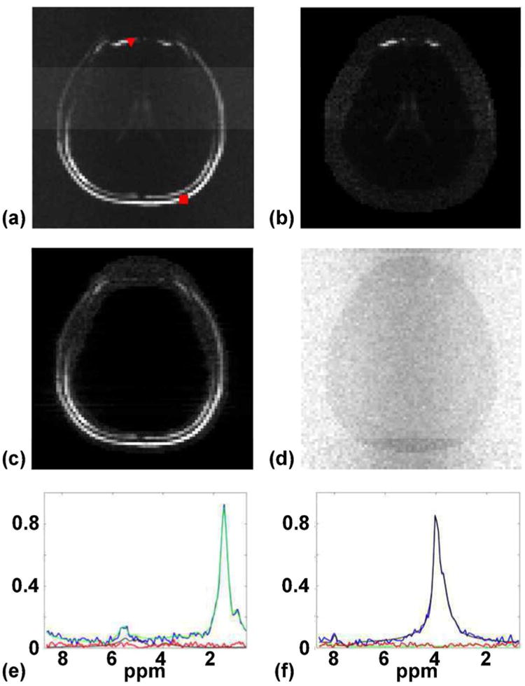
The method presented in Case 3 of the Theory section was used to remove the residual water signal and the lipid signal from the EPSI dataset in Experiment II. Spectral integrals of the original EPSI data, the estimated residual water signal, the estimated lipid signal and the nuisance signal removed data are shown in (a) to (d), respectively. Representative spectra of the estimated lipid signal (the box in (a)) and the estimated residual water signal (the triangle in (a)) are shown in (e) and (f), respectively (blue line: original signal; green line: estimated lipid signal; black line: estimated residual water signal; and red line: residuals).
Figure 4.
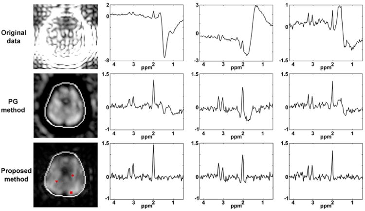
The method presented in Case 3 of the Theory section was used to remove the lipid signal from the CSI dataset in Experiment II. The results are arranged as in Fig. 2, comparing the original data with lipid removal using the PG method and the proposed method. Despite the significant corruption due to lack of lipid suppression, the proposed method sufficiently recovers the spectra of the metabolite signals.
Lipid removal results of the CSI data with only water suppression are shown in Fig. 4. Severe leakage of the lipid signals is seen in the NAA map of the original CSI data (the first row of Fig. 4), and there are significant lipid signals left in the PG reconstruction (the second row of Fig. 4). There are no noticeable lipid signals in the spectra obtained by the proposed method (the last row of Fig. 4).
Figure 5 shows an example of rank selection in the proposed method. The red lines in Fig. 5a to 5c show the singular value distributions (in decibel) of the Casorati matrices formed from the residual water signal, the lipid signal and the metabolite signal, respectively, using the CSI data acquired with only water suppression. The black dashed line in Fig. 5 shows the singular value distribution of a random Gaussian matrix formed based on the measured noise variance. We chose the rank of each component so that the next singular value would be smaller than the largest singular value of the random matrix. In this specific example, the chosen rank of the residual water signal, the lipid signal and the metabolite signal was 15, 9, and 3, respectively.
Figure 5.
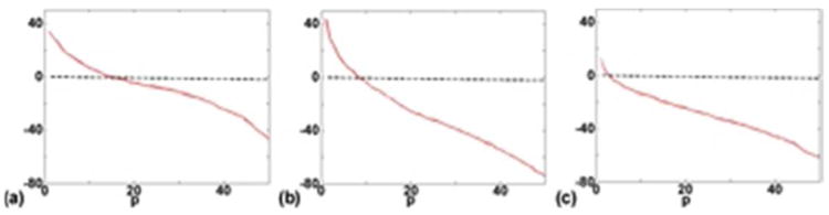
Rank selection. Using the CSI data in Experiment II, Casorati matrices of the the residual water signal, the lipid signal, and the metabolite signal were formed. The corresponding singular value distributions (in decibel) are shown in (a) to (c). The black dashed line shows the singular value distribution of a random Gaussian matrix formed based on the measured noise variance, which served as the cutoff for temporal basis selection in the proposed method. The singular values were normalized to the largest singular value of the Gaussian random matrix.
Figure 6 shows the effects of the discrepancies in magnitude and phase between the CSI and EPSI data when the high-resolution lipid signal estimated from the EPSI data was used to remove the lipid signal from the low-resolution CSI data. If these discrepancies were ignored and the lipid signal estimated from the EPSI data was directly used to remove the lipid signal from the CSI data by truncation in (k, t)-space, significant residual lipid signals would be found in the resulting CSI data, as shown in Fig. 6a and 6b. In the proposed method, the discrepancies were corrected using a GS model and the residual lipid signals were effectively reduced as shown in Fig. 6c and 6d.
Figure 6.
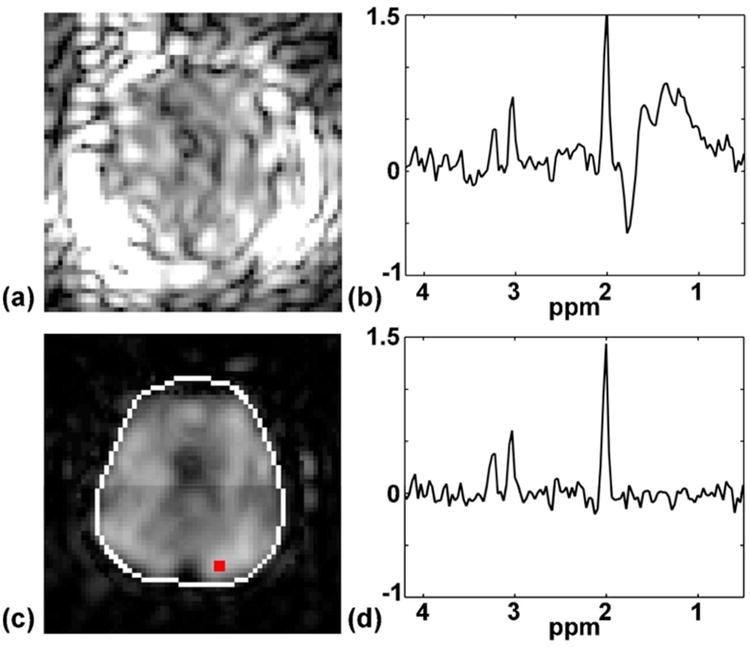
Effects of the magnitude and phase discrepancies between the CSI and EPSI data on nuisance signal removal. Using the hybrid CSI/EPSI data acquired without lipid suppression, the high-resolution lipid signal estimated from the EPSI data was directly used to remove the lipid signal from the CSI data by truncation in (k,t)-space. The resulting NAA map and a representative spectrum are shown in (a) and (b), where residuals of the lipid signal are dominant. However, if the discrepancies between the CSI and EPSI data are corrected, as in the proposed method, the remaining lipid signals are significantly reduced ((c) and (d)).
Experiment III: SPICE with water and lipid suppression
The method presented in Case 3 of the Theory section was used to remove the water and lipid signals (residuals after suppression) from the SPICE data. Figure 7 shows the results of nuisance signal removal in SPICE. The Fourier transform reconstructions of the original EPSI data and the estimated water and lipid signals were obtained, and the spectral integrals of the magnitude of the reconstructions are shown in Fig. 7a to 7c. NAA maps were calculated using the nuisance-signal removed EPSI and CSI data and were zero-padded to a 80 × 80 grid for display (corresponding the resolution of the original EPSI data). Especially, the EPSI data was truncated to a 32 × 32 grid in k-space to gain SNR before calculating its NAA map. As expected, the NAA map of the EPSI data (Fig. 7d) has very low SNR even after truncation in k-space. The NAA map of the CSI data (Fig. 7e) has low resolution but high SNR. More importantly, Fig. 7d and 7e show that the proposed method successfully removed the nuisance signals from the EPSI and CSI data, making it possible to use SPICE for high-resolution spectroscopic imaging. Indeed, the NAA map of the SPICE reconstruction (Fig. 7f) has both high spatial and spectral resolution, along with high SNR. The spectra of the SPICE reconstruction have SNR nearly comparable to those of the CSI reconstruction, as shown in Fig. 7g and 7h. Note that the lateral ventricle structure of the brain, which is known to have low NAA concentration levels, is clearly seen in the SPICE reconstruction.
Figure 7.
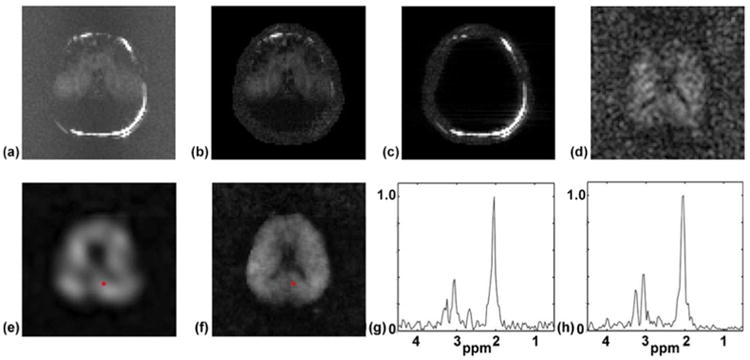
Nuisance signal removal in SPICE using the method presented in Case 3 of the Theory section. Spectral integrals of the original EPSI data, the estimated residual water signal and the estimated residual lipid signal are shown in (a) to (c), respectively. NAA maps calculated using the nuisance-signal removed EPSI and CSI data, and the SPICE reconstruction are shown in (d) to (f), respectively. Both the CSI and EPSI reconstructions were free of nuisance signals, as was the SPICE reconstruction. Representative spectra of the CSI and SPICE reconstruction are shown in (g) and (h).
Discussion
The proposed union-of-subspaces model provides a general framework for nuisance signal removal in 1H MRSI, which leverages the PS properties and the prior knowledge of the spatialspectral supports of the nuisance and metabolite signals. Our in vivo experiment results show that the proposed method can effectively remove the nuisance signals from MRSI data with limited and/or sparse (k, t)-space coverage. The resulting spectra were almost free of lipid contamination, even when no lipid suppression was used during data acquisition.
In the case of conventional MRSI with limited k-space coverage, the proposed method better removes the lipid signal than the extrapolation method (14–16), which only uses the spatial support of the lipid signal, as shown in Fig. 2. If the MRSI data are severely corrupted by the lipid signal, e.g., in MRSI without lipid suppression or at short TE, high-resolution (k, t)-space data can be acquired in a short auxiliary scan using fast MRSI sequences to help remove the lipid signal as shown in Fig.3 and Fig. 4. This data acquisition scheme has been used in the dual-density method (20–24). Compared to the dual-density method, the proposed method can shorten the auxiliary scan by allowing sparse sampling of the high-resolution (k, t)-space data and gains robustness by using the GS model to compensate the discrepancies between the high-resolution and low-resolution data.
In the case of sparse (k, t)-space data, the proposed method can effectively remove both the water and lipid signals. This is desirable for accelerated MRSI techniques that reconstruct high-resolution spectroscopic data from sparsely sampled (k, t)-space data by exploiting the prior knowledge of the underlying metabolite signal, such as sparsity (26, 27) and PS (25). In this work, we show a case where the proposed method was used to remove the nuisance signals from sparsely sampled (k, t)-space data followed by the recently proposed SPICE method (25) to reconstruct high-resolution spectroscopic data with high SNR (Fig. 7). The SPICE method exploits the PS properties of the metabolite signal, and thus the dominant water and lipid signals need to be removed prior to reconstruction.
The proposed method can be further optimized for practical applications. First, it is critical to accurately estimate the temporal basis of each signal component from limited k-space data that are corrupted by magnetic field inhomogeneities. In this article, we use the CP method to correct the magnetic field inhomogeneity effects. Additional prior knowledge and constraints can be incorporated for more accurate subspace estimation. This issue is under investigation and will be addressed in a subsequent paper. Second, advanced regularization schemes can be used to better estimate the spatial coefficients in Eq. [6]. For example, weighted-ℓ2 regularization can be used to incorporate prior knowledge of edges and ℓ1 regularization can be used to promote the sparsity of the nuisance and metabolite signals.
Conclusions
We have presented a new union-of-subspaces approach for nuisance signal removal from proton MRSI data. In vivo experiment results have shown that the proposed method can effectively remove nuisance signals from limited and/or sparse (k, t)-space data. The proposed method may prove useful for MRSI of the brain, especially for accelerated high-resolution MRSI with sparse sampling of (k, t)-space.
Acknowledgments
Grant sponsor: National Institutes of Health; Grant number: 1R01-EB013695; Grant sponsor: Beckman Postdoctoral Fellowship (to Chao Ma)
References
- 1.Haase A, Frahm J, Hanicke W, Matthaei D. 1H NMR chemical shift selective (CHESS) imaging. Phys Med Biol. 1985;30:341–344. doi: 10.1088/0031-9155/30/4/008. [DOI] [PubMed] [Google Scholar]
- 2.Ogg RJ, Kingsley PB, Taylor JS. WET, a T1- and B1-insensitive water-suppression method for in vivo localized 1H NMR spectroscopy. J Magn Reson Series B. 1994;104:1–10. doi: 10.1006/jmrb.1994.1048. [DOI] [PubMed] [Google Scholar]
- 3.Tkac I, Starcuk Z, Choi IY, Gruetter R. In vivo 1H NMR spectroscopy of rat brain at 1 ms echo time. Magn Reson Med. 1999;41:649–656. doi: 10.1002/(sici)1522-2594(199904)41:4<649::aid-mrm2>3.0.co;2-g. [DOI] [PubMed] [Google Scholar]
- 4.de Graaf RA, Nicolay K. Adaibatic water suppression using frequency selective excitation. Magn Reson Med. 1998;40:690–696. doi: 10.1002/mrm.1910400508. [DOI] [PubMed] [Google Scholar]
- 5.Luo Y, de Graaf RA, DelaBarre L, Tannus A, Garwood M. BISTRO: An outer-volume suppression method that tolerates RF field inhomogeneity. Magn Reson Med. 2001;45:1095–1102. doi: 10.1002/mrm.1144. [DOI] [PubMed] [Google Scholar]
- 6.Duyn JH, Gillen J, Sobering G, van Zijl PCM, Moonen CTW. Multisection proton MR spectroscopic imaging of the brain. Radiology. 1993;188:277–282. doi: 10.1148/radiology.188.1.8511313. [DOI] [PubMed] [Google Scholar]
- 7.Le Roux P, Gilles RJ, McKinnon GC, Carlier PG. Optimized outer volume suppression for single-shot fast spin-echo cardiac imaging. J Magn Reson Imaging. 1998;8:1022–1032. doi: 10.1002/jmri.1880080505. [DOI] [PubMed] [Google Scholar]
- 8.Spielman D, Pauly JM, Macovski A, Glover GH, Enzmann DR. Lipid-suppressed single- and multisection proton spectroscopic imaging of the human brain. J Magn Reson Imaging. 1992;2:253–262. doi: 10.1002/jmri.1880020302. [DOI] [PubMed] [Google Scholar]
- 9.Ebel A, Govindaraju V, Maudsley AA. Comparison of inversion recovery preparation schemes for lipid suppression in 1H MRSI of human brain. Magn Reson Med. 2003;49:903–908. doi: 10.1002/mrm.10444. [DOI] [PubMed] [Google Scholar]
- 10.Spielman D, Pauly J, Macovski A, Enzmann D. Spectroscopic imaging with multidimensional pulses for excitation: SIMPLE. Magn Reson Med. 1991;19:67–84. doi: 10.1002/mrm.1910190107. [DOI] [PubMed] [Google Scholar]
- 11.Andronesi OC, Gagoski BA, Sorensen AG. Neurologic 3D MR spectroscopic imaging with low-power adiabatic pulses and fat spiral acquisition. Radiology. 2012;262:647–661. doi: 10.1148/radiol.11110277. [DOI] [PMC free article] [PubMed] [Google Scholar]
- 12.Brown TR, Kincaid BM, Ugurbil K. NMR chemical shift imaging in three dimensions. Proc Natl Acad Sci USA. 1982;79:3523–3526. doi: 10.1073/pnas.79.11.3523. [DOI] [PMC free article] [PubMed] [Google Scholar]
- 13.Barkhuysen H, de Beer R, van Ormondt D. Improved algorithm for noniterative time-domain model fitting to exponentially damped magnetic resonance signals. J Magn Reson. 1987;73:553–557. [Google Scholar]
- 14.Haupt CI, Schuff N, Weiner MW, Maudsley AA. Removal of lipid artifacts in 1H spectroscopic imaging by data extrapolation. Magn Reson Med. 1996;35:678–687. doi: 10.1002/mrm.1910350509. [DOI] [PMC free article] [PubMed] [Google Scholar]
- 15.Pelvritis SK, Macovski A. MRS imaging using anatomically based k-space sampling and extrapolation. Magn Reson Med. 1995;34:686–693. doi: 10.1002/mrm.1910340506. [DOI] [PubMed] [Google Scholar]
- 16.Pelvritis SK, Macovski A. Spectral extrapolation of spatially bounded images. IEEE Trans Med Imaging. 1995;14:487–497. doi: 10.1109/42.414614. [DOI] [PubMed] [Google Scholar]
- 17.Dong Z, Hwang JH. Lipid signal extraction by SLIM: Application to 1H MR spectroscopic imaging of human calf muscles. Magn Reson Med. 2006;55:1447–1453. doi: 10.1002/mrm.20895. [DOI] [PubMed] [Google Scholar]
- 18.Hernando D, Haldar J, Sutton B, Liang ZP. Removal of lipid signal in MRSI using spatial-spectral constraints. IEEE International Symposium on Biomedical Imaging, USA. 2007:1360–1363. [Google Scholar]
- 19.Hernando D, Haldar J, Sutton B, Liang ZP. Removal of lipid nuisance signals in MRSI using spatial-spectral constraints. Proc of the International Symposium on Magnetic Resonance in Medicine, Germany. 2007:1244. [Google Scholar]
- 20.Bligic B, Gagioski B, Kok T, Adalsteinsson E. Lipid suppression in CSI with spatial priors and highly undersampled peripheral k-space. Magn Reson Med. 2013;69:1501–1511. doi: 10.1002/mrm.24399. [DOI] [PMC free article] [PubMed] [Google Scholar]
- 21.Hu X, Patel M, Ugurbil K. A new strategy for spectroscopic imaging. J Magn Reson Series B. 1994;36:21–29. doi: 10.1006/jmrb.1994.1004. [DOI] [PubMed] [Google Scholar]
- 22.Hu X, Patel M, Chen W, Ugurbil K. Reduction of truncation artifacts in chemical-shift imaging by extended sampling using variable repetition time. J Magn Reson Series B. 1995;106:292–296. doi: 10.1006/jmrb.1995.1047. [DOI] [PubMed] [Google Scholar]
- 23.Metzger G, Sarkar S, Zhang X, Heberlein K, Patel M, Hu X. A hybrid technique for spectroscopic imaging with reduced truncation artifact. Magn Reson Imaging. 1999;17:435–443. doi: 10.1016/s0730-725x(98)00187-8. [DOI] [PubMed] [Google Scholar]
- 24.Sarkar S, Heberlein K, Hu X. Truncation artifact reduction in spectroscopic imaging using a dual-density spiral k-space trajectory. Magn Reson Imaging. 2002;20:743–757. doi: 10.1016/s0730-725x(02)00608-2. [DOI] [PubMed] [Google Scholar]
- 25.Lam F, Liang ZP. A subspace approach to high-resolution spectroscopic imaging. Magn Reson Med. 2014;71:1349–1357. doi: 10.1002/mrm.25168. [DOI] [PMC free article] [PubMed] [Google Scholar]
- 26.Chatnuntawech I, Gagoski B, Bilgic B, Cauley SF, Setsompop K, Adalsteinsson E. Accelerated 1H MRSI using randomly undersampled spiral-based k-space trajectories. Magn Reson Med. doi: 10.1002/mrm.25394. [DOI] [PubMed] [Google Scholar]
- 27.Cao P, Wu Ex. Accelerating phase-encoded proton MR spectroscopic imaging by compressed sensing. J Magn Recon Med. doi: 10.1002/jmri.24553. [DOI] [PubMed] [Google Scholar]
- 28.Liang ZP. Spatiotemporal imaging with partially separable functions. IEEE International Symposium on Biomedical Imaging, USA. 2007:988–991. [Google Scholar]
- 29.Haldar JP, Liang ZP. Spatiotemporal imaging with partially separable functions: A matrix recovery approach. IEEE International Symposium on Biomedical Imaging, Netherlands. 2010:716–719. [Google Scholar]
- 30.Nguyen HM, Peng X, Do MN, Liang ZP. Denoising MR spectroscopic imaging data with low-rank approximations. IEEE Trans BioMed Eng. 2013;60:78–89. doi: 10.1109/TBME.2012.2223466. [DOI] [PMC free article] [PubMed] [Google Scholar]
- 31.Posse S, Tedeschi G, Risinger R, Ogg R, Bihan DL. High speed 1H spectroscopic imaging in human brain by echo planar spatial-spectral encoding. Magn Reson Med. 1995;33:34–40. doi: 10.1002/mrm.1910330106. [DOI] [PubMed] [Google Scholar]
- 32.Ma C, Lam F, Johnson CL, Liang ZP. Removal of nuisance lipid signals from limited k-space data in 1H MRSI of the brain. Proc of the International Symposium on Magnetic Resonance in Medicine, Italy. 2014:2887. [Google Scholar]
- 33.Lu YM, Do MN. A theory for sampling signals from a union of subspaces. IEEE Trans Signal Processing. 2008;56:2334–2345. [Google Scholar]
- 34.de Graaf RA. In vivo NMR spectroscopy. 2nd. New York: Wiley; 2007. [Google Scholar]
- 35.Brix G, Heiland S, Bellemann ME, Koch T, Lorenz WJ. MR imaging of fat containing tissues: valuation of two quantitative imaging techniques in comparison with localized proton spectroscopy. Magn Reson Imaging. 1993;11:977–991. doi: 10.1016/0730-725x(93)90217-2. [DOI] [PubMed] [Google Scholar]
- 36.Macovski A. Volumetric NMR imaging with time-varying gradients. Magn Reson Med. 1985;2:29–40. doi: 10.1002/mrm.1910020105. [DOI] [PubMed] [Google Scholar]
- 37.Noll DC, Fessler JA, Sutton BP. Conjugate phase MRI reconstruction with spatially variant sample density correction. IEEE Trans Med Imaging. 2005;24:325–336. doi: 10.1109/tmi.2004.842452. [DOI] [PubMed] [Google Scholar]
- 38.Marchenko VA, Pastur LA. Distribution of eigenvalues for some sets of random matrices. Math USSR Sb. 1967;1:457–483. [Google Scholar]
- 39.Haldar JP, Hernando D, Song SK, Liang ZP. Anatomically constrained reconstruction from noisy data. Magn Reson Med. 2008;59:810–818. doi: 10.1002/mrm.21536. [DOI] [PubMed] [Google Scholar]
- 40.Vogel CR. Computational methods for inverse problems. Philadelphia, PA: SIAM; 2002. [Google Scholar]
- 41.Hernando D, Kellman P, Haldar JP, Liang ZP. Robust water/fat separation in the presence of large field inhomogeneities using a graph-cut algorithm. Magn Reson Med. 2010;63:79–90. doi: 10.1002/mrm.22177. [DOI] [PMC free article] [PubMed] [Google Scholar]
- 42.Liang ZP, Lauterbur PC. An efficient method for dynamic magnetic resonance imaging. IEEE Trans Med Imaging. 1994;13:677–686. doi: 10.1109/42.363100. [DOI] [PubMed] [Google Scholar]
- 43.Liang ZP, Lauterbur PC. A generalized series approach to MR spectroscopic imaging. IEEE Trans Med Imaging. 1991;10:132–137. doi: 10.1109/42.79470. [DOI] [PubMed] [Google Scholar]
- 44.Ordidge RJ, Bendall MR, Gordon RE, Connelly A. Volume selection for in vivo biological spectroscopy. In: Govil G, Khetrapal CL, Saran A, editors. Magnetic resonance in biology and medicine. New Delhi: Tata McGraw-Hill Publishing Company Ltd; 1985. pp. 387–397. [Google Scholar]
- 45.Bydder M, Hamilton G, Yokoo T, Sirlin CB. Optimal phased-array combination for spectroscopy. Magn Reson Imaging. 2008;26:847–850. doi: 10.1016/j.mri.2008.01.050. [DOI] [PMC free article] [PubMed] [Google Scholar]