Pleistocene megafaunal interaction networks became more vulnerable after human arrival

Abstract

The end of the Pleistocene was marked by the extinction of almost all large land mammals worldwide except in Africa. Although the debate on Pleistocene extinctions has focused on the roles of climate change and humans, the impact of perturbations depends on properties of ecological communities, such as species composition and the organization of ecological interactions. Here, we combined palaeoecological and ecological data, food-web models and community stability analysis to investigate if differences between Pleistocene and modern mammalian assemblages help us understand why the megafauna died out in the Americas while persisting in Africa. We show Pleistocene and modern assemblages share similar network topology, but differences in richness and body size distributions made Pleistocene communities significantly more vulnerable to the effects of human arrival. The structural changes promoted by humans in Pleistocene networks would have increased the likelihood of unstable dynamics, which may favour extinction cascades in communities facing extrinsic perturbations. Our findings suggest that the basic aspects of the organization of ecological communities may have played an important role in major extinction events in the past. Knowledge of community-level properties and their consequences to dynamics may be critical to understand past and future extinctions.

1. Introduction

The end of the Pleistocene was marked by an extinction event (the late Quaternary extinction, LQE) that led to the demise of large vertebrates, affecting the organization of ecosystems worldwide [1,2]. The greatest impact was on the mammalian megafauna (more than or equal to 44 kg) with the extinction of more than 100 genera [2,3]. The LQE was particularly severe in Australia and the Americas where more than 70% of the megafauna genera perished [2]. Africa retains the remnants of these, once widespread, large-mammal assemblages (including megaherbivores with body mass more than 1000 kg; [4]). The debate on the main causes of the LQE is not settled [2]. Most studies on the Pleistocene extinctions focus on external triggers for the extinctions [5,6], such as direct [1,7] and indirect [2,8] impacts of humans, climate change [9] and combinations thereof [3,10]. However, both empirical and theoretical work support the notion that community organization, as determined by species composition and ecological interactions, dictates how perturbations propagate through the ecological community, determining the fate of populations [11–13]. Therefore, the answer for why megafauna died out almost everywhere except Africa could reside not only in the perturbations themselves, but also in the intrinsic properties of Pleistocene large-mammal assemblages.

Theory predicts that basic features of ecological systems have large effects on the way perturbations propagate [14]. Specifically, species richness, the number and strength of interactions and the way interactions are distributed among species affect if population densities within a community will re-establish (stability) or diverge (instability) after a perturbation [15–17]. Although unstable communities are not necessarily destined to collapse, if communities are unstable or populations take too long to re-establish, fluctuations may reduce populations to critically low densities, making them vulnerable to demographic stochasticity and local extinction [18]. Therefore, rather than an absolute description of how vulnerable an ecological community is or was, examining the stability of ecological communities with different structural properties provides a comparative assessment of the vulnerability of different systems to perturbations. Qualitative stability analysis provides a theoretical framework to infer how the organization of ecological communities affects stability [14–19]. Despite the simplifying assumptions of qualitative stability analysis, this approach predicts different aspects of empirical ecological communities [20–22], including empirical sequences of extinctions, bringing insights on the disassembly of ecological communities [23].

Here, we combine palaeontological and ecological data, food-web models, stability analysis, and extinction and introduction simulations to explore the role of species interactions in shaping the dynamics of past and present assemblages of large mammals. Despite the insights brought about by indirect evidence of interactions [24] and methods such as isotope analysis [25], determining who interacted with whom in palaeoecological communities is challenging [13]. To account for the uncertainty inherent to any characterization of ecological networks, we used body mass information and a probabilistic network model [23,26] (figure 1) to generate an ensemble of potential predator–prey networks depicting interactions among Pleistocene large mammals in the Americas (electronic supplementary material, table S1). After cross-validating the reconstructed networks with palaeoecological data (electronic supplementary material, Appendix S1), we investigated the topology of reconstructed networks and used local stability analysis [15,17] to examine whether differences in the organization of species interactions offer insights on why large-mammal assemblages collapsed in North and South America, but persisted in Africa. Finally, to understand possible effects of human arrival to the Americas, we tested how the invasion by a new predator would impact community dynamics in different locations by altering community organization.

Figure 1.

Reconstructing predator–prey interactions. (a) Conceptual representation of the model [26] used to reconstruct predator–prey interaction networks. The model assumes body mass relationships determine the probability of interactions between predators and prey, as depicted by the probability curves corresponding to each predator (according to colour coding and position). (b) Example of a probability matrix produced by a model run parametrized with the information for an assemblage from Africa. Colour heat illustrates the probability of each interaction between predators (rows) and prey (columns). The matrix is ordered by body size. This model correctly reproduced on average 75% of the interactions within the three predator–prey systems from modern Africa analysed.

2. Material and methods

(a). Large-mammal assemblages

We searched the literature and the Paleobiology Database (http://paleobiodb.org/; accessed May 2013) for Pleistocene fossil assemblages for which the composition, chronology and taphonomy suggest an actual community of interacting species. We avoided sites with a mammalian fauna that seemed too incomplete based on our knowledge of Pleistocene faunas more generally, or those with dates that were too unconstrained, which would have yielded time-averaged assemblages. We ended up with five Late Pleistocene sites in North America and four sites in South America (electronic supplementary material, table S1 and data S1). Because we are interested in interactions among large mammals, we established systematic criteria to determine which species to consider. We considered only mammalian herbivores larger than 5 kg, which are more likely to be preyed upon by the carnivores that make up the large mode of the body size distribution [27,28]. Accordingly, we only included carnivore species larger than 10 kg. In this way, we avoided including carnivores such as small felids, which rely mainly on rodents and other small prey and probably played a minor role in the predator–prey dynamics of large mammalian assemblages. Therefore, we considered here only the large-mammal assemblages within communities, which form cohesive compartments in the food webs [29]. Although these species may be involved in multiple types of interactions such as cooperative interactions in mixed herds or intraguild predation, we focus here on the trophic interactions between carnivores and herbivores.

We obtained information on the body mass of Pleistocene mammals from compiled data available in the literature [30]. When no body mass estimate was available for a given species, we used the average body mass of species within the same genus. For the comparisons with modern systems, we used three mammalian assemblages from Africa for which we have information on observed predator–prey interactions (electronic supplementary material, table S1).

(b). Reconstructing predator–prey interaction networks

Here, we adopt the reasonable assumption that ancient and extant large-mammal assemblages are organized by similar processes [4]. Thus, a model that is able to reproduce interaction patterns between African large mammals should be appropriate to reconstruct Pleistocene networks with a realistic structure. Because body mass is often considered a key trait in determining species interactions [31], including predator–prey interactions between terrestrial mammals [27,28,32], we parametrized network models using species body mass. Therefore, prior to the reconstruction of Pleistocene networks, we used data on the interactions between large-mammals in three locations in Africa (electronic supplementary material, table S1) to test the performance of two different models—the probabilistic niche model (PNM) and the log ratio model (LRM)—in reproducing observed large-mammal interaction patterns. Because the performance of the LRM was better than that of the PNM (see Results), we used only the LRM to reconstruct Pleistocene networks. For information on the PNM, see electronic supplementary material, appendix S2.

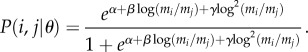
The LRM is a statistical model that uses the log ratio of the body mass of predator and prey species as the explanatory variable [26]. The probability of interactions can be modelled as a logit regression:

2.1

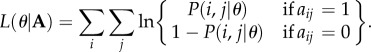
in which a_ij is a cell in the binary matrix A that depicts species interactions; a_ij = 1, if there is an interaction between predator i and prey j and zero otherwise, and α, β and γ are parameters to be estimated. The model has a quadratic polynomial term and, hence, the interaction probabilities form a Gaussian-like curve reflecting the idea of an optimal range for the predator. This formulation is consistent with other food-web models based on the niche concept such as the PNM [33]. Thus, the probability of an interaction between predator i and prey j given a particular parameter set θ = {α, β, γ} is

2.2

For both models (the LRM and PNM), different parameter sets result in different probabilities of interaction. The maximum-likelihood parameter set is that which maximizes the log-likelihood:

2.3

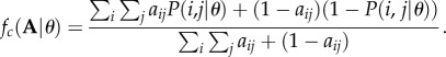
We combined the simulated annealing optimization and the Latin hypercube sampling technique to find the parameter set that maximizes the likelihood of each model; see Pires & Guimarães [34] for a similar approach. To compare model performance, we used the Akaike information criterion (AIC). The model with the lowest relative value of AIC is the one showing the best fit to the data. To provide a straightforward characterization of the performance of the models in reproducing each predator–prey network between African large mammals, we also computed the fraction of presences and absences of pairwise interactions (1's and 0's in matrix A) each model correctly predicts when parametrized with the maximum-likelihood estimates:

2.4

Previous studies using network models parametrized with body mass information showed body size alone is unable to predict interaction patterns of several species in food webs [26,35]. However, when focusing on smaller ‘subnetworks', with only two trophic levels and fewer groups, as we did here, the performance of the models is greatly improved (see Results). A good fit of models parametrized only with body mass to a whole food web would indicate body size translates into interaction patterns in a similar way for different groups and different trophic levels, which seems unlikely. By contrast, our dataset includes only large mammalian predators, all carnivorans, and prey, mostly ungulates. It is reasonable to assume that this smaller set of species obey similar rules regarding how body size relationships map into interaction patterns.

To generate Pleistocene predator–prey networks representing each site, we first defined the range of the three parameters α, β and γ of the LRM. The extremes of the range of each parameter were the smallest and largest values found as MLEs for the three African sites. By doing so, we adopt the assumption that the constraints imposed on diet by the body mass relationship between predator and prey were similar in Pleistocene and modern African large-mammal communities [36]. Although we used the parameters estimated for the African networks, the parameters only determine how the probability of interactions is linked to body mass relationships. The number of predator and prey species and body mass distribution in each assemblage are the factors that determine network organization. To generate a network, we then sampled values of α, β and γ within the defined range and computed all p_ij to obtain a matrix P. Each matrix P was then used to generate a binary matrix, A, depicting interactions among predator and prey species in each assemblage. Because this procedure envisages incorporating the uncertainty inherent to inferring interactions among extinct species, we generated 10⁵ possible interaction networks for each site.

To cross-validate our procedure for reconstructing Pleistocene networks, we searched the literature for evidence of predator–prey interactions between the species considered here. We considered studies using different methods such as isotope analyses, indirect evidence of predation, reconstructions based on biomechanical constraints and palaeontological knowledge, and studies on interactions among surviving species (electronic supplementary material, appendix S1).

(c). Network topology

To characterize network topology, we focused on two topological properties: nestedness [37] and modularity [38]. Nestedness and modularity describe how interaction patterns overlap and are related to community dynamics [39]. Nestedness is high when the interactions of species with few interaction partners form a subset of the interactions of more connected species [40]. We used the metric NODF [37] to compute the degree of nestedness of each predator–prey network built using the model. NODF tends to 100 for highly nested networks and to zero when species show other non-random patterns of interaction [37].

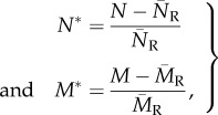
Network modularity is high when the network has groups (modules) of highly connected species that are loosely connected to other species in the network [38]. To find the partition of a given network that maximizes within-module interactions relative to between-module interactions, we used a simulated annealing optimization algorithm implemented in the program MODULAR [41]. We computed modularity using a modularity index, herein M, designed specifically for bipartite networks [42]. M tends to 0 when between-module interactions largely exceed within-module interaction, and increases towards 1 when the network contains completely isolated modules. Because the number of species and interactions affects both NODF [37] and M [38], we computed the relative nestedness and modularity to allow comparisons across different networks [40]:

2.5

where N and M are the nestedness and modularity degrees of each network generated by the model, and N̄_R and M̄_R are the average nestedness and modularity of random networks with the same number of species and same average number of interactions, where all interactions are equiprobable [40]. With this null model approach, we are not aiming to test the significance of topological patterns, but to control for the statistical effects of connectance and species richness on these metrics so we are able to compare different assemblages.

(d). The community matrix and local stability analysis

To analyse the dynamical behaviour of large-mammal assemblages, we assume system dynamics can be approximated by a unspecified predator–prey model, where predators have a negative impact on prey populations, prey have a positive impact on predator populations and all populations are subject to density-dependent regulation. Under such a model, competition between predators is also implicitly included since predators affect each other indirectly by reducing the densities of shared prey.

Starting from each binary matrix A_{m × n}, we built an adjacency matrix Q of size S × S, where S is the total number of species (m + n). Each matrix cell, q_ij, represents the effect of individuals of species i on the population of species j (interaction strength) around a feasible equilibrium [17]. Thus, Q can be viewed as an approximation to the Jacobian matrix [17] and, therefore, the dynamics of the potential communities under a small perturbation, such as fluctuations in population densities, are given by the real part of the leading eigenvalue, λ_ℝ, of Q [17]. We computed the proportion of matrices with stable behaviour, λ_ℝ < 0, as a measure of the probability that communities are stable, P_st. For matrices presenting stable behaviour, we also computed the average time to return to equilibrium, τ ∼ 1/|λ_ℝ| [18]. To compute confidence intervals, we repeated analyses 100 times for each site.

Interaction strengths depend on the per capita effect of interactions and abundances of interacting species, but the specific way interaction strengths are estimated depends on the underlying dynamic model considered [43]. In the baseline analyses, we do not make any particular assumption on functional responses, so, instead of estimating interaction strengths from model parameters, we assigned values drawn from probability distributions [17] (see electronic supplementary material, appendix S2, for further details on building Q). This approach allowed us to investigate how the combination of species composition and network topology of each site would affect dynamics without constraints of particular dynamic model assumptions. We then tested which characteristics of the assemblages were the most important in determining stability (electronic supplementary material, appendix S2). The main drawback of studying dynamics without assuming a particular model is that we cannot evaluate the feasibility of the analysed equilibrium points [44]. To address this issue, we replicated the analyses assuming a Lotka–Volterra model and examined the stability of feasible equilibrium points alone [43] (see electronic supplementary material, appendix S2).

Stability analysis only allows us to examine how a dynamical system at equilibrium behaves after small perturbations. However, despite its limited scope, stability analysis provides a comprehensive way to bridge structure and dynamics, since under this framework stability ultimately depends on the likelihood that the effects of perturbations spread across the elements of the system through their interactions [14]. The usefulness in connecting structure and dynamics is the reason for the ubiquity of stability analysis in the study of ecological systems [14,16,18,23].

(e). Removal simulations

Unstable communities are not necessarily destined to collapse. A system may reach alternative states with different stability properties after rearranging. To find how changes in the species composition of a given site would impact community dynamics, we performed simulations removing species and recalculating the eigenvalues for the resulting community matrices. Starting from 100 community matrices per site, we removed species combined in groups of size k (1 ≤ k ≤ S − 1) and registered the change in λ_ℝ. When the number of combinations for a given k exceeded 10⁵, we tested 10⁵ random combinations, otherwise we tested all possible combinations of species. We then registered the smallest change in species richness (measured as the difference in richness before and after removals) that resulted in the largest reduction in λ_ℝ relative to the original matrix. By doing this, we searched for assemblages that were stable, highly resilient, but retained a large number of species. We also registered the species composition that yielded the smallest λ_ℝ possible, i.e. the richness of predator and prey species that maximize resilience for each assemblage.

(f). The impact of human arrival on dynamics

To infer how the arrival of humans in the Americas would have affected community dynamics, we tested the impact of an additional predator on P_st. Archaeological evidence suggests Late Pleistocene hunters were able to take down prey much larger than would be expected based on human average body size [45–47]. Hence, we simulated humans assuming their interaction patterns would be similar to those of large-sized predators such as Smilodon (average body mass: 250 kg). This assumption is supported by archaeological evidence [46]. Because humans may have actively exterminated large predators, we also tested the effect of humans on stability while considering humans had negative direct effects over other predators (see electronic supplementary material, appendix S2, for further details).

The effects of humans may be due to their ability to feed on prey of different sizes or just because the networks are vulnerable to the addition of any predator. To control for the effect adding a predator could have on stability, we measured the effect of adding a small-sized predator (30 kg). We computed the effects of humans on stability as: where and are the probabilities of stability after and before the additions.

3. Results

To reconstruct Pleistocene predator–prey networks, we first tested the performance of two probabilistic network models (PNM and LRM) parametrized with body mass information in reproducing networks depicting interactions between African large mammals. Using only the number of predator and prey species and their average body mass as input parameters, the models were able to predict on average more than 70% of the interactions correctly (LRM: f_c = 0.83, 0.68, 0.74; PNM: f_c = , 0.76, 0.70, 0.77; for the Kruger, Mala Mala and Serengeti datasets). The LRM had the best fit (lower AIC) for two of the three African networks (LRM: AIC = 68.82, 76.32, 72.30; PNM: AIC = 90.88, 85.74, 71.40) and was used to reconstruct the Pleistocene networks. These reconstructions using body mass relationships often yielded assemblages where large predators have broad and overlapping diets and smaller predators consume mainly the smallest herbivores in each site (electronic supplementary material, figure S1). These interaction patterns are consistent with those obtained from palaeoecological inferences using other methods such as isotope analyses or based on inferences from biomechanics and ecomorphology (electronic supplementary material, appendix S1). Thus, these models allowed us to reconstruct realistic interaction networks while encompassing the uncertainty of which interactions would have occurred in the past, as well as their expected variation across space and time, instead of assuming a single network topology.

We then focused on the structure of the reconstructed Pleistocene predator–prey networks and whether the composition of Pleistocene mammalian assemblages would be more likely to generate unstable dynamics when compared to modern mammalian assemblages in Africa. Using corrected indices, which control for variation in species richness and network connectance, we found no trend suggesting that the degree of nestedness or modularity of Pleistocene assemblages would be consistently higher or lower than those of modern African assemblages (figure 2a; electronic supplementary material, table S2). If we consider the absolute degrees of nestedness and modularity, high nestedness and low modularity characterized both Pleistocene and African large-mammal networks (electronic supplementary material, figure S2 and table S2). High nestedness means the resource use patterns of predators overlap asymmetrically and low modularity indicates predators cannot be grouped according to their prey preferences.

Figure 2.

The topology and dynamics of large-mammal assemblages. (a) The average (±s.d.) degree of relative nestedness (NODF*) and relative modularity (M*) of reconstructed Pleistocene predator–prey networks. The limits of the yellow rectangle define the range of values for modern African assemblages. Panel (b,c) depicts the effect of basic community properties on stability. Partial regression plots show the probability of stability of communities, P_st, as a function of predator richness (b) and the average body mass of prey (c) after controlling for all other variables. Different colours represent the assemblages from different continents, as coded in the map. Values for the y- and x-axes in (b,c) were standardized by removing the effects of the other variables in the regression model. Test statistics in electronic supplementary material, table S5.

High nestedness and low modularity are often associated with lower stability in predator–prey interactions [39]. Analysing the dynamics of large-mammal assemblages, we found that Pleistocene assemblages were as prone to being unstable as modern African assemblages. The values of probability of stability, P_st, and average time to return to equilibrium, τ, estimated for the African assemblages were within the range of values computed for Pleistocene assemblages (electronic supplementary material, tables S3 and S4). Multiple regression analyses (electronic supplementary material, appendix S2) showed that both P_st (F_2,9 = 53.63; R² = 0.90; p < 0.001) and τ (F_2,9 = 68.85; R² = 0.92; p < 0.001) were well predicted by basic characteristics of each assemblage (electronic supplementary material, tables S5 and S6). Lower P_st (figure 2; electronic supplementary material, table S5) and higher τ (electronic supplementary material, table S6) values were mainly associated with larger predator-richness and lower average body mass of prey species. These results hold if matrices are built under different assumptions, such as random interaction strengths, body-mass-driven interaction strengths or considering asymmetries in the magnitude of the effect of interactions for predators and prey (see electronic supplementary material, appendix S2 and tables S3–S6). We also found the main feature of the assemblages determining the probability of stability was predator richness when we assumed a Lotka–Volterra model and examined only feasible equilibrium points (electronic supplementary material, figure S3 and tables S5 and S6).

By simulating extinctions and looking at the dynamics of the resulting assemblages, we also found that assemblages with fewer predators (electronic supplementary material, figure S4) were more likely to be stable and more resilient (smaller τ values). Yet, for all sites, stable assemblages with the greatest resilience to small perturbations were simplified assemblages with low species richness, similar to present-day large-mammal assemblages in the Americas (electronic supplementary material, figure S5). Although these assemblages are more resilient when facing small perturbations, they show no redundancy and are thus extremely vulnerable to species loss.

We next looked at the impacts of human arrival on the dynamics of Pleistocene assemblages. We simulated humans as generalist predators capable of preying upon medium- and large-sized prey. Faunal assemblages with humans present were invariably more prone to instability and had longer return times than original communities, as expected from the destabilizing effects of increasing predator richness (figure 2). Although humans were already part of the food web in Pleistocene Africa, African assemblages can be used as a benchmark to assess the magnitude of the effect of humans on stability. Thus, we performed the same analysis on African assemblages for comparison. We found the arrival of humans should affect assemblages similar to modern African assemblages and Pleistocene assemblages in distinct ways. In the three African assemblages, the effects of humans on the probability of stability would be similar to the effect of adding a small predator (figure 3). Conversely, in American Pleistocene assemblages, the destabilizing effect of humans would be considerably larger (figure 3). Results are similar if we consider extinct Pleistocene African mammals as part of the African assemblages (electronic supplementary material, appendix S2, table S7 and figure S6). When we considered the possibility that humans directly impacted other predator populations, the destabilizing effects of added humans were greater, but the effects on modern assemblages were still smaller than on the Pleistocene assemblages (electronic supplementary material, figure S7).

Figure 3.

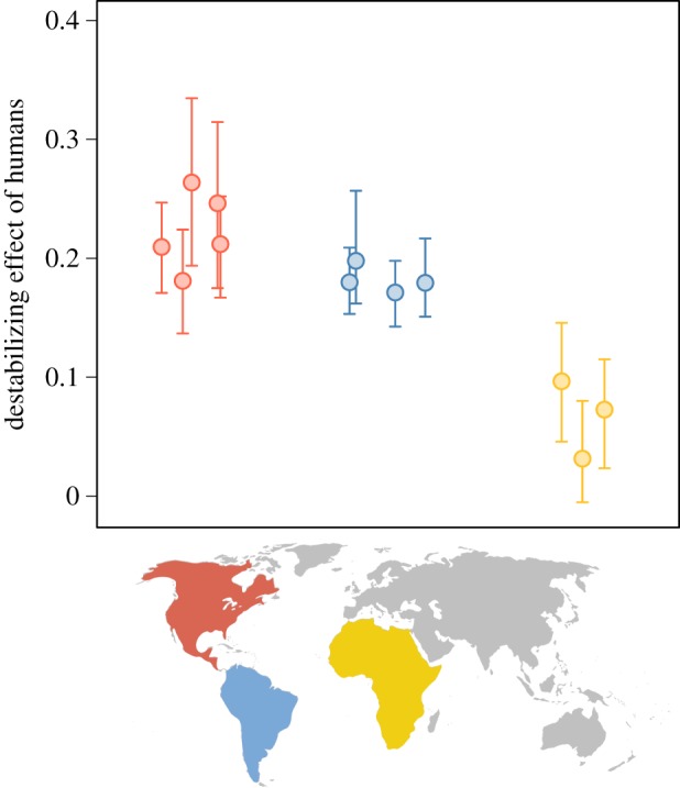
The impact of human arrival on community stability. Each point represents the destabilizing effect of humans in a given site. Assemblages from different continents are grouped by the position in the x-axis and colours, as coded in the map. Error bars depict the 95% CI. Values close to zero mean the destabilizing effect of humans would not be greater than the expected effect of an additional small-sized predator.

4. Discussion

Our results suggest Pleistocene large-mammal assemblages were not intrinsically prone to be unstable when compared to modern African communities, but were more sensitive to the arrival of a large predator such as humans. Taken together, our findings reveal three important aspects of Pleistocene large-mammal assemblages likely to have contributed to shape Pleistocene extinction patterns.

First, we show how differences in the composition of large-mammal assemblages affect their response to perturbations. Large predators often have large dietary breadths and may interact strongly with many species [27,32]. By contrast, megaherbivores escape predation from most predators, interacting only weakly with the largest predators [32], and are controlled mainly by bottom-up processes [27]. As a consequence, large predators and large prey have opposite roles in community structure: large predators increase connectivity and have greater per capita interaction strength, whereas large herbivores contribute to a less connected community with weak interactions. Increased connectivity and stronger interactions reduce the stability of ecological communities [14,15,17]. Thus, the likelihood that the effects of a perturbation will spread throughout the community should be larger in a community with many large predators, but smaller in communities with many large herbivores. In our dataset, the average number of predator species is greater in North American than in South American Pleistocene sites. In general, Pleistocene faunas in North America had richer predator assemblages, whereas South American faunas had richer large-herbivore assemblages [6,48,49]. Although dates for Pleistocene fossils from South America are still sparse compared to North America, existing information indicates that the LQE took longer in South America than it did in North America [45,50]. Our findings suggest that the high diversity of large herbivores and the relatively lower diversity of predators might have favoured stability in South American assemblages. Stability analysis is not intended to predict the long-term outcomes of perturbations. Thus, lower probability of stability does not necessarily imply in higher likelihood of collapse. Yet, these intrinsic differences in stability could have interacted with external factors such as differences in the timing of human arrival [51], to generate the chronology of megafaunal extinctions in the Americas.

Second, our results from extinction simulations suggest simplified communities with smaller richness of both predator and prey species would be resilient. This result agrees with the general theoretical understanding that simpler systems are easier to attain stable dynamics than species-rich communities [15]. The simplified assemblages resulting from removal simulations are similar to present-day assemblages in the Americas. The richest modern large-mammal assemblages in the Americas, such as those in the Yellowstone Park or central South America [52,53], have no more than three large predators and half a dozen prey species, which is probably close to the Early Holocene scenario after the LQE. Even though our results suggest impoverished assemblages are more resilient to small perturbations than their Pleistocene counterparts, low diversity implies a lack of functional redundancy [23], which is often linked to increased vulnerability to extinction cascades [11,29]. We hypothesize that the composition of present-day large-mammal assemblages in the Americas is the consequence of rearrangements that resulted in communities resilient to small perturbations, such as small variations in population densities. However, such rearranged communities are so species-poor that they became highly vulnerable to species loss [23].

Third, we found the effects of humans should be greater in American Pleistocene assemblages than in Late Pleistocene or modern African assemblages. It has been argued that large mammals in Africa were less vulnerable to hunting because they coevolved with humans for millions of years [1]. Alternatively, modern African assemblages may represent assemblages that were rearranged in response to human influence at an earlier stage [1]. Both processes are candidate explanations for the differences in vulnerability to human impact we observed between African and American assemblages. Late Pleistocene assemblages in the Americas had more large herbivores than the African assemblages. Our analyses on the determinants of dynamics suggest that, in the absence of humans, large herbivores promote stability in large-mammal assemblages. However, human arrival would have shifted the effects of large herbivores on stability. Humans did not necessarily have to consume large amounts of all prey to have an impact on dynamics. By interacting with a broad range of prey, including the large herbivores, humans would greatly increase the connectivity and the proportion of strong interactions in Pleistocene assemblages, thus changing their network structure and dynamics in ways that made them more susceptible to the effects of perturbations. Here, we only simulated humans as generalized predators. This approach is a first step in understanding how humans could have altered the dynamics of Pleistocene interaction networks. However, more complex hunting behaviours could generate different patterns of interactions, thus affecting dynamics in different ways. For instance, although we focus here on predator–prey networks, recent work show the stability of food webs is hindered by highly connected species feeding on multiple levels [54]. As humans are capable of exploiting resources from different trophic levels in the food web, we hypothesize that destabilizing consequences of human arrival may have affected other subsets of Pleistocene communities.

We analysed dynamics under a framework, which, as any modelling approach, asks for simplifying assumptions. We acknowledge that factors not included in the models such as spatial heterogeneity or different mechanisms of interaction switches over time could produce unanticipated outcomes and decouple persistence and local stability by buffering the effects of perturbations. Yet, our approach allowed us to examine potential differences and similarities in the dynamics of ancient and modern large-mammal assemblages and bring more elements of community ecology to the debate. Future work should focus on evaluating the generality of our results by adapting other promising modelling approaches, such as adaptive network dynamics [55], Boolean networks [56] and structural stability analysis [44], to the study of predator–prey interactions. These additional approaches may allow the consideration of other layers of biological information and the investigation of the robustness of our findings.

Our results contribute to our understanding of Pleistocene extinctions by probing into the network organization and dynamics of Pleistocene assemblages. There is compelling archaeological evidence that humans hunted large Pleistocene herbivores in the Americas [45–47], but debate continues about whether human overhunting was the main driver of megafaunal extinction [2,7], or if other factors contributed to the LQE. Our results suggest humans, as predators that were able to exploit a variety of prey in Pleistocene communities, would have promoted structural changes in these systems, reducing the likelihood of stability, which in turn may favour extinction cascades and reduce species persistence when facing other extrinsic perturbations such as habitat alteration or climate change. Moreover, our findings have implications that go beyond the study of Pleistocene systems as they reveal that knowledge of basic aspects of community structure and the network organization of species interactions may be important to understand past and future large extinction events. Such insights are increasingly important given the prevalence of human impact on contemporary faunas.

Data accessibility

The datasets supporting this article have been uploaded as part of the electronic supplementary material.

Authors' contributions

M.M.P., P.L.K. and P.R.G. designed research. M.M.P., P.L.K. and R.A.F. compiled the dataset. M.M.P., P.R.G., P.L.K., M.A.M.A. and S.F.R. contributed to analysis design. M.M.P. performed analyses. All authors contributed to the discussion of results. M.M.P. and P.R.G. wrote the paper and all authors contributed to the final draft.

Competing interests

We declare we have no competing interests.

Funding

Work was supported with grant nos. 2006/04682-5, 2009/54422-8 and 2009/54567-6, São Paulo Research Foundation (FAPESP).

References

- 1.Martin PS, Klein RG. 1984. Quaternary extinctions: a prehistoric revolution. Tucson, AZ: University of Arizona Press. [Google Scholar]
- 2.Koch PL, Barnosky AD. 2006. Late Quaternary extinctions: state of the debate. Annu. Rev. Ecol. Evol. Syst. 37, 215–250. ( 10.1146/Annurev.Ecolsys.34.011802.132415) [DOI] [Google Scholar]
- 3.Barnosky AD. 2008. Megafauna biomass tradeoff as a driver of Quaternary and future extinctions. Proc. Natl Acad. Sci. USA 105, 11 543–11 548. ( 10.1073/pnas.0801918105) [DOI] [PMC free article] [PubMed] [Google Scholar]
- 4.Owen-Smith N. 1987. Pleistocene extinctions—the pivotal role of megaherbivores. Paleobiology 13, 351–362. [Google Scholar]
- 5.Scott E. 2010. Extinctions, scenarios, and assumptions: changes in latest Pleistocene large herbivore abundance and distribution in western North America. Q. Int. 217, 225–239. ( 10.1016/J.Quaint.2009.11.003) [DOI] [Google Scholar]
- 6.Fariña RA, Vizcaíno SF, De Iuliis G, Tambusso S. 2013. Megafauna: giant beasts of Pleistocene South America (life of the past). Bloomington, IL: Indiana University Press. [Google Scholar]
- 7.Alroy J. 2001. A multispecies overkill simulation of the end-Pleistocene megafaunal mass extinction. Science 293, 1893–1896. ( 10.1126/science.1059342) [DOI] [PubMed] [Google Scholar]
- 8.Barnosky AD, Koch PL, Feranec RS, Wing SL, Shabel AB. 2004. Assessing the causes of Late Pleistocene extinctions on the continents. Science 306, 70–75. ( 10.1126/science.1101476) [DOI] [PubMed] [Google Scholar]
- 9.Guthrie RD. 1984. Mosaics, allelochemicals, and nutrients: an ecological theory of Late Pleistocene megafaunal extinctions. In Quaternary extinctions: a prehistoric revolution (eds Martin PS, Klein RG), pp. 259–298. Tucson, AZ: University of Arizona Press. [Google Scholar]
- 10.Prescott GW, Williams DR, Balmford A, Green RE, Manica A. 2012. Quantitative global analysis of the role of climate and people in explaining late Quaternary megafaunal extinctions. Proc. Natl Acad. Sci. USA 109, 4527–4531. ( 10.1073/Pnas.1113875109) [DOI] [PMC free article] [PubMed] [Google Scholar]
- 11.Estes JA, et al. 2011. Trophic downgrading of planet Earth. Science 333, 301–306. ( 10.1126/Science.1205106) [DOI] [PubMed] [Google Scholar]
- 12.Forster MA. 2003. Self-organised instability and megafaunal extinctions in Australia. Oikos 103, 235–239. ( 10.1034/j.1600.0706.2003.12557.x) [DOI] [Google Scholar]
- 13.Roopnarine PD. 2006. Extinction cascades and catastrophe in ancient food webs. Paleobiology 32, 1–19. ( 10.1666/05008.1) [DOI] [Google Scholar]
- 14.Rooney N, McCann KS. 2012. Integrating food web diversity, structure and stability. Trends Ecol. Evol. 27, 40–46. ( 10.1016/J.Tree.2011.09.001) [DOI] [PubMed] [Google Scholar]
- 15.May RM. 1972. Will a large complex system be stable? Nature 238, 413–414. ( 10.1038/238413a0) [DOI] [PubMed] [Google Scholar]
- 16.Neutel AM, Heesterbeek JAP, van de Koppel J, Hoenderboom G, Vos A, Kaldeway C, Berendse F, de Ruiter PC. 2007. Reconciling complexity with stability in naturally assembling food webs. Nature 449, 599–602. ( 10.1038/Nature06154) [DOI] [PubMed] [Google Scholar]
- 17.Allesina S, Tang S. 2012. Stability criteria for complex ecosystems. Nature 483, 205–208. ( 10.1038/Nature10832) [DOI] [PubMed] [Google Scholar]
- 18.Loeuille N. 2010. Influence of evolution on the stability of ecological communities. Ecol. Lett. 13, 1536–1545. ( 10.1111/J.1461.0248.2010.01545.X) [DOI] [PubMed] [Google Scholar]
- 19.Pimm SL. 2002. Food webs. Chicago, IL: University of Chicago Press. [Google Scholar]
- 20.Gross T, Rudolf L, Levin SA, Dieckmann U. 2009. Generalized models reveal stabilizing factors in food webs. Science 325, 747–750. ( 10.1126/science.1173536) [DOI] [PubMed] [Google Scholar]
- 21.Yodzis P. 1981. The stability of real ecosystems. Nature 289, 674–676. ( 10.1038/289674a0) [DOI] [Google Scholar]
- 22.de Ruiter PC, Neutel A-M, Moore JC. 1995. Energetics, patterns of interaction strengths, and stability in real ecosystems. Science 269, 1257–1260. ( 10.1126/science.269.5228.1257) [DOI] [PubMed] [Google Scholar]
- 23.Yeakel JD, Pires MM, Rudolf M, Dominy NJ, Koch PL, Guimarães PR, Gross T. 2014. Collapse of an ecological network in Ancient Egypt. Proc. Natl Acad. Sci. USA 111, 14 472–14 477. ( 10.1073/pnas.1408471111) [DOI] [PMC free article] [PubMed] [Google Scholar]
- 24.Marean CW, Ehrhardt CL. 1995. Paleoanthropological and paleoecological implications of the taphonomy of a sabertooth's den. J. Hum. Evol. 29, 515–547. ( 10.1006/jhev.1995.1074) [DOI] [Google Scholar]
- 25.Yeakel J, Guimarães PR, Bocherens H, Koch PL. 2013. The impact of climate change on the structure of Pleistocene food webs across the mammoth steppe. Proc. R. Soc. B 280, 20130239 ( 10.1098/rspb.2013.0239) [DOI] [PMC free article] [PubMed] [Google Scholar]
- 26.Rohr RP, Scherer H, Kehrli P, Mazza C, Bersier LF. 2010. Modeling food webs: exploring unexplained structure using latent traits. Am. Nat. 176, 170–177. ( 10.1086/653667) [DOI] [PubMed] [Google Scholar]
- 27.Owen-Smith N, Mills MGL. 2008. Predator–prey size relationships in an African large-mammal food web. J. Anim. Ecol. 77, 173–183. ( 10.1111/J.1365-2656.2007.01314.X) [DOI] [PubMed] [Google Scholar]
- 28.Carbone C, Mace GM, Roberts SC, Macdonald DW. 1999. Energetic constraints on the diet of terrestrial carnivores. Nature 402, 286–288. ( 10.1038/46607) [DOI] [PubMed] [Google Scholar]
- 29.Terborgh J, Estes JA. 2010. Trophic cascades: predators, prey, and the changing dynamics of nature. Washington, DC: Island Press. [Google Scholar]
- 30.Smith FA, Lyons SK, Ernest SKM, Jones KE, Kaufman DM, Dayan T, Marquet PA, Brown JH, Haskell JP. 2003. Body mass of late Quaternary mammals. Ecology 84, 3403 ( 10.1890/02-9003) [DOI] [Google Scholar]
- 31.Brose U. 2010. Body-mass constraints on foraging behaviour determine population and food-web dynamics. Funct. Ecol. 24, 28–34. ( 10.1111/J.1365-2435.2009.01618.X) [DOI] [Google Scholar]
- 32.Sinclair ARE, Mduma S, Brashares JS. 2003. Patterns of predation in a diverse predator–prey system. Nature 425, 288–290. ( 10.1038/nature01934) [DOI] [PubMed] [Google Scholar]
- 33.Williams RJ, Purves DW. 2011. The probabilistic niche model reveals substantial variation in the niche structure of empirical food webs. Ecology 92, 1849–1857. ( 10.1890/11-0200.1) [DOI] [PubMed] [Google Scholar]
- 34.Pires MM, Guimarães PR. 2013. Interaction intimacy organizes networks of antagonistic interactions in different ways. J. R. Soc. Interface 10, 20120649 ( 10.1098/rsif.2012.0649) [DOI] [PMC free article] [PubMed] [Google Scholar]
- 35.Williams RJ, Anandanadesan A, Purves D. 2010. The probabilistic niche model reveals the niche structure and role of body size in a complex food web. PLoS ONE 5, e12092 ( 10.1371/journal.pone.0012092) [DOI] [PMC free article] [PubMed] [Google Scholar]
- 36.Prevosti FJ, Vizcaíno SF. 2006. Paleoecology of the large carnivore guild from the Late Pleistocene of Argentina. Acta Palaeontol. Pol. 51, 407–422. [Google Scholar]
- 37.Almeida-Neto M, Guimarães P, Guimarães PR, Loyola RD, Ulrich W. 2008. A consistent metric for nestedness analysis in ecological systems: reconciling concept and measurement. Oikos 117, 1227–1239. ( 10.1111/j.0030-1299.2008.16644.x) [DOI] [Google Scholar]
- 38.Olesen JM, Bascompte J, Dupont YL, Jordano P. 2007. The modularity of pollination networks. Proc. Natl Acad. Sci. USA 104, 19 891–19 896. ( 10.1073/pnas.0706375104) [DOI] [PMC free article] [PubMed] [Google Scholar]
- 39.Thébault E, Fontaine C. 2010. Stability of ecological communities and the architecture of mutualistic and trophic networks. Science 329, 853–856. ( 10.1126/science.1188321) [DOI] [PubMed] [Google Scholar]
- 40.Bascompte J, Jordano P, Melián CJ, Olesen JM. 2003. The nested assembly of plant–animal mutualistic networks. Proc. Natl Acad. Sci. USA 100, 9383–9387. ( 10.1073/pnas.1633576100) [DOI] [PMC free article] [PubMed] [Google Scholar]
- 41.Marquitti FMD, Guimarães PR, Pires MM, Bittencourt LF. 2014. MODULAR: software for the autonomous computation of modularity in large network sets. Ecography 37, 221–224. ( 10.1111/j.1600.0587.2013.00506.x) [DOI] [Google Scholar]
- 42.Barber MJ. 2007. Modularity and community detection in bipartite networks. Phys. Rev. E 76, e0066102 ( 10.1103/PhysRevE.76.066102) [DOI] [PubMed] [Google Scholar]
- 43.Emmerson M, Yearsley JM. 2004. Weak interactions, omnivory and emergent food-web properties. Proc. R. Soc. Lond. B 271, 397–405. ( 10.1098/rspb.2003.2592) [DOI] [PMC free article] [PubMed] [Google Scholar]
- 44.Rohr RP, Saavedra S, Bascompte J. 2014. On the structural stability of mutualistic systems. Science 345, 1–9. ( 10.1126/science.1253497) [DOI] [PubMed] [Google Scholar]
- 45.Cione AL, Tonni EP, Soibelzon L. 2009. Did humans cause the Late Pleistocene–Early Holocene mammalian extinctions in South America in a context of shrinking open areas? In American megafaunal extinctions at the end of the Pleistocene (ed. Haynes G.), pp. 125–144. Dordrecht, The Netherlands: Springer. [Google Scholar]
- 46.Surovell TA, Waguespack NM. 2008. How many elephant kills are 14? Clovis mammoth and mastodon kills in context. Q. Int. 191, 82–97. ( 10.1016/j.quaint.2007.12.001) [DOI] [Google Scholar]
- 47.Fariña RA, Tambusso P, Varela L, Czerwonogora A, Di Giacomo M, Musso M, Bracco-Boksar R, Gascue A. 2014. Arroyo del Vizcaíno, Uruguay: a fossil-rich 30-ka-old megafaunal locality with cut-marked bones. Proc. R. Soc. B 281, 20132211 ( 10.1098/rspb.2013.2211) [DOI] [PMC free article] [PubMed] [Google Scholar]
- 48.Lyons SK, Smith FA, Brown JH. 2004. Of mice, mastodons and men: human-mediated extinctions on four continents. Evol. Ecol. Res. 6, 339–358. [Google Scholar]
- 49.Fariña RA. 1996. Trophic relationships among Lujanian mammals. Evol. Theory 11, 125–134. [Google Scholar]
- 50.Barnosky AD, Lindsey EL. 2010. Timing of Quaternary megafaunal extinction in South America in relation to human arrival and climate change. Q. Int. 217, 10–29. ( 10.1016/j.quaint.2009.11.017) [DOI] [Google Scholar]
- 51.Sandom C, Faurby S, Sandel B, Svenning J-C. 2014. Global late Quaternary megafauna extinctions linked to humans, not climate change. Proc. R. Soc. B 281, 20133254 ( 10.1098/rspb.2013.3254) [DOI] [PMC free article] [PubMed] [Google Scholar]
- 52.Smith DW, Peterson RO, Houston DB. 2003. Yellowstone after wolves. Bioscience 53, 330–340. ( 10.1641/0006-3568) [DOI] [Google Scholar]
- 53.Crawshaw PG, Quigley HB. 2002. Jaguar and puma feeding habits in the Pantanal, Brazil, with implications for their management and conservation. In El jaguar en el nuevo milenio (eds Medellin RA, Equihua C, Chetkiewicz C), pp. 223–235. New York, NY: Wildlife Conservation Society. [Google Scholar]
- 54.Johnson S, Domínguez-García V, Donetti L, Muñoz MA. 2014. Trophic coherence determines food-web stability. Proc. Natl Acad. Sci. USA 111, 17 923–17 928. ( 10.1073/pnas.1409077111) [DOI] [PMC free article] [PubMed] [Google Scholar]
- 55.Gross T, Sayama H. 2009. Adaptive networks: theory, models and applications. New York, NY: Springer. [Google Scholar]
- 56.Campbell C, Yang S, Albert R, Shea K. 2011. A network model for plant–pollinator community assembly. Proc. Natl Acad. Sci. USA 108, 197–202. ( 10.1073/pnas.1008204108) [DOI] [PMC free article] [PubMed] [Google Scholar]
Associated Data
This section collects any data citations, data availability statements, or supplementary materials included in this article.
Supplementary Materials
Data Availability Statement