Confidence Interval of the Likelihood Ratio Associated with Mixed Stain DNA Evidence

Abstract

Likelihood ratios are necessary to properly interpret mixed stain DNA evidence. They can flexibly consider alternate hypotheses and can account for population substructure. The likelihood ratio should be seen as an estimate and not a fixed value, because the calculations are functions of allelic frequency estimates that were estimated from a small portion of the population. Current methods do not account for uncertainty in the likelihood ratio estimates and are therefore an incomplete picture of the strength of the evidence. We propose the use of a confidence interval to report the consequent variation of likelihood ratios. The confidence interval is calculated using the standard forensic likelihood ratio formulae and a variance estimate derived using the Taylor expansion. The formula is explained, and a computer program has been made available. Numeric work shows that the evidential strength of DNA profiles decreases as the variation among populations increases.

With techniques for obtaining and typing DNA evidence becoming more sensitive, the need for interpreting mixed stains is growing. Unfortunately, analysis of DNA mixtures is both genetically and statistically complex (1), and care is needed not to present prejudicial analyses. Several lines of research have been explored to simplify the mixture analysis process. Peak areas in chromatograms have been considered to help resolve mixtures (2,3), and denaturing high-performance liquid chromatography has been used to resolve mitochondrial mixtures (4). The majority of mixture evidence comes from sexual assault cases, and much work has been devoted to analysis of the Y chromosome to identify male perpetrators (5).

While much progress has been made in typing methods, the development of statistical methods has been slower. Weir et al. (6) gave a general formulation under the assumption of allelic independence, and this was extended by Curran et al. (7) to allow for population structure. The case of mixed race populations has been examined (8), and Lauritzen and Mortera (9) provided a useful bound for the number of unknown contributors to a mixture.

One statistical topic that has not received much attention is that of the effects of sampling variation on the numbers presented for DNA mixtures. For single-contributor stains, methods to describe the effects of sampling variation have been reviewed by Curran et al. (10) and by Gill et al. (11). This paper proposes the reporting of likelihood ratios for DNA mixtures and presents an analytical method that can be, and has been, incorporated into a software package.

The Confidence Interval

It has become accepted practice to attach numerical weights to DNA evidence to show “whether the patterns are as common as pictures with two eyes, or as unique as the Mona Lisa” (US v Yee, 134 FRD 161, 181 [ND Ohio, 1991]). Probability assessments should accurately inform the court of the strength of the evidence. However, a simple quantification of probability does not tell the whole story. Calculations for mixtures, as for single-contributor stains, rest on the frequencies of alleles at the typed markers yet these frequencies are not known. Instead, they are estimated using a sample from the population. Because these samples represent only a small portion of the total population, there is uncertainty about the true frequencies and therefore uncertainty about the resulting calculations. If the forensic scientist wishes to report on the evidence accurately and thoroughly, the level of uncertainty should in some way be reported. Some investigators (12–14) advocate the use of Bayesian methods that lead to probability distributions of mixture quantities, and there is merit to that approach. However, deciding on an appropriate prior in the context of an adversarial court setting may prove difficult.

Here, we present the classical approach of confidence intervals, in part because they avoid the need for controversial priors, and in part because they are familiar in the context of public opinion surveys (“47% of those polled support the President on this issue, plus or minus 3 percentage points”). It is understood that the “plus or minus” results from the estimated proportion depending on the particular set of people sampled. We do not mean to imply that forensic scientists should adopt statistical procedures only because they can be explained easily, but we point out that the widely used confidence interval is a statistical tool with a rigorous theoretical basis.

Technically, a confidence interval refers to the range in which a specified central proportion (say 95%) of future estimates would fall if further samples were taken from the population and each one used to provide an estimate. Presenting a confidence interval is the appropriate response to the question “How large a sample is necessary to provide an estimate?” The forensic scientist can explain that the sample size used resulted in a certain width confidence interval. Smaller samples would widen the interval, and larger samples would make it narrower. It is worth noting that the common phrase “plus or minus 3 percentage points” generally reflects the uncertainty in the proportion of a population responding to one answer to a single question when 1000 or so people are questioned. For DNA profiles to match, there is a question (“is there a match?”) that must be answered correctly for each allele in the evidence profile, and the resulting confidence interval is more likely to be “plus or minus a factor of 3.”

The definition of a confidence interval leads naturally to the technique of bootstrapping, whereby a new sample is created by resampling the sample at hand (15). If 1000 new samples are created in this way, and the 1000 new estimates are put in rank order, then a 95% confidence interval is bounded by the 26th and the 975th estimates. While bootstrapping makes few distributional assumptions, other than the original sample being appropriately random, bootstrapping from a single population cannot address the evolutionary sampling implicit in forensic calculations that employ the “theta correction.” The approach we employ for both single- and multiple-contributor stains supposes that allele frequencies are not necessarily available from the most relevant population or subpopulation, but that the available frequencies can be used, along with the population structure parameter θ, in a way that recognizes the variation among populations caused by evolutionary processes.

We offer, therefore, an algebraic treatment that employs sample allele frequencies and a specified value of θ. Access to the original database is not needed, although a computer program is an advantage. Because it incorporates both “statistical” and “genetic” sampling (16), the intervals we present are wider than those that would be obtained by bootstrapping. Software has been made available and is discussed in the Appendix.

The Likelihood Ratio

The likelihood ratio is particularly well suited for the statistical analysis of forensic DNA evidence because, as in a trial, two alternative hypotheses are compared. In a trial, a jury weighs the prosecution hypothesis and the defense hypothesis and determines which is more likely to explain the evidence. The likelihood ratio method compares the probability of finding the DNA evidence given the prosecution hypothesis (Pr(E|H_p)) to the probability of finding the evidence assuming the defense hypothesis (Pr(E|H_d)). The comparison is expressed in the form of the ratio LR:

$$\text{LR}=\frac{\text{Pr}(\text{Evidence}|H_{\mathrm{p}})}{\text{Pr}(\text{Evidence}|H_{\mathrm{d}})}$$

The likelihood ratio method illustrates what Evett and Weir (17, p. 29) call the “First principle of evidence interpretation.” This principle states, “To evaluate the uncertainty of any given proposition, it is necessary to consider at least one alternative proposition.” Not only is the method well suited to the situation of DNA mixtures, but at times, it is necessary. “There is no alternative [to the likelihood ratio] when the evidence is less than certain under the proposition H_p” (7, p. 992).

The likelihood method requires both hypotheses and evidence. In the case of mixed DNA profiles, the evidence is the profile of the mixture stain. The hypotheses consist of alternative propositions H concerning the contributors of the stain. The probability of the evidence, given an hypothesis, can be further factored into the probabilities of the evidence at specific loci l: Pr(E_l|H).

Under the assumption of independent loci, the overall likelihood ratio is the product of the likelihood ratios for each locus and this leads us to the heart of our approach. The logarithm of the likelihood ratio is the sum of the logarithms of the likelihood ratios for each locus, and if there are several loci (as there are with the 13-locus CODIS set), this logarithm can be assumed to be normally distributed and standard statistical theory can be invoked to calculate a confidence interval. In particular, a 95% confidence interval for the logarithm of the likelihood ratio is calculated as

$$\text{CI}=\text{ln}(\widehat{\text{LR}})\pm \sqrt{\text{Var}[\ln (\widehat{\text{LR}})]}$$

where Var indicates the variance of the calculated log-likelihood ratio $\ln (\widehat{\text{LR}})$. If we take anti-logs, this provides a confidence interval for the likelihood ratio of $(\widehat{\text{LR}}\times C;\widehat{\text{LR}}÷C)$ where the quantity C is the anti-log (i.e., e to the power of $\pm z_{\alpha /2}\sqrt{\text{Var}[\ln (\widehat{\text{LR}})]}$). In the Appendix, we give a general expression for the variance of the calculated likelihood ratio that applies to both single-contributor profiles and mixed profiles.

Likelihood Ratio for Mixtures

Curran et al. (7) gave an expression for the likelihood ratio for DNA mixtures that allowed for population structure effects. Their formulation rests on the concept that every (sub)population has allele frequencies that can differ from other (sub)populations but that the collection of all sets of frequencies follows a known statistical distribution. If it can be assumed that the populations have reached a state of evolutionary equilibrium, then this distribution is the Dirichlet. A consequence of this distribution is that every observed allele, whether in the evidence profile or in samples taken from individuals, affects the probabilities of allelic types for future observations. In particular, if a set of n alleles has been observed, and if n_i of them are of type A_i, then the probability that the next allele is also of type A_i is

$$\text{Pr}(A_i|n_i\text{of type}{A}_i)=\frac{n_i\theta +(1-\theta )p_i}{n\theta +(1-\theta )}$$

where θ is the population structure parameter, typically assumed to be in the range 0.01–0.05.

This expression leads to probabilities for the set of observed alleles under either hypothesis about the evidence profile. The number of alleles will be different in the two hypotheses because alleles seen in a suspect who is not excluded from the evidence may be counted once by the prosecution but twice by the defense who claim the suspect is not a contributor to the evidence. The complete expression for the likelihood ratio requires identification of all alleles from people who have been typed, whether or not they are hypothesized to be contributors to the mixture as well as all alleles in the mixture. The numbers of contributors also need to be specified. The equation is shown in the Appendix.

Numerical Study

The Caucasian database for the CODIS loci published by Budowle et al. (18) was used to illustrate the size of confidence intervals for both single-contributor and mixed stains. To indicate the likely range of sizes, two situations were considered: those with the most common alleles at all 13 loci and those with the rarest alleles. Confidence intervals for a two-allele single-contributor profile are shown in Table 1, for which the two hypotheses are:

• H_p: The suspect contributed the evidence.

• H_d: An unknown person contributed the evidence.

TABLE 1.

Ranges of the CI and bounds for a stain with a single contributor.

Stain	CI (%)	$\widehat{\text{LR}}$	$\widehat{\text{LB}}$	$\widehat{\text{UB}}$	$\text{exp}\left\{z_{\alpha /2}\sqrt{\text{Var}[\ln (\widehat{\text{LR}})]}\right\}$
Common	95.0	1.13E11	1.97E10	6.52E11	1.76
	99.0	1.13E11	1.14E10	1.13E12	2.30
	99.9	1.13E11	6.01E09	2.14E12	2.94
Rare	95.0	1.41E35	7.84E32	2.54E37	5.19
	99.0	1.41E35	1.53E32	1.30E38	6.82
	99.9	1.41E35	2.31E31	8.62E38	8.72

θ = 0.015.

CI, confidence interval.

The suspect is assumed to have the same profile as the evidence. “Common” refers to the evidence stain with the most common alleles, and “Rare” refers to the evidence stain with the least common alleles. $\widehat{\text{LR}}$, $\widehat{\text{LB}}$, and $\widehat{\text{UB}}$ are the estimates of the likelihood ratio, lower bound, and upper bound. The quantity $z_{\frac{\alpha }{2}}\sqrt{\text{Var}[\ln (\widehat{\text{LR}})]}$ is a measure of interval width.

Intervals for a mixed stain, where there are three alleles at every locus in the evidence profile are shown in Table 2. A suspect has two of the alleles at each locus. Hypotheses for “Case 1” are:

• H_p: The suspect and the victim contributed the evidence.

• H_d: An unknown and the victim contributed the evidence.

TABLE 2.

Ranges of the CI and bounds for stains with two contributors.

Stain	CI (%)	$\widehat{\text{LR}}$	$\widehat{\text{LB}}$	$\widehat{\text{UB}}$	$\text{exp}\left\{z_{\alpha /2}\sqrt{\text{Var}[\ln (\widehat{\text{LR}})]}\right\}$
Case 1
Common	95.0	3.70E08	7.15E07	1.92E09	1.65
	99.0	3.70E08	4.26E07	3.21E09	2.16
	99.9	3.70E08	2.34E07	5.85E09	2.76
Rare	95.0	5.86E27	1.39E26	2.48E28	3.74
	99.0	5.86E27	4.27E25	8.03E29	4.92
	99.9	5.86E27	1.09E25	3.15E30	6.29
Case 2
Common	95.0	7.76E02	1.59E02	3.78E03	1.59
	99.0	7.76E02	9.68E01	6.21E03	2.08
	99.9	7.76E02	5.44E01	1.11E04	2.66
Rare	95.0	3.20E22	1.13E21	9.06E23	3.34
	99.0	3.20E22	2.96E20	2.59E24	4.39
	99.9	3.20E22	1.17E20	8.76E24	5.61

θ = 0.015.

CI, confidence interval.

Hypotheses for “Case 2” are:

• H_p: The suspect and an unknown contributed the evidence.

• H_d: Two unknowns contributed the evidence.

With the development of a computer program for the calculation of the likelihood and its confidence interval, it is straightforward to analyze the effects of θ on these quantities. Values of $\widehat{\text{LR}}$ for different values of θ are shown in Fig. 1 for two-contributor profiles containing the three most common alleles at each of the 13 CODIS loci and in Fig. 2 for one two-contributor profile containing the three least common alleles. Evidently, the effects of θ can be substantial.

FIG. 1.

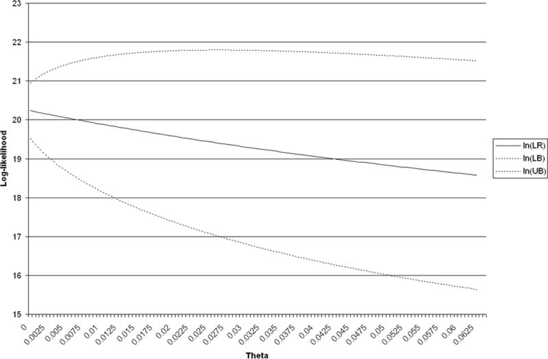
Log-likelihood ratio and 95% bounds, versus theta: most common alleles.

FIG. 2.

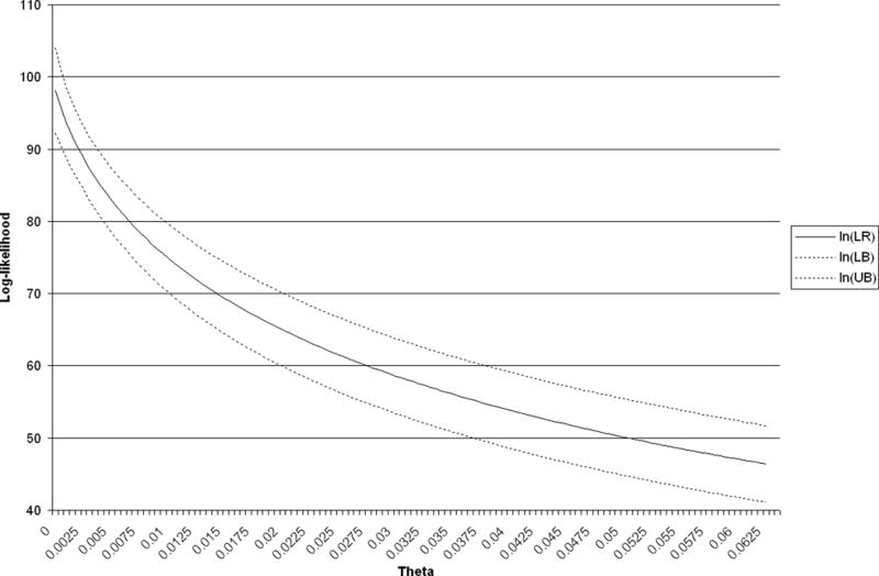
Log-likelihood ratio and 95% bounds, versus theta: least common alleles.

As with all classical confidence intervals, the sample size affects the width of the interval. Under the Dirichlet model, $\text{Var}({\stackrel{\sim }{p}}_{i,l})={\stackrel{\sim }{p}}_{i,l}(1-{\stackrel{\sim }{p}}_{i,l})(\theta +[(1-\theta )/2n_l])$. The (1 − θ)/2n goes to zero as the sample size goes to infinity. However, the θ cannot be eliminated by additional sampling within the population. This reflects the between-population variation.

Discussion

An explicit formula has been derived to allow the evaluation of confidence intervals for the likelihood ratios needed to interpret forensic DNA profiles. These intervals can be calculated with the computer program DNAMIX v.3, and they require details of the profile along with the frequencies of all alleles in the profile. The method applies to both single- and multiple-contributor profiles and allows for the incorporation of a population structure parameter θ. It is necessary to specify two alternative hypotheses for the contributors to the profile.

The method presented assumes profiles with several loci, such as the 13-locus CODIS set, in order for normal-distribution theory to be appropriate. The confidence intervals are symmetric on a logarithmic scale, so on the original likelihood ration scale, they provide intervals of the form $(\widehat{\text{LR}}\times C,\widehat{\text{LR}}÷C)$. Numerical work has shown that the factor $C=\text{exp}\left(z\frac{\alpha }{2}\sqrt{\text{Var}[\ln (\widehat{\text{LR}})]}\right)$ can be of the order of 100 or even 1000 for single-contributor stains, but it is probably <100 for multiple-contributor stains.

The population structure parameter θ describes the variation in allele frequencies over populations and allows the use of population-wide frequencies to apply to subpopulations or even frequencies from one population to apply to another population providing θ is sufficiently large. The underlying theory assumes that all populations have the same expected allele frequencies, but that the variance in frequencies among populations is proportional to θ. Numerical work has shown that, not only do likelihood ratios decrease as θ increases, but the confidence intervals increase in width with θ. In other words, the numerical value of the evidential strength of DNA profiles decreases as the variation among (sub)populations increases.

Appendix

Derivation of the Variance of the Confidence Interval

The most difficult part of calculating the confidence interval for a likelihood ratio is obtaining the variance of its logarithm. As we are assuming independent loci:

$$\begin{array}{l}\widehat{\text{LR}}={\displaystyle \prod _l{\widehat{\text{LR}}}_l}\\ \ln (\widehat{\text{LR}})={\displaystyle \sum _l\ln ({\widehat{\text{LR}}}_l)}\\ \text{Var}[\ln (\widehat{\text{LR}})]={\displaystyle \sum _l\text{Var}[\ln ({\widehat{\text{LR}}}_l)]}\end{array}$$

where LR is the likelihood ratio, and the loci are indexed by l. The Taylor expansion (δ-method) can be used to calculate an approximation of the variance for any function g of m variables:

$$\begin{array}{c}\text{Var}[g(x)]={\displaystyle \sum _{i=1}^m{\left(\frac{\partial g}{\partial x_i}\right)}^2}\text{Var}(x_i)\\ +{\displaystyle \sum _{i=1}^m{\displaystyle \sum _{j\ne i,j=1}^m\left(\frac{\partial g}{\partial x_i}\right)\left(\frac{\partial g}{\partial x_j}\right)}\text{Cov}(x_i,x_j)}\end{array}$$

The Taylor expansion can be applied to the logarithm of the likelihood ratio for the lth locus, with m variables being the m different allele frequencies (p_l,i) at the lth locus:

$$\begin{array}{c}\text{Var}[\ln ({\widehat{\text{LR}}}_l)]={\displaystyle \sum _{i=1}^m{\left(\frac{\partial \ln ({\widehat{\text{LR}}}_l)}{\partial {\stackrel{\sim }{p}}_{l,i}}\right)}^2}\text{Var}({\stackrel{\sim }{p}}_{l,i})\\ +{\displaystyle \sum _{i=1}^m{\displaystyle \sum _{j\ne i,\mathrm{j}=1}^m\left(\frac{\partial \ln ({\widehat{\text{LR}}}_l)}{\partial {\stackrel{\sim }{p}}_{l,i}}\right)\left(\frac{\partial \ln ({\widehat{\text{LR}}}_l)}{\partial {\stackrel{\sim }{p}}_{l,j}}\right)}\text{Cov}({\stackrel{\sim }{p}}_{l,i},{\stackrel{\sim }{p}}_{l,j})}\end{array}$$

The partial derivatives are

$$\begin{array}{l}\frac{\partial \ln ({\widehat{\text{LR}}}_l)}{\partial {\stackrel{\sim }{p}}_{l,i}}=\frac{\partial \{\ln [\text{Pr}(E_l|H_p)]-\ln [\text{Pr}(E_l|H_d)]\}}{\partial {\stackrel{\sim }{p}}_{l,i}}\\ =\frac{1}{\text{Pr}(E_l|H_p)}\frac{\partial \text{Pr}(E_l|H_p)}{\partial {\stackrel{\sim }{p}}_{l,i}}-\frac{1}{\text{Pr}(E_l|H_d)}\frac{\partial \text{Pr}(E_l|H_d)}{\partial {\stackrel{\sim }{p}}_{l,i}}\end{array}$$

We are using the same notation for the probabilities Pr (E_l|H) and their estimates that employ sample allele frequencies. For mixtures, Pr (E_l|H) is given by:

$$\begin{array}{c}\text{Pr}(E_l|H)={\displaystyle \sum _{r_1=0}^r{\displaystyle \sum _{r_2=0}^{r-r_1}\cdots }}{\displaystyle \sum _{r_{c-1}=0}^{r-r_1\dots -r_{c-2}}\frac{(2x)!2^{h_T+h_V}}{{\displaystyle {\prod }_{h=1}^c{u}_h!}}}\\ \times \frac{{\displaystyle {\prod }_{h=1}^c{\displaystyle {\prod }_{j=0}^{t_h+u_h+v_h-1}[(1-\theta ){\stackrel{\sim }{p}}_{l,h}+j\theta ]}}}{{\displaystyle {\prod }_{j=0}^{2x+2n_T+2n_V-1}[(1-\theta )+j\theta ]}}\end{array}$$

This equation is from equation 10 of Curran et al. (A1) and is fully explained there. The equation can be written in such a way that separates the terms containing the allele frequencies from those that do not. If K is the number of possible genotype combinations supported by the hypothesis and A_k the portion of the kth combination term that is invariant with respect to the allele frequencies:

$$\text{Pr}(E_l|H)={\displaystyle \sum _{k=1}^K{A}_k{\displaystyle \prod _{h=1}^c{\displaystyle \prod _{j=0}^{t+u_h+v_h-1}[(1-\theta )p_{l,j}+j\theta ]}}}$$

The required derivatives are

$$\begin{array}{c}\frac{\partial \text{Pr}(E_l|H)}{\partial {\stackrel{\sim }{p}}_{l,i}}=(1-\mathrm{\theta }){\displaystyle \sum _{k=1}^K{A}_k}\left({\displaystyle \prod _{h=1,h\ne i}^c{\displaystyle \prod _{j=0}^{t+u_h+v_h-1}[(1-\theta ){\stackrel{\sim }{p}}_{l,h}+j\theta ]}}\right)\\ \times \left({\displaystyle \sum _{q=0}^{t+u_h+v_h-1}{\displaystyle \prod _{j=0,j\ne q}^{t+u_h+v_h-1}[(1-\theta ){\stackrel{\sim }{p}}_{l,i}+j\theta ]}}\right)\end{array}$$

where ${\stackrel{\sim }{p}}_{l,i}$ is the sample frequency of the ith allele at the lth locus.

It is the expressions for the variances of allele frequencies that have proved problematic. Unlike the National Research Council 1996 report (A2), we consider that the variances are affected by the population structure parameter θ and under the same Dirichlet model that led to the result of Curran et al. (A1):

$$\begin{array}{l}\text{Var}({\stackrel{\sim }{p}}_{l,i})=p_{l,i}(1-p_{l,i})[(2n_l-1)\theta +1]/2n_l\\ \text{Cov}({\stackrel{\sim }{p}}_{l,i},{\stackrel{\sim }{p}}_{l,j})=-p_{l,i}{p}_{l,i}[(2n_l-1)\theta +1]/2n_l\end{array}$$ (1)

for samples of n_l individuals at locus l. Sample allele frequencies are substituted to provide estimates. We now explore the derivation of these expressions that are designed to accommodate variation in allele frequencies that is because of the evolutionary process as well as to the choice of sampled individuals.

A complete discussion makes a distinction between populations and subpopulations. Define indicator variables x_uvw for the wth allele drawn from the vth subpopulation of the uth population. These variables are equal to 1 if the allele is a particular type (i, say) and 0 otherwise. We suppose that only one population has been sampled but that the number of subpopulations is unknown. Alleles have relationships according to whether they are in the same subpopulation and in the same population. Dropping the locus and allele subscripts l and i, the expectations are (A3)

$$\begin{array}{l}\epsilon (x_{\mathit{uvw}})=\epsilon (x_{\mathit{uvw}}^2)=p\\ \epsilon (x_{\mathit{uvw}}{x}_{uv{w}^{\prime }})=p^2+p(1-p)\theta ,\text{different alleles}w\ne w^{\prime }\\ \epsilon (x_{\mathit{uvw}}{x}_{u{v}^{\prime }{w}^{\prime }})=p^2+p(1-p)\varphi ,\text{different subpopulations}v\ne v^{\prime }\\ \epsilon (x_{\mathit{uvw}}{x}_{u^{\prime }{v}^{\prime }{w}^{\prime }})=p^2,\text{different populations}u\ne u^{\prime }\end{array}$$

Suppose that n_v alleles have been taken from the vth of r subpopulation so that ${\displaystyle {\sum }_v{n}_v=n}$. Then, the sample frequency for population u is

$${\stackrel{\sim }{p}}_u=\frac{1}{n}{\displaystyle \sum _{v=1}^r{n}_v{\stackrel{\sim }{p}}_v=\frac{1}{n}{\displaystyle \sum _{v=1}^r{\displaystyle \sum _{w=1}^{n_{\nu }}{x}_{\mathit{uvw}}}}}$$

and

$$\begin{array}{l}\epsilon ({\stackrel{\sim }{p}}_u)=p\\ \epsilon ({\stackrel{\sim }{p}}_u^2)\\ =\frac{1}{n^2}\epsilon ({\displaystyle \sum _v{\displaystyle \sum _w{x}_{\mathit{uvw}}^2+{\displaystyle \sum _v{\displaystyle \sum _{w\ne w^{\prime }}{x}_{\mathit{uvw}}{x}_{\mathit{uv}{w}^{\prime }}}+{\displaystyle \sum _{v\ne v^{\prime }}{\displaystyle \sum _w{\displaystyle \sum _{w^{\prime }}{x}_{\mathit{uvw}}{x}_{u{v}^{\prime }{w}^{\prime }}}}}}}})\\ =\frac{1}{n^2}\{np+{\displaystyle \sum n_v(n_v-1)[p^2+p(-p)\theta ]}\\ +{\displaystyle \sum _{v\ne v^{\prime }}{n}_v{n}_{v^{\prime }}[p^2+p(1-p)\varphi ]}\}\\ \text{Var}({\stackrel{\sim }{p}}_u)=p(1-p)\left[\varphi +\frac{{\displaystyle {\sum }_v}{n}_v^2}{n^2}(\theta -\varphi )+\frac{1}{n}(1-\theta )\right]\end{array}$$

Bootstrapping would accommodate the variation among subpopulations (θ), but it would not address the variation among populations (ϕ).

Noting that ϕ ≤ θ (alleles are more related within than among subpopulations), a bound on the variance that does not depend on the number of subpopulations or how many alleles are sampled from each is found by setting ϕ = θ:

$$\text{Var}({\stackrel{\sim }{p}}_u)\le p(1-p)[\theta +\frac{1}{n}(1-\theta )]$$

which is the value we have used in this paper. It holds exactly if there are no subpopulations within the sampled population (r = 1, n₁ = n). The National Research Council (A2) used the binomial variances

$$\text{Var}({\stackrel{\sim }{p}}_u)=\frac{p(1-p)}{n}$$

which is appropriate if population structure is ignored (ϕ = θ = 0) or if every individual is in a different subpopulation (r = n; n_v = 1, v = 1, 2, …, r) and ϕ = 0.

We are concerned about the case when ϕ ≠ 0. One scenario would be when the single-sampled population is “Caucasians” and there is unknown substructure. The value of ϕ could be estimated by comparing Caucasians to other ethnic groups. Estimation of θ can be approximated by comparing Caucasians from different European countries. Note that, we expect θ to be greater than ϕ. If we take allele frequencies from different European countries and estimate “F_ST” by any standard method, we are actually estimating (θ − ϕ)/(1 − ϕ), whereas if we take frequencies from different ethnic groups, we are actually estimating ϕ (assuming that the ancestral human coancestry is zero) and the first estimate is smaller than the second.

When a sample is taken from a single population and there is no reason to suppose subpopulations, there is no distinction between θ and ϕ and r = 1. Protection against having the wrong population (wrong allele frequencies) is provided using $\text{Var}({\stackrel{\sim }{p}}_u)=p(1-p)[\theta +(1-\theta )/n]$. When a sample is taken from a single population but there is reason to suppose subpopulations, there is a distinction between θ and ϕ and r > 1. Protection against not recognizing the subpopulations (and using the wrong allele frequencies) is provided using Equation 1. It is conservative, in the sense of using an upper bound for this variance, to set ϕ = θ so that $\text{Var}({\stackrel{\sim }{p}}_u)=p(1-p)[\theta +(1-\theta )/n]$. This bound does not depend on how many alleles are sampled from each subpopulation.

Software

A computer program has been written to calculate the likelihood ratio, and its confidence interval. DNAMIX was originally written by Dr. John Storey and was updated to include the population structure calculations put forth by Curran et al. (A1). The current version, DNAMIX-3, has source code that is available and may be freely modified for research purposes. It is written in Java, so can be run on any operating system with Java installed. The program is available at http://www.biostat.washington.edu/~bsweir and is free to the public.

The formula used in DNAMIX-3 is slightly altered from that given by Curran et al. (A1): all allelic probabilities that are less than θ are replaced by the value of θ. This is to allow the calculation of LR for evidence profiles that contain alleles not seen in the database.

References

- 1.Torres Y, Flores I, Prieto V, Lopez-Soto M, Farfan MJ, Carracedo A, et al. DNA mixtures in forensic casework: a 4-year retrospective study. Forensic Sci Int. 2003;134(2–3):180–6. doi: 10.1016/s0379-0738(03)00161-0. [DOI] [PubMed] [Google Scholar]
- 2.Clayton TM, Whitaker JP, Sparkes R, Gill P. Analysis and interpretation of mixed forensic stains using DNA STR profiling. Forensic Sci Int. 1998;91(1):55–70. doi: 10.1016/s0379-0738(97)00175-8. [DOI] [PubMed] [Google Scholar]
- 3.Gill P, Brenner CH, Buckleton JS, Carracedo A, Krawczak M, Mayr WM, et al. DNA commission of the International Society of Forensic Genetics: recommendations on the interpretation of mixtures. Forensic Sci Int. 2006;160(2–3):90–101. doi: 10.1016/j.forsciint.2006.04.009. [DOI] [PubMed] [Google Scholar]
- 4.LaBerge GS, Shelton RJ, Danielson PB. Forensic utility of mitochondrial DNA analysis based on denaturing high-performance liquid chromatography. Croat Med J. 2003;44(3):281–8. [PubMed] [Google Scholar]
- 5.Cerri N, Ricci U, Sani I, Verzeletti A, De Ferrari F. Mixed stains from sexual assault cases: autosomal or Y-chromosome short tandem repeats? Croat Med J. 2003;44(3):289–92. [PubMed] [Google Scholar]
- 6.Weir BS, Triggs CM, Starling L, Stowell LI, Walsh KA, Buckleton J. Interpreting DNA mixtures. J Forensic Sci. 1997;42(2):213–22. [PubMed] [Google Scholar]
- 7.Curran JM, Triggs CM, Buckleton J, Weir BS. Interpreting DNA mixtures in structured populations. J Forensic Sci. 1999;44(5):987–95. [PubMed] [Google Scholar]
- 8.Triggs C, Harbison SA, Buckleton J. The calculation of DNA match probabilities in mixed race populations. Sci Justice. 2000;40(1):33–8. doi: 10.1016/S1355-0306(00)71931-9. [DOI] [PubMed] [Google Scholar]
- 9.Lauritzen SL, Mortera J. Bounding the number of contributors to mixed DNA stains. Forensic Sci Int. 2002;130(2–3):125–6. doi: 10.1016/s0379-0738(02)00351-1. [DOI] [PubMed] [Google Scholar]
- 10.Curran JM, Buckleton JS, Triggs CM, Weir BS. Assessing uncertainty in DNA evidence caused by sampling effects. Sci Justice. 2002;42:29–37. doi: 10.1016/S1355-0306(02)71794-2. [DOI] [PubMed] [Google Scholar]
- 11.Gill P, Foreman L, Buckleton JS, Triggs CM, Allen H. A comparison of adjustment methods to test the robustness of an STR DNA database comprised of 24 European populations. Forensic Sci Int. 2003;131(2–3):184–96. doi: 10.1016/s0379-0738(02)00423-1. [DOI] [PubMed] [Google Scholar]
- 12.Balding DJ, Nichols RA. DNA profile match probability calculation: how to allow for population stratification, relatedness, database selection and single bands. Forensic Sci Int. 1994;64(2–3):125–40. doi: 10.1016/0379-0738(94)90222-4. [DOI] [PubMed] [Google Scholar]
- 13.Balding DJ. Estimating products in forensic identification. J Am Stat Assoc. 1995;90:839–44. [Google Scholar]
- 14.Curran JM. An introduction to Bayesian credible intervals for sampling error in DNA profiles. Law, Probab Risk. 2005;4:115–26. [Google Scholar]
- 15.Hollander M, Wolfe D. Nonparametric statistical methods. New York, NY: Wiley-Interscience; 1999. [Google Scholar]
- 16.Weir BS. Genetic data analysis II. Sunderland, MA: Sinauer; 1996. [Google Scholar]
- 17.Evett IW, Weir BS. Interpreting DNA evidence: statistical genetics for forensic science. Sunderland, MA: Sinauer; 1998. [Google Scholar]
- 18.Budowle B, Moretti TR, Baumstark AL, Defenbaugh DA, Keys KM. Population data on the thirteen CODIS core short tandem repeat loci in African Americans, U.S. Caucasians, Hispanics, Bahamians, Jamaicans, and Trinidadians. J Forensic Sci. 1999;44(6):1277–86. [PubMed] [Google Scholar]