“Multi-wavelength single-molecule fluorescence analysis of transcription mechanisms”

Abstract

Multi-wavelength single molecule fluorescence microscopy is a valuable tool for clarifying transcription mechanisms, which involve multiple components and intermediates. Here we describe methods for the analysis and interpretation of such single molecule data. The methods described include those for image alignment, drift correction, spot discrimination, as well as robust methods for analyzing single-molecule binding and dissociation kinetics that account for non-specific binding and photobleaching. Finally, we give an example of the use of the resulting data to extract the kinetic mechanism of promoter binding by a bacterial RNA polymerase holoenzyme.

1. Benefits of single-molecule fluorescence in studying transcription mechanisms

Transcription is arguably the single most extensively regulated cellular process. Transcription regulation is biochemically complex for at least two important reasons. First, there are many intermediate steps between when an RNA polymerase molecule first binds to a promoter and when it finally transitions to a fully processive transcription elongation complex. Second, typical promoters are regulated by multiple transcription factors that interact with multiple binding sites on the DNA, on the polymerase, or both. As a result of these two phenomena, a given transcription template DNA molecule in a population can exist in one of tens or hundreds of different combinatorial states. This profusion of different chemical states makes analysis of mechanisms, particularly kinetic mechanisms, challenging to achieve by conventional bulk techniques that are restricted to studying the aggregate properties of a molecular ensemble.

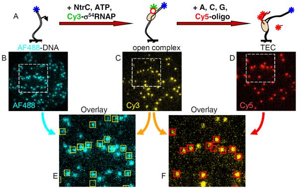
Over the last 20 years, the field has made a sustained and highly successful effort to circumvent the difficulties of ensemble analysis by using single-molecule light microscopy techniques to study transcription mechanisms (reviewed in [1–3]). Multi-wavelength single-molecule fluorescence co-localization approaches, which we term CoSMoS (co-localization single-molecule spectroscopy), have been used to explore both initiation mechanisms and the ways that transcription factors interact with DNA (e.g., refs. [4–8]). In a simple CoSMoS experiment (Fig. 1), a promoter-containing DNA tagged with a fluorescent dye is tethered to the surface of a microscope slide (e.g., by a biotin-streptavidin linkage). If the surface density of the DNA is low and the microscope is sufficiently sensitive, the individual dye molecules can be detected as discrete spots of fluorescence and the locations of the individual DNA molecules thus visualized (Fig. 1B). These tethered molecules then serve as “targets” with which “binder” molecules from solution can associate. For example, if one or more DNA-binding proteins (e.g., RNA polymerase; transcription factors) each labelled with a different color dye are added to the solution, the association and dissociation of these proteins with each individual DNA molecule can be monitored by observing a spot of binder fluorescence that co-localized to the position of a target molecule. By design, the dyes are attached to the molecules at locations sufficiently far apart that no fluorescence resonance energy transfer (FRET) can occur. The physical principle of the co-localization measurement is that only molecules that are linked at a fixed position on the surface produce a fluorescent spot; molecules free in solution move too rapidly and contribute only diffuse background fluorescence when observed on timescales > 1 ms. The approach can give a real time “movie” of the occupancy of an individual promoter DNA molecule and thereby allow determination of the kinetic mechanisms of initiation [4].

Figure 1. Example CoSMoS transcription experiment.

(A) A transcription initiation reaction was conducted in two discontinuous steps: glnAp2 promoter DNA molecules labeled with a fluorescent dye (AF488; blue star) were tethered to the slide surface. The reaction was initiated by introducing RNAP holoenzyme consisting of core RNAP (salmon) complexed with σ⁵⁴ (red circle) labeled with a second dye color (Cy3; green star) plus the activator NtrC and its cofactor ATP. These conditions lead to the formation of stable open complexes. Next, the nucleoside triphosphates (NTPs) ATP, CTP, and GTP are added along with an oligonucleotide probe labeled with a third color (Cy5, red star) that is used to detect the transcript RNA (red curve) by hybridization. (B–D) Fluorescence images (all of same surface region) in the three color channels acquired at the three reaction stages depicted in (A). (E–F) Dye colocalization reports complex formation. [Redrawn from ref. [4]]

In multi-wavelength single-molecule fluorescence experiments the most challenging aspects of the technique are often not the preparation of the molecules or making the microscope observations, but in analyzing the resulting data. Data analysis has two primary challenges. First, one is studying inherently stochastic processes (thermally driven reactions of single molecules), so that analysis is inherently statistical. Second, the number of photons that can be emitted by a single fluorophore is limited by photobleaching, so images often have low signal-to-noise ratios, making discrimination of real signals from noise a challenge. In this article, we summarize the fundamental steps in the process of data analysis. These include mapping, drift correction, spot discrimination, kinetic analysis (measurement of association and dissociation rate constants), and mechanistic interpretation. Each of these topics is discussed in a separate section below. The descriptions here are not comprehensive, they simply describe some of the particular approaches that we have used in our experiments. While the discussion focuses on studying transcription, many of the approaches that we describe here can be used to study the mechanisms of other complex biochemical processes [9–12].

2. Alignment of images from multiple wavelength channels

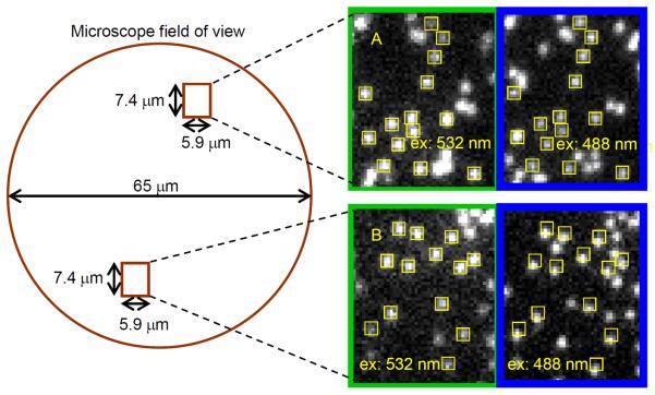
In multi-wavelength single-molecule fluorescence co-localization experiments, images of the microscope field of view are recorded from each of the wavelength channels (i.e., excitation/emission wavelength pairs) corresponding to the different fluorophores being used. An essential step in data analysis is to define the physical locations in images from one channel that correspond to the same locations recorded in the other channels. We call the process of establishing these relationships “mapping”. Different wavelength images may be recorded simultaneously, or in rapid alternation. Simultaneous acquisition often uses dual-view optics, which spatially offset images on the camera sensor based on the emission wavelengths (e.g., simultaneously producing an image of Cy5 emissions >635 nm and a second image of Cy3 emissions <635 nm). Even when dual-view optics are not used and images for different wavelength channels are alternately collected on the same area of the camera sensor (time multiplexing), mapping may still be necessary to correct for spatial distortions in the images (e.g., from chromatic aberration) (Fig. 2).

Figure 2. Chromatic distortion in time-multiplexed imaging.

Surface-tethered oligonucleotide molecules each labeled with both Cy3 and Alexa Fluor 488 (AF488) were imaged in rapid succession with excitation wavelengths 532 nm (Cy3) and 488 nm (AF488). Yellow squares mark the same pixel locations in the two images. Magnified views show that images from one part of the microscope field of view are well aligned (A), whereas distortions misalign another part of the same image (B).

For each dye labeled DNA molecule attached to the slide surface, precise (x, y) coordinates are determined by independently fitting the pixels in a square region around each spot image to a two-dimensional Gaussian

$$I(X,Y)=I_o\text{exp}(-[{(X-x)}^2+{(Y-y)}^2]∕(2{\sigma }^2\left)\right)+H,$$ (1)

where I_o, x, y, σ, and H are fit parameters.

To determine the position in channel 2 (x₂, y₂) that is equivalent to the position of a spot in channel 1, (x₁, y₁), we apply the transformation

$$\begin{array}{cc}\hfill & x_2=A{x}_1+B{y}_1+C\hfill \\ \hfill & y_2=D{x}_1+E{y}_1+F,\hfill \end{array}$$ (2)

where A-F are fit parameters. Because the values for these parameters vary systematically across the microscope field of view, we determine their values separately for each spot coordinate (x₁, y₁) by local fitting [13] of Eq. 2 to pairs of corresponding points determined from calibration images. In particular, we use the 15 calibration pairs nearest to (x₁, y₁) (which are typically within a 4.5 to 6.5 μm distance) to determine the best fit parameter values that apply to (x₁, y₁).

Typically, we collect one set of calibration images on each day of experiments. A convenient calibration sample contains a surface-anchored DNA oligonucleotide, each molecule of which is hybridized with a set of shorter oligonucleotides [14] that are labeled with the same dyes used in the experimental samples. Use of the same dyes minimizes chromatic aberration differences between calibration and experimental samples. The oligonucleotide design allows ready preparation of samples with the precise combination of dyes needed, and the dye spacing can be made large enough to minimize FRET (fluorescence resonance energy transfer) between dyes. Accurate mapping requires a high density of calibration points to adequately compensate for geometric aberration and other factors [15–17]; we typically prepare samples with ~300 randomly distributed molecules per 65 μm diameter microscope field and collect images from ~9 fields of view.

The data derived from the calibration sample consists of a calibration list of N_p pairs of corresponding spot coordinates from the two channels:

$$(x_1^i,y_1^i)\leftrightarrow (x_2^i,y_2^i)i=1to{N}_p,$$ (3)

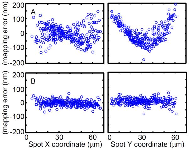
where the subscripts 1 and 2 refer to the two channels. Since the calibration images have large numbers of spots, we employ an automated spot-detection algorithm [18,19] that enables us to batch process hundreds of spots. The algorithm is tuned by specifying spot amplitude and diameter thresholds. However, not all detected spots in the calibration sample are included in the calibration list. Incomplete labeling of the oligonucleotides will cause spots of one color to not have matching partners of the other color. This can lead to incorrect spot pair assignment for mapping. To minimize these complications we follow a calibration list construction procedure (Protocol 1). The result is a self-consistent list that usually contains from 400 to 800 coordinate pairs (Eq. 3) and produces mapping results that are limited only by the accuracy of the spot position measurements (Fig. 3).

Figure 3. Mapping error.

Graphs indicate the differences between actual position of a spot and the mapped position of its partner for 273 spots in a test image. For this experiment, the calibration data and test image were collected from different fields of view from a sample of surface-tethered DNA oligonucleotides labeled with Cy3 and Cy5 under illumination with a 532 nm laser. This oligonucleotide was designed so that Cy5 was excited through FRET, so that all Cy5 spots have a Cy3 partner. Coordinates of Cy5 spots are mapped into the Cy3 field and compared with the known locations of their Cy3 spot partners. (A) Global mapping using all calibration points for each spot causes large errors that vary systematically with spot position across the microscope field. (B) Local fitting using only the 15 closest calibration points (see text) eliminates systematic variation and produces r.m.s. errors (19 and 21 nm in x and y, respectively) close to the variation expected from the uncertainty in the position measurements alone (19 nm measured over all pairwise combinations of N = 130 spot position differences measured over 100 s [28]).

In experiments that use three colors we typically produce three different calibration lists to perform mappings between all three possible pairwise combinations of images. In addition to its use in identifying corresponding spots in images from two different wavelength channels, the same mapping protocol can also be used to connect images in the same wavelength channel acquired before and after an interruption in data acquisition, such as those which may be required to introduce new reagents into the sample.

3. Drift correction

Mechanical instability in the microscope optics can cause apparent slow movement of the sample in the microscope image. Movement can also be caused by experimental manipulations (e.g., introducing a new solution into the sample chamber). It is often necessary to correct for these drift movements so that individual target molecules can be followed over time, particularly when observation of the same field of view extends over minutes or hours. In our microscopes, movements are typically small (a few pixels over a period of an hour), so we find it most convenient to compensate for drift during data analysis, rather than by moving the microscope stage during image acquisition.

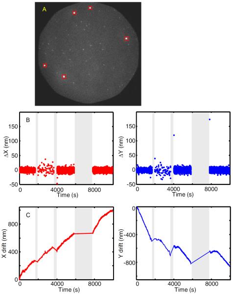
The simplest way to collect the information needed for drift correction is to include on the sample chamber surface bright fiducial markers that show a fluorescence signal that remains visible throughout image acquisition. For example, polystyrene beads derivatized with multiple fluorescent dyes are commercially available and can be included at surface density sufficient to give 1–5 beads in each field of view. Bead images are typically bright enough that they are readily distinguishable from the weaker fluorescence from molecules labeled with single dyes (Fig. 4A). Gaussian fitting of a bead fluorescent spot in successive frames produces a record of bead movement, which is summarized in a table listing the Δx and Δy movement between each frame interval during an recording (Fig. 4B,C). When photostable beads are not present, it is still possible to construct a drift table using the single-dye fluorescence spots of the molecules being studied. Single dye spots typically do not last through the entire duration of an experiment, but drift records data from multiple spots can be averaged (when overlapping in time) and stitched together to construct the necessary (Δx, Δy) table.

Figure 4. Drift correction.

(A) Spots from bright fluorescent beads (40 nm diameter TransFluoSpheres, Life Technologies, T10711) marked by squares are readily distinguishable from fluorescence of single dye molecules on a DNA oligonucleotide used to detect a nascent transcript by hybridization (unmarked spots). (B) Plots of the drift table data Δx and Δy against time. Images were recorded using four 0.24 s duration frames every 100 s between time 1950 – 3630 s and recorded continuously using frames of duration 1 s elsewhere. Interruptions in the drift table (gray) are intervals when image acquisition was temporarily suspended. (C) Integrals of the drift table which display the net drift in x and y.

To correct for drift in dual-field imaging, we form separate drift tables for each field. This may be done either by independently finding the centers of fiducial markers in the two fields or by constructing a drift table for one field and then mapping the resulting (x, y) track (Figure 4B, bottom) into the second field.

The drift table is used to identify the positions corresponding to the location of a target molecule in two frames recorded at different times. Specifically, the coordinate displacements that occur for a molecule between frame m and frame n (for n > m) are calculated by summing the Δx or Δy values in the drift table for the frames spanning m to n.

4. Spot discrimination

Having analyzed image mapping and drift, the next step in analysis of single-molecule co-localization data is to compile information about when a binder molecule fluorescence spot is observed at the surface position of a target molecule. For example, one may wish to tabulate when, for each AF488-labeled DNA molecule, a co-localized spot of Cy3-RNA polymerase (or a transcription factor) fluorescence is observed (Fig. 1).

First, we identify a set of target molecules and their corresponding locations in the binder images. We usually identify surface-tethered DNA molecules in an image collected before other reaction components are added. Analogously to the procedures used for mapping, a list of target positions is created by automated spot-detection and spot pairs that are too closely spaced are removed. During the analysis, the positions corresponding to target molecule locations in each frame of the binder molecule channel recording are then identified by applying the mapping and drift correction data.

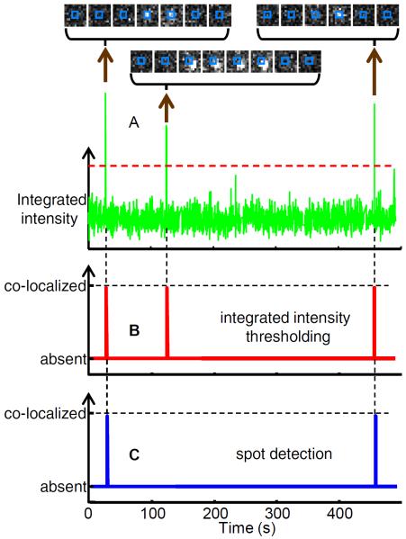
The initial goal is to translate the images into binary time records that summarize when binder is co-localized with each target (Fig. 5). One method [4,9,11] relies on integrating the binder fluorescence intensity over small regions of the image (e.g., squares 0.4 μm on a side) centered on the mapped, drift-corrected location of the target molecule. Co-localized appearance and disappearance of the binder spot are accompanied by abrupt increase and decrease of the integrated fluorescence. The time interval during which the binder is present is defined by applying distinct high and low integrated intensity thresholds to identify the interval beginning and end. False positives are common with this method due to binder molecule association with nearby target molecules (Fig. 5A,B) and diffusion of brightly fluorescent particulates above the surface. It is usually necessary to visually inspect the images that accompany each identified landing interval to remove those false positives and improve detection accuracy. However, visual inspection introduces an undesirable subjective aspect to the data analysis, and it is impractical on large datasets.

Figure 5. Spot discrimination.

(A) Integrated fluorescence intensity and selected images of binder molecules (Cy3-GreB) co-localizing with an individual target molecule (a transcription elongation complex). Intensity is integrated over a 0.4 × 0.4 μm square at 4 frames s⁻¹; images are 1.3 × 1.3 μm and the integration area is marked (blue). (B) Co-localization intervals scored from integrated intensity (see text) using the intensity thresholds shown as dashed lines in (A). (C) Co-localization intervals scored by spot detection (see text). Note that this algorithm scores only the first and third peaks in (A), rejecting the middle event because the binder spot was not well-centered on the target location.

A superior method (Fig. 5C) [5] makes use of aspects of the binder spot image data (e.g., size, shape, intensity profile, and precise distance to target) that are disregarded when only the integrated intensity is used. We first apply to all frames in the image sequence the same spot-detection algorithm used in the mapping procedure. This spot detection is applied twice to each image, using a high spot amplitude threshold to avoid false positives and a low spot amplitude threshold to avoid false negatives (Fig. 6). The start of a co-localization interval is scored when a binder spot center is detected within a set distance (e.g., 180 nm) of the target while using the high intensity threshold. The interval is scored as ending during the first subsequent frame in which a binder spot is not detected within 270 nm of the target location using the low intensity threshold. The less stringent criteria used to score interval ends helps to minimize instances in which a single binding event might be incorrectly scored as multiple bindings of shorter duration. Intervals that are between binder co-localization intervals are designated binder absent intervals. For further analysis, intervals in each binary trace are summarized in a data structure (the `intervals table') that records the location, time, duration, and type of each interval (Fig. 7). Intervals that begin or end a data record are marked as such because these require special treatment in some data analyses as noted below.

Figure 6. Effect of the amplitude threshold setting in the spot detection algorithm.

(A) Circular 65 μM diameter binder channel image. There are two bright spots due to 40 nM fluorescent bead fiducial markers and ~70 dimmer spots arising from Cy3B-GreB binder molecules bound to transcription elongation complex targets. (B, C) Magnified view of the 13.2 × 13.2 μm region enclosed by the dotted yellow line in (A). The spot detection algorithm detects 6 spots (red squares in (B)) at the high spot amplitude threshold equal to 25 and 60 spots (C) at the low threshold equal to 9. Images in (A–C) are reproduced at high contrast to emphasize image noise. (D) The number of detected spots (blue) for the field of view shown in (A) varies with the amplitude threshold setting. At low amplitude settings (i.e., <20) the algorithm identifies image noise features as spots, resulting in an excessive number of detected spots. The data are fit with a bi-exponential function (red) consisting of one term approximating the number of false positive spots due to image noise (green) and a second term approximating the number of true binder spots (black). The fits are used to calculate a threshold (dashed line) for which there is an estimated 50% probability of having no noise-induced spots detected within 1 pixel of a single DNA location during the 4000 frame duration experiment.

Figure 7. Coding binding interval data.

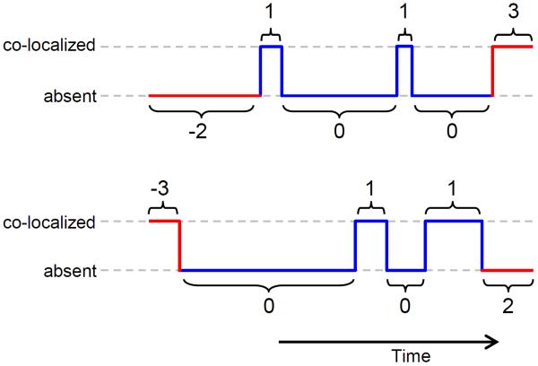
Plots illustrate two schematic data records consisting of alternating binder co-localization (top brackets) and binder absent (bottom brackets) intervals. Co-localization and absent intervals are coded as −3 and −2 respectively when they are the first (or only) interval in a record, 3 and 2 when they are the last interval in a record and 1 and 0 elsewhere.

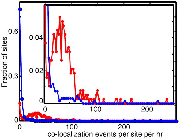
Using the above spot detection based method avoids the necessity of visually inspecting all scored binding events to remove false positives. Nevertheless, we occasionally find that a small number of target molecules account for a disproportionately large number of binder co-localization intervals. This can occur because of binding to an unlabeled target molecule adjacent to the labeled target being measured, resulting in a binder spot that is borderline with respect to either the intensity or proximity threshold. Statistical methods can be used to exclude these anomalous target locations from subsequent analyses (Fig. 8) when the anomalies arise from such experimental artefacts and not from actual heterogeneity in target molecule behaviors.

Figure 8. Identification of outlier target molecules.

Example of a histogram recording the frequency of binder co-localization intervals recorded at each target location during an experiment (red; in this case, GreB binding to transcription elongation complexes over 25 min.) and to randomly selected control locations that lack visible target molecules and therefore reflect non-specific surface binding (blue). Inset: Magnified view. The peak in the red curve centered at ~33 co-localization events per site per hr represents the behavior of typical target molecules; the tail at > 120 represents rare (9% of total) outlier target molecules that were excluded from subsequent analysis.

5. Measuring association rate constants

The ability to observe individual protein molecules associating with DNA, for example, RNA polymerase molecules binding to a promoter, allows direct measurement of association kinetics uncomplicated by the participation of isomerization steps that follow binding [4,5]. To measure the association rate at a particular solution concentration of binder (e.g., RNA polymerase), we ordinarily use the absent intervals that precede the first observed binding interval (i.e., the intervals coded −2 in Fig. 7). The statistics of those intervals will in principle match those of the larger data set of intervals separating successive bindings (i.e., those coded 0 in Fig. 7). However, in practice the use of only the intervals that precede the first event greatly reduces artefacts caused by the effects of binder photobleaching (intervals in which target molecules are occupied by photobleached binder will be erroneously scored as absent intervals) and negative dropouts (in which a single binding event is scored as multiple co-localization intervals separated by spurious short absent intervals).

For most experiments there is some binder co-localization that occurs even at randomly chosen sites that do not contain a visible target molecule. This may result from transient non-specific interactions of the binder protein with the chamber surface (or possibly from specific binding to rare non-fluorescent target molecules). This “nonspecific” binding contributes to the association rate recorded at all locations and we must account for it when measuring the specific association rate to target. To measure the non-specific rate, we pick N_c control locations that do not overlap target sites (Fig. 9). For these sites we compile a list of initial absent intervals {τ_cj} that correspond to the time elapsed prior to the first binder co-localization at the control location (i.e., those coded −2 in Fig. 7). We also separately count the number n_c of control locations at which no binding occurs throughout the entire observation interval T_max. To derive the nonspecific binding rate constant k_ns we fit these data using a maximum likelihood algorithm [20,21] in which we vary k_ns to maximize the likelihood function associated with all N_c observations:

$$G_{ns}\left(k_{ns}\right)=\text{exp}(-n_c{k}_{ns}{T}_{\text{max}})\prod _{j=1}^{N_c-n_c}{k}_{ns}\text{exp}(-k_{ns}{\tau }_{cj}).$$ (4)

In Eq. 4, each factor of k_nsexp(-k_ns τ_cj) is proportional to the probability of observing a time-to-binding interval of length τ_cj and each of the n_c factors of exp(-k_nsT_max) is the probability of not observing any binding during the entire observation interval T_max (or equivalently, the probability of observing a binding at some time during the interval from time T_max to infinity). (To accommodate the limited precision of digital representation of real numbers, we maximize the sum of the logarithms of the individual factors instead of their product.)

Figure 9. Tabulating control locations devoid of target spots.

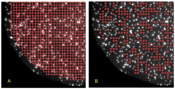
Two identical images (32 × 32 μm) of a portion of a microscope field of view showing target fluorescent DNA spots. (A) A close-packed grid of 9 × 9 pixel (1.2 × 1.2 μm) squares (red) was constructed to cover the field of view. (B) The automated spot-detection algorithm was used to remove any square from (A) whose center is closer than 8 pixels (1.06 μm) to any detected spot. The remaining squares were reduced to a 4 × 4 pixel size.

Having determined the rate constant for non-specific binding to the surface, we next analyze the specific binding to target molecule locations. For the N target sites we tabulate (1) the number n of sites at which no binder co-localization was observed throughout the entire observation interval T_max, (2) the number n_z of sites for which co-localized binder was already detected at the beginning of the recording (i.e., code −3 in Fig. 7), and (3) a list of initial absent intervals {τ_j} that correspond to the time elapsed prior to the first binder co-localization at the target location (i.e., those coded −2 in Fig. 7).

These data are fit (Fig. 10A) to a model that assumes there are two subpopulations of target molecules: an active fraction A_f ≤ 1 that exhibits binder co-localization at a rate (k_a + k_ns), where k_a is the specific apparent first-order association rate constant, and an inactive fraction (1 − A_f) that shows only nonspecific binding at the same k_ns rate found at the control locations. The active faction includes the n_z sites at which co-localized binder was already detected at the beginning of the recording. In this model, the probability for each τ_j observation given chosen values k_a and A_f is proportional to

$$P_o({\tau }_j\mid k_a,A_f)=(A_f-\frac{n_z}{N})(k_a+k_{ns})\text{exp}[-(k_a+k_{ns}\left){\tau }_j\right]+(1-A_f)k_{ns}\text{exp}[-k_{ns}{\tau }_j],$$ (5)

and the probability of each of the n observations of targets with no binder co-localization is

$$P_{no}(T_{\text{max}},k_a,A_f)=(A_f-\frac{n_z}{N})\text{exp}[-(k_a+k_{ns}\left)T_{\text{max}}\right]+(1-A_f)\text{exp}[-k_{ns}{T}_{\text{max}}].$$ (6)

Therefore, to derive k_a and A_f we vary those parameters to maximize the likelihood function

$$G(k_a,A_f)={\left(P_{no}\right(T_{\text{max}},k_a,A_f\left)\right)}^n\prod _{j=1}^{N-n-n_z}{P}_o({\tau }_j\mid k_a,A_f).$$ (7)

Figure 10. Association kinetics of GreB with transcription elongation complexes.

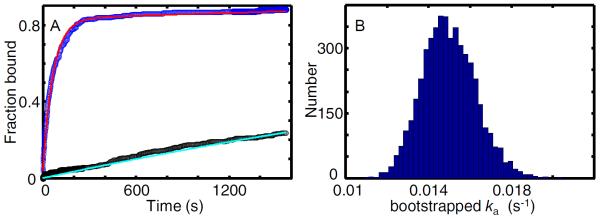
(A) Cumulative fractions of surface-tethered elongation complex targets (blue; N = 287) and control sites (black; N_c = 382) at which GreB (0.5 nM) co-localized at least once prior to the indicated time. Fitting (see text) was used to calculate model curves based on Eq. 5 (red; k_a = (1.49 ± 0.13) × 10⁻² s⁻¹ and A_f = 0.83 ± 0.02) and an exponential probability density function (cyan; k_ns = (1.75 ± 0.19) × 10⁻⁴ s⁻¹). (B) Estimated uncertainty in k_a. The plot is a histogram of k_a values derived from fitting 5,000 bootstrap samples of the data in (A). The standard deviation of these values (0.13 × 10⁻² s⁻¹) is the estimated standard error of k_a reported in (A).

To determine the standard error in the fit parameters k_a, A_f, and k_ns, we use a bootstrap calculation [22]. The N_c observations made at control sites are listed in a table that includes both the n_c observations of no co-localization plus the N_c−n_c observations of {τ_cjinitial absent intervals. We generate a large number (typically 5,000) simulated data sets. To generate each such set, we randomly sample with replacement N_c values from the observations table. Each bootstrapped data set is then fit by maximizing Eq. 4 to yield an estimated k_ns. We then generate bootstrapped data sets from the list of N experimental observations made at target sites. In that instance we randomly sample with replacement from a table that includes n observations of no binder co-localization, n_z observations of binder co-localization at time zero and N–n–n_z observations of the {τ_j} initial absent intervals. We also randomly sample a k_ns value from the set calculated in the prior bootstrap. These sampled data are then together fit by maximizing Eq. (7) to determine values for k_a and A_f. Repeated bootstrapping yields simulated distributions for k_ns, A_f and k_a (e.g., Fig. 10B); the standard deviation of each distribution yields the estimated standard error of the corresponding parameter.

For bacterial RNA polymerase molecules binding to promoter DNA targets (e.g., ref. [5]) and transcription factors binding to transcription complexes (e.g., Fig. 10), this approach typically yields fits in close agreement to the experimental data. The slow increase in the target curve after 200 s is not mechanistically significant; the model explains this as slow non-specific binding to the surface at the fraction of target sites that are inactive to specific binding.

6. Measuring dissociation rate constants

The lifetime of co-localization intervals can provide information about the dissociation rate of the binder-target complex. Furthermore, the distribution of co-localization intervals can reveal the existence of multiple types of these complexes, their mechanism of interconversion and their relative kinetic stabilities. Typically, co-localization interval distributions are the sum of multiple exponential terms reflecting the presence of multiple types of binder-target complexes. In general, more than one type of complex contributes to each term in the distribution [23,24].

To measure the lifetimes of binder-target complexes, we first tabulate the durations of co-localization intervals (coded −3 and 1 in Fig. 7) at N target and N_c non-target sites. To get an initial idea of the distribution of target-specific co-localization intervals, we subtract the non-target from the target data:

$$n_m^s=n_m-n_m^c\left(\frac{T}{T_c}\right).$$ (8)

where n_m and $n_m^c$ are the measured numbers of co-localization intervals with durations lasting m frames detected at target and non-target sites, respectively; and T and T_c are the sum of the durations of all absent intervals (coded −2, 0 and 2 in Fig. 7) observed at target and non-target sites, respectively. The $n_m^s$ values are then the estimates of target-specific co-localizations with duration lasting m frames, which can be summarized in a histogram to visualize the shape of the distribution of co-localization durations.

Once the shape of the distribution is known, we proceed to a more quantitative, model-dependent analysis. Typically, co-localization intervals can be recorded only when their duration exceeds a minimum t_min that is set by experimental conditions [20]. We model the {τ_cj}interval durations that occur at non-target sites as arising, for example, from a bi-exponential probability density distribution

$$P_2(t\mid r_{1c},r_{2c},a_c)=\frac{a_c{r}_{1c}\text{exp}[-r_{1c}t]+(1-a_c)r_{2c}\text{exp}[-r_{2c}t]}{a_c\text{exp}[-r_{1c}{t}_{\text{min}}]+(1-a_c)\text{exp}[-r_{2c}{t}_{\text{min}}]},$$ (9)

where a_c is the relative amplitude and r_1c and r_2c are two characteristic departure rates. As written, P₂ is normalized so that it integrates to 1 over durations t greater than t_min. We maximize the likelihood function

$$G_d^c(r_{1c},r_{2c},a_c)=\prod _{j=1}^{L_c}{P}_2({\tau }_{cj}\mid r_{1c},r_{2c},a_c),$$ (10)

where L_c is the total number of observed co-localization intervals (typically a few hundred to one thousand) at the non-target sites, thus obtaining values for a_c, r_1c, and r_2c.

Correcting the co-localization interval distributions measured at target locations for the nonspecific binding contribution requires that we again account for the relative frequencies of co-localizations at target vs. non-target sites. The non-target site frequency is A_c = L_c / T_c and the target site frequency is similarly A = L / T where L is the total number of observed co-localization intervals. We then model the frequency distribution of interval durations at target sites as

$$F(t\mid r_1,r_2,a,r_{1c},r_{2c},a_c)=(A-A_c)P_2(t\mid r_1,r_2,a)+A_c{P}_2(t\mid r_{1c},r_{2c},a_c)$$ (11)

so that F(t|r₁,r₂,a,r_1c,r_2c,a_c)dt is the predicted rate of co-localization intervals with durations between t and t+dt that occur at one target site. Eq. 10 separates the binding frequency contributions into a first term for co-localizations that are target-specific and a second term for those that are non-specific. For the L observed co-localization durations at target sites {τ_j} we maximize the likelihood function

$$G_d(r_1,r_2,a)=\prod _{j=1}^{L}F({\tau }_j\mid r_1,r_2,a,r_{1c},r_{2c},a_c),$$ (12)

by varying the values of r₁, r₂, a (using the fixed values for r_1c,r_2c, and a_c determined earlier).

Once the data have been fit, it is useful to visually compare plots of the distribution of data and the distribution predicted by the fit parameters and model. For example, the plot in Fig. 11A compares data and a fit for co-localization of σ⁵⁴RNA polymerase on a promoter DNA target. The data plot is a cumulative frequency distribution, in which each point represents the average frequency at which binder co-localization intervals (coded −3 and 1 in Fig. 7) longer than the specified co-localization duration occur at a target location. The fit is a plot of the function

$$R(t,r_1,r_2,a,r_{1c},r_{2c},a_c)=(A-A_c)S_2(t,r_1,r_2,a)+A_c{S}_2(t,r_{1c},r_{2c},a_c),$$ (13)

where

$$S_2(t,r_1,r_2,a)=\frac{a\exp [-r_{1}t]+(1-a)\exp [-r_{2}t]}{a\exp [-r_1{t}_{\min }]+(1-a)\exp [-r_2{t}_{\min }]}.$$ (14)

Eq. 13 consists of contributions arising from the DNA-specific (first term) and the nonspecific (second term) co-localization intervals.

Figure 11. Plotting co-localization interval distributions and their fits to models.

All three panels show plots of the same example data set (taken from ref. [5]) of 0.1 nM σ⁵⁴RNA polymerase binding to 3,591 bp target DNA molecules containing a σ⁵⁴ promoter (blue, N = 122 DNA, L = 1000 co-localizations) and to non-target control sites (black, N_C = 157, L_C = 129). Data were fit using biexponential distributions for both the target sites (red; r₁ = 0.34 s⁻¹, r₂ = 1.6 × 10⁻² s⁻¹, and a = 0.85; Eqs. 11 and 12) and the non-target sites (cyan; r_1c = 0.75 s⁻¹, r_2c = 2.4 × 10⁻³ s⁻¹, and a_c = 0.96; Eqs. 9 and 10). (A) Cumulative frequency distributions of co-localization intervals at target and non-target sites. Inset: semilog plot of the same data on an expanded timescale. (Redrawn from ref. [5].) (B) Same data and fit as in (A), with the bootstrap estimate of the 95% confidence limits (dashed) of the data. (C) The data and fit from (A) visualized as a probability density function (± s.e.).

In judging the agreement between data and fit curve, it is important to remember that in this type of plot the statistical deviations of each successive data point are not independent. Indeed, each point in the cumulative frequency distribution includes the random experimental errors of all points to its right. This is why we do not directly fit the cumulative curve using a conventional fitting procedure that assumes independent errors; instead we use maximum likelihood methods to directly fit the underlying observations as described earlier. To visualize the statistical uncertainty in the cumulative distribution curve, we construct a family of curves from bootstrap samples of the experimental data and plot the envelope for the 95% confidence interval of the family (Fig. 11B).

An alternative visualization of the data is to plot a binned probability density histogram [20]. Colocalization events are sorted into bins that record the number of co-localizations n_i with durations between the limits of the ith bin. The probability density in bin i is then

$$p_i=n_i∕\left(L{w}_i\right),$$ (15)

where L is the total observed number of co-localized landings at all target sites and w_i is the width of the i^th bin (Fig. 11C). The standard error in each p_i is the binomial uncertainty (n_i [1−(n_i/L) ])^1/2 /( Lw_i ). These errors are statistically independent for each bin. In the probability density function representation, the fit curve is plotted as the model probability density function F(t, r₁, r₂, a, r_1c, r_2c, a_c)/A (see Eq. 11).

The apparent departure rates as determined above will in general have contributions from both the rate of dissociation of binder from target and from photobleaching of the dye label on the binder. Photobleaching has the most pronounced effects on the slower terms of multi-exponential lifetime distributions. To measure dissociation kinetics independent of photobleaching, we repeat experiments using different amounts of exposure to the excitation laser and extrapolate the results to zero exposure. A convenient way to vary exposure is to keep the laser power constant but to vary the fraction of time I during which the sample is exposed to the laser (for example, I = 1 for continuous exposure, whereas I = 0.1 for a time lapse acquisition in which the laser is alternately on for 1 s and off for 9 s) [25]. The rates measured at different exposure fractions r(I) can then be fit to

$$r\left(I\right)=r_o+Ib,$$ (16)

yielding values for the fit parameters r_o, the photobleaching-independent dissociation rate, and b, the photobleaching rate at continuous exposure.

7. Deducing reaction mechanisms from single-molecule kinetics

The analysis outlined above enables us to summarize the kinetics of co-localization intervals and binder-target association in terms of probability distributions. Those distributions may contain multiple exponential terms, and the rates associated with those terms are mathematically related to (but not generally the identical to) rate constants in the kinetic mechanism of the reaction. Well established methods exist to relate single-molecule probability distributions to kinetic mechanisms (for example in refs. [23,24]). Here we illustrate the process using the example of a bi-molecular association followed by a conformational isomerization, the mechanism of closed promoter complex formation by σ⁵⁴RNA polymerase enzyme (E) at the glnAP2 promoter (D) in the absence of activator [4]. In that instance two distinct closed complex species form, and the appropriate reaction scheme is

$$\mathrm{E}+\mathrm{D}\underset{k_{-1}}{\overset{k_a}{\rightleftarrows }}{\left(\mathrm{E}•\mathrm{D}\right)}_1\underset{k_{-2}}{\overset{k_2}{\rightleftarrows }}{\left(\mathrm{E}•\mathrm{D}\right)}_2,$$ (17)

where (E•D)₁ is a short-lived closed complex, (E•D)₂ is a long-lived closed complex, and the pseudo first-order rate constant k_a = k₁[E], where k₁ is the second-order binding rate constant and [E] is the polymerase concentration.

The Eq. 17 mechanism predicts a single exponential target-specific association distribution (Eq. 5) and a bi-exponential co-localization interval distribution (Eqs. 9 and 11). In this instance the association rate measured in our single molecule binding experiment (the rate k_a in Eq. 5) is identical to the rate constant k_a appearing in the reaction scheme (Eq. 17). In contrast, the values of k₋₁, k₋₂, and k₋₂ in Eq. 17 do not directly correspond to any measured rate. However, the values of these rate constants can be derived from the parameters of the co-localization interval distribution (Eq. 11) as follows:

Each RNA polymerase that binds a promoter first occupies the (E•D)₁ state at time t = 0. The fraction of binding events in which the polymerase still remains bound (i.e., in either (E•D)₁ or (E•D)₂) at time t > 0 is:

$$-\frac{(k_2+k_{-2}-r_1)}{r_1-r_2}{e}^{-r_{1}t}+\frac{(k_2+k_{-2}-r_2)}{r_1-r_2}{e}^{-r_{2}t},$$ (18)

where r₁ and r₂ are the measured rates that appear in the Eq. 11 co-localization interval distribution. The relative weights of the two components in Eq. 11 are then given by the ratio of coefficients in Eq. 18, so that

$$\frac{\mathrm{a}}{(1-\mathrm{a})}=-\frac{(k_2+k_{-2}-r_1)}{(k_2+k_{-2}-r_2)},$$ (19)

and the measured relaxation rates r₁ and r₂ are given by the two roots

$$r_{1,2}=\frac{(k_{-1}+k_2+k_{-2})\pm \sqrt{{(k_{-1}+k_2+k_{-2})}^2-4k_{-1}{k}_{-2}}}{2}.$$ (20)

Given values of r₁, r₂, and a, Eqs. 19 and 20 can be numerically solved to yield k₋₁, k₋₂ and k₂; for example, r₁ = 0.426 s⁻¹, r₂ = 0.00592 s⁻¹ , and a = 0.76 yields k₋₁ = 0.33 s⁻¹, k₂ = 0.10 s⁻¹, and k₋₂ = 0.0077 s⁻¹.

Eq. 17 is not the only three-state reaction scheme consistent with a single exponential association and bi-exponential co-localization interval distributions. Often data from additional experiments can be used to distinguish between alternative mechanisms of similar complexity; Figure S4 of ref. [4] illustrates one example of that approach.

For more complex reaction schemes than the example described above, there are general algorithms and computer software packages that aid relating measured distributions to the chemical rate constants given a specified reaction scheme [24,26,27].

Protocol 1: Constructing a list of calibration spot pairs for mapping.

1. Auto pick spots in Image 1. Typically, 200 or more candidate spot coordinates are selected from an Image 1 based on user-defined thresholds for spot diameter and amplitude input to the automated spot-detection algorithm.

2. Remove from the list any Image 1 spots whose coordinates are too close together. The program calculates distances between all spots and removes any pairs closer than some threshold (typically 792 nm, corresponding to six pixels). At this stage, any spots that are clearly aggregates or dirt may also be removed manually.

3. Map coordinates to Image 2 using prior calibration list. The coordinates of Image 1 spots are mapped onto Image 2 to identify matching partner spots in the Image 2. For this mapping we use Eq. 2, initially with parameters determined from a calibration list prepared from a previous calibration sample. If no previous list is available, a preliminary sparse mapping list can be built by manually picking unambiguous spot pairs (e.g., from a sample with fluorescent beads).

4. Remove from the list spots lacking an Image 2 partner. Any Image 1 spot that maps more than a threshold distance (e.g., 2 pixels) from all Image 2 spots is removed.

5. Remove from the list spots too close to other Image 2 spots. Image 1 spots with an Image 2 partner are removed if any other Image 2 spot is too close (e.g., closer than 6 pixels).

6. Fit Image 2 spots. Each remaining Image 2 spots is Gaussian fit to define its center coordinates.

7. Map Image 2 spot coordinates back to Image 1 using prior calibration list. Each remaining Image 2 spot is mapped back to Image 1. Each Image 2 spot should map close (within 2 pixels) to its Image 1 partner.

8. Fit Image 1 spots. The resulting collection of Image 1 spots are Gaussian fit to define their center coordinates. The Image 1/Image 2 spot pairs are now the new calibration list.

9. Map Image 1 spots in the calibration list into Image 2. The new calibration list is used to map all Image 1 spots from the calibration list into Image 2.

10. Remove inconsistent spot pairs. Remove Image 1/Image 2 spot pairs from the calibration list if the Image 1 spot maps to a position further from its corresponding Image 2 partner than a threshold (e.g., 0.4 pixels).

11. Add data from additional Image 1/Image 2 pairs to the calibration list. Repeat steps 1–10 using an Image 1/Image 2 pair of a new field of view of the calibration sample to add additional spot pairs to the new mapping calibration list. In each repetition, the mappings in steps (3) and (7) are conducted using the calibration list finished in step 10 of the previous cycle.

Highlights.

• -Methods for elucidation of transcription mechanisms by single-molecule fluorescence
• -Processing of multi-wavelength single-molecule co-localization data
• -Analysis of single-molecule binding and dissociation kinetics

Literature Cited

- [1].Bai L, Santangelo TJ, Wang MD. Single-molecule analysis of RNA polymerase transcription. Annu. Rev. Biophys. Biomol. Struct. 2006;35:343–360. doi: 10.1146/annurev.biophys.35.010406.150153. doi:10.1146/annurev.biophys.35.010406.150153. [DOI] [PubMed] [Google Scholar]
- [2].Dangkulwanich M, Ishibashi T, Bintu L, Bustamante C. Molecular Mechanisms of Transcription through Single-Molecule Experiments. Chem. Rev. 2014;114:3203–3223. doi: 10.1021/cr400730x. doi:10.1021/cr400730x. [DOI] [PMC free article] [PubMed] [Google Scholar]
- [3].Wang F, Greene EC. Single-Molecule Studies of Transcription: From One RNA Polymerase at a Time to the Gene Expression Profile of a Cell. J. Mol. Biol. 2011;412:814–831. doi: 10.1016/j.jmb.2011.01.024. doi:10.1016/j.jmb.2011.01.024. [DOI] [PMC free article] [PubMed] [Google Scholar]
- [4].Friedman LJ, Gelles J. Mechanism of Transcription Initiation at an Activator-Dependent Promoter Defined by Single-Molecule Observation. Cell. 2012;148:679–689. doi: 10.1016/j.cell.2012.01.018. doi:10.1016/j.cell.2012.01.018. [DOI] [PMC free article] [PubMed] [Google Scholar]
- [5].Friedman LJ, Mumm JP, Gelles J. RNA polymerase approaches its promoter without long-range sliding along DNA. Proc. Natl. Acad. Sci. 2013;110:9740–9745. doi: 10.1073/pnas.1300221110. doi:10.1073/pnas.1300221110. [DOI] [PMC free article] [PubMed] [Google Scholar]
- [6].Garcia HG, Sanchez A, Boedicker JQ, Osborne M, Gelles J, Kondev J, et al. Operator Sequence Alters Gene Expression Independently of Transcription Factor Occupancy in Bacteria. Cell Rep. 2012;2:150–161. doi: 10.1016/j.celrep.2012.06.004. doi:10.1016/j.celrep.2012.06.004. [DOI] [PMC free article] [PubMed] [Google Scholar]
- [7].Sanchez A, Osborne ML, Friedman LJ, Kondev J, Gelles J. Mechanism of transcriptional repression at a bacterial promoter by analysis of single molecules. EMBO J. 2011;30:3940–3946. doi: 10.1038/emboj.2011.273. doi:10.1038/emboj.2011.273. [DOI] [PMC free article] [PubMed] [Google Scholar]
- [8].Revyakin A, Zhang Z, Coleman RA, Li Y, Inouye C, Lucas JK, et al. Transcription initiation by human RNA polymerase II visualized at single-molecule resolution. Genes Dev. 2012;26:1691–1702. doi: 10.1101/gad.194936.112. doi:10.1101/gad.194936.112. [DOI] [PMC free article] [PubMed] [Google Scholar]
- [9].Hoskins AA, Friedman LJ, Gallagher SS, Crawford DJ, Anderson EG, Wombacher R, et al. Ordered and Dynamic Assembly of Single Spliceosomes. Science. 2011;331:1289–1295. doi: 10.1126/science.1198830. doi:10.1126/science.1198830. [DOI] [PMC free article] [PubMed] [Google Scholar]
- [10].Ticau S, Friedman LJ, Ivica N, Gelles J, Bell SP. Single-molecule Studies of Origin Licensing Reveal Mechanisms Ensuring Bidirectional Helicase Loading. Cell. 2015 doi: 10.1016/j.cell.2015.03.012. In press. [DOI] [PMC free article] [PubMed] [Google Scholar]
- [11].Shcherbakova I, Hoskins AA, Friedman LJ, Serebrov V, Corrêa IR, Xu M-Q, et al. Alternative Spliceosome Assembly Pathways Revealed by Single-Molecule Fluorescence Microscopy. Cell Rep. 2013;5:151–165. doi: 10.1016/j.celrep.2013.08.026. doi:10.1016/j.celrep.2013.08.026. [DOI] [PMC free article] [PubMed] [Google Scholar]
- [12].Smith BA, Padrick SB, Doolittle LK, Daugherty-Clarke K, Corrêa IR, Xu M-Q, et al. Three-color single molecule imaging shows WASP detachment from Arp2/3 complex triggers actin filament branch formation. eLife. 2013;2:e01008. doi: 10.7554/eLife.01008. doi:10.7554/eLife.01008. [DOI] [PMC free article] [PubMed] [Google Scholar]
- [13].Churchman LS, Okten Z, Rock RS, Dawson JF, Spudich JA. Single molecule high-resolution colocalization of Cy3 and Cy5 attached to macromolecules measures intramolecular distances through time. Proc. Natl. Acad. Sci. U. S. A. 2005;102:1419–1423. doi: 10.1073/pnas.0409487102. doi:10.1073/pnas.0409487102. [DOI] [PMC free article] [PubMed] [Google Scholar]
- [14].Friedman LJ, Chung J, Gelles J. Viewing dynamic assembly of molecular complexes by multi-wavelength single-molecule fluorescence. Biophys. J. 2006;91:1023–1031. doi: 10.1529/biophysj.106.084004. doi:10.1529/biophysj.106.084004. [DOI] [PMC free article] [PubMed] [Google Scholar]
- [15].Pertsinidis A, Zhang Y, Chu S. Subnanometre single-molecule localization, registration and distance measurements. Nature. 2010;466:647–651. doi: 10.1038/nature09163. doi:10.1038/nature09163. [DOI] [PubMed] [Google Scholar]
- [16].Churchman LS, Spudich JA. Colocalization of fluorescent probes: accurate and precise registration with nanometer resolution. Cold Spring Harb. Protoc. 2012;2012:141–149. doi: 10.1101/pdb.top067918. doi:10.1101/pdb.top067918. [DOI] [PMC free article] [PubMed] [Google Scholar]
- [17].Churchman SL, Flyvbjerg H, Spudich JA. A non-Gaussian distribution quantifies distances measured with fluorescence localization techniques. Biophys. J. 2006;90:668–671. doi: 10.1529/biophysj.105.065599. [DOI] [PMC free article] [PubMed] [Google Scholar]
- [18].Crocker JC, Grier DG. Methods of Digital Video Microscopy for Colloidal Studies. J. Colloid Interface Sci. 1996;179:298–310. doi:10.1006/jcis.1996.0217. [Google Scholar]
- [19].Blair D, Dufresne E. [accessed January 29, 2015];Matlab locating and tracking code. 2009 http://site.physics.georgetown.edu/matlab/code.html.
- [20].Colquhoun David, Sigworth FJ. Fitting and Statistical Analysis of Single-Channel Records. In: Sakmann B, Neher E, editors. Single-Channel Rec. 2nd edition Springer; New York: 1995. pp. 483–587. [Google Scholar]
- [21].Ensign DL, Pande VS. Bayesian Single-Exponential Kinetics in Single-Molecule Experiments and Simulations. J. Phys. Chem. B. 2009;113:12410–12423. doi: 10.1021/jp903107c. doi:10.1021/jp903107c. [DOI] [PubMed] [Google Scholar]
- [22].Efron B, Tibshirani RJ. An Introduction to the Bootstrap. 1st ed. Chapman & Hall/CRC; 1994. [Google Scholar]
- [23].Colquhoun D, Hawkes AG. On the stochastic properties of single ion channels. Proc. R. Soc. Lond. B Biol. Sci. 1981;211:205–235. doi: 10.1098/rspb.1981.0003. [DOI] [PubMed] [Google Scholar]
- [24].Colquhoun David, Hawkes Alan G. A Q-Matrix Cookbook. In: Sakmann B, Neher E, editors. Single-Channel Rec. 2nd edition Springer; New York: 1995. pp. 589–633. [Google Scholar]
- [25].Bombardier JP, Eskin JA, Jaiswal R, Corrêa IR, Jr., Xu M-Q, Goode BL. Single-molecule visualization of a formin-capping protein “decision complex” at the actin filament barbed end. 2015. submitted. [DOI] [PMC free article] [PubMed] [Google Scholar]
- [26].Milescu LS, Nicolai C, Bannen J. [accessed April 3, 2015];QUB - Software for single-molecule biophysics. 2010 http://www.qub.buffalo.edu/
- [27].Colquhoun D, Hawkes AG. Relaxation and fluctuations of membrane currents that flow through drug-operated channels. Proc. R. Soc. Lond. B Biol. Sci. 1977;199:231–262. doi: 10.1098/rspb.1977.0137. [DOI] [PubMed] [Google Scholar]
- [28].Gelles J, Schnapp BJ, Sheetz MP. Tracking kinesin-driven movements with nanometrescale precision. Nature. 1988;331:450–453. doi: 10.1038/331450a0. doi:10.1038/331450a0. [DOI] [PubMed] [Google Scholar]