Finding vulnerable subpopulations in the Seychelles Child Development Study: effect modification with latent groups

Abstract

The Seychelles Child Development Study is a research project with the objective of examining associations between prenatal exposure to low doses of methylmercury from maternal fish consumption and children's developmental outcomes. Whether methylmercury has neurotoxic effects at low doses remains unclear and recommendations for pregnant women and children to reduce fish intake may prevent a substantial number of people from receiving sufficient nutrients that are abundant in fish. The primary findings of the Seychelles Child Development Study are inconsistent with adverse associations between methylmercury from fish consumption and neurodevelopmental outcomes. However, whether there are subpopulations of children who are particularly sensitive to this diet is an open question. Secondary analysis from this study found significant interactions between prenatal methylmercury levels and both caregiver IQ and income on 19-month IQ. These results are sensitive to the categories chosen for these covariates and are difficult to interpret collectively. In this paper, we estimate effect modification of the association between prenatal methylmercury exposure and 19-month IQ using a general formulation of mixture regression. Our mixture regression model creates a latent categorical group membership variable which interacts with methylmercury in predicting the outcome. We also fit the same outcome model when in addition the latent variable is assumed to be a parametric function of three distinct socioeconomic measures. Bayesian methods allow group membership and the regression coefficients to be estimated simultaneously and our approach yields a principled choice of the number of distinct subpopulations. The results show three groups with different response patterns between prenatal methylmercury exposure and 19-month IQ in this population.

1 Introduction

Exposure effects on childhood neurodevelopmental outcomes are generally assumed to be constant across subjects, conditional on covariates. However, studies of exposure to lead¹ and mercury² suggest that exposure effects for children with low socioeconomic status (SES) may be different from those of children with high SES. These authors hypothesize that some aspect of SES may help children recover from the insult of prenatal neurotoxicity. The key element which enhances the environment in this way is unknown, so multiple measures of SES are considered possible effect modifiers. When SES is measured by multiple continuous variables, it is not clear how to include exposure by SES interactions to best capture the effect modification by SES. Not only will the estimated exposure effect depend on which SES variable or variables are interacted with exposure but effect estimates will be sensitive to the cutpoints when continuous SES variables are categorized. Our work is motivated by such a situation in the Seychelles Child Development Study (SCDS), where effects of prenatal exposure to methylmercury (MeHg) are of primary interest. Earlier work showed exposure effect modification by two of the three variables measuring SES,² when the continuous SES variables were categorized.

In this paper, we offer an alternative interpretation of SES effect modification, namely that there are multiple subpopulations with different exposure response relationships. This framework differs from varying coefficient models in which the effect of exposure varies smoothly as a function of another variable.³ Our basic model can be viewed as a finite mixture regression which allows subpopulations to have different exposure response relationships. Mixture regression methods, as introduced by Thompson et al.,⁴ fit a simultaneous model for K subpopulations, where subpopulation membership is determined by a logistic model on all covariates.

In our second model, we further assume that the multiple SES variables help to determine subpopulation membership. Others have used covariates to determine subpopulation (or class) membership when outcomes are categorical, in an extension of latent class models.^5,6 These models do not include regression structures for the outcomes. Also related are structural equation models (SEM) which, for our situation, could be used to create latent variables for SES. However, interactions between latent and observed variables are not usually included.⁷ Mixture of experts models are related because they use gating networks to define the dependence of membership in each subpopulation on covariates and are appropriate for categorical outcomes.^8,9

The EM algorithm is often used to estimate parameters in mixture regression models. However, EM can sometimes find local maximums or give unstable results in finite mixture models.^10,11 To avoid these problems others have used stochastic EM.¹¹ Gormley and Murphy⁹ and Peng et al.⁸ use Markov Chain Monte Carlo (MCMC) to estimate mixture-of-expert models. Frühwirth-Schnatter¹² implemented MCMC for estimating linear mixture regression in which any iterations which are not identified as a label-switched version of the reference parameter labeling are discarded. Our approach is similar to Peng and Frühwirth-Schnatter except that unlike Peng our outcome and most covariates are continuous and unlike Frühwirth-Schnatter we do not discard iterations.

Using a Bayesian MCMC approach, we outline a general mixture regression model in which the effect of selected covariates may differ across subpopulations while the effects of the remaining covariates are common to the entire population. We further develop this latent variable model so that selected covariates also predict group membership. Our second model is interpretable as having interactions between an unobservable combination of measured covariates and the outcome which are to be discovered. It also allows estimation of the significance of the observed socioeconomic variables in predicting the latent group membership. The Bayesian approach produces full posterior inference for all of the parameters in the model; it also transparently justifies the choice of K, the number of unique exposure-response subpopulations, in the context of the full model.

In section 2 we propose two models for effect modification using latent variables. In section 3 we describe the estimation techniques for these models. Simulation results are discussed in section 4 and more fully presented in the supplementary Material (Available at: http://smm.sagepub.com/). In section 5 we fit both models to the SCDS main cohort at 19 months. We conclude with a summary in section 6.

2 The models

Our model for latent group effects can be written as a mixture model. The distribution of the outcome y given the exposure x and covariates z is $f(y|x,z)={\sum }_{k=1}^K{\pi }_{k}f(y|{\beta }_k,\theta ,x,z)$ where π_k is the kth mixture weight and f(y|β_k, θ, x, z) is the distribution of the outcome in the kth subpopulation conditional on group-specific, β_k, and population-constant, θ, parameters. In mixture regression models, the number of subpopulations, K, may be set in advance. Alternatively, K is chosen based on the significance of model fit,⁴ or using BIC.⁹

We standardize all the variables except group membership which implies that the regression slope coefficients within a group are partial correlation coefficients. The centering affects the intercepts, which we treat as nuisance parameters, but not the significance of the slopes.

2.1 The latent mixture model

Let K be the number of latent classes (or groups) of subjects. For i = 1,…, n, let y_i be the standardized outcome for the ith subject, x_i be the standardized exposure, and z_i1,…, z_im be m standardized covariates (not including exposure). Further, let d_i = (d_i[1], …, d_i[K]) with d_i[k] = 1 if the ith child is in group k and d_i[k] = 0 otherwise. Let d be the (n × K) matrix made by stacking these row vectors. Then, the design matrix of this model is X =[d, d* x, z], where * denotes element-wise multiplication and x and z are n × 1 and n × m. The latent mixture (LM) model is Y = XB + ε, where B = (β_0[1], …, β_0[K], β_1[1], …, β_1[K], β_c[1], …, β_c[m])′. We separate the B vector into three column vectors, the vector of intercepts of the K groups β₀ = (β_0[1], …, β_0[K])′, the vector of outcome slopes of the K groups β₁ = (β_1[1], …, β_1[K])′, and the vector of covariate slopes β_c = (β_c[1], …, β_c[m])′. Again, $\mathit{B}={({\mathit{\beta }}_0^{\prime },{\mathit{\beta }}_1^{\prime },{\mathit{\beta }}_c^{\prime })}^{\prime }$.

Conditional on the unknown value of d, this is a linear regression with a design matrix that contains both known variables x and z and indicator variables d for the latent class of each subject. For subject i, the model is

$$y_i=\sum _{k=1}^K{\beta }_{0[k]}{d}_{i[k]}+\sum _{k=1}^K{\beta }_{1[k]}{d}_{i[k]}{x}_i+\sum _{j=1}^m{\beta }_{c[j]}{z}_{ij}+{\epsilon }_i$$ (1)

2.2 The latent effect modification model

Our latent effect modification (LEM) model also assumes K latent classes (or groups) of subjects with the model for y_i as given in (1). Unlike the LM model, in the LEM, membership in the groups is determined by the covariates; the distribution of the d_i depends on z_c, which contains w covariates (possibly including covariates without main effects in (1)). For ease of notation, we note that there is a one-to-one relationship between the d_i vectors and the variable g_i where g_i = k iff d_i[k] = 1. In this model, g_i has a categorical distribution with k-length probability vector p_i for i = 1, …, n.

To relate the categorical d_i (and g_i) and z_c we have two choices: a multinomial logistic regression or a proportional odds logistic regression. In a multinomial regression, each category has a possibly unique relationship between the covariates and the probability of membership, whereas in proportional odds regression, category membership is probabilistically related to cut-offs of a latent variable defined by a linear combination of all covariates. While others have used multinomial logistic regression, here a proportional odds model is a natural choice because all of the covariates used to predict category membership are either continuous or ordinal and we expect an ordered relationship between underlying SES and subpopulations. We check the assumptions of proportional odds regression for our application in the supplement as in Harrell.²² A drawback of using the multinomial logistic regression here is that it is not identifiable without a reference level and the values of the parameters for the reference level are not interpretable in the context of label-switching. While this is not a concern when EM estimation is used, it does complicate estimation by MCMC sampling.

In the proportional odds logistic regression model for g_i, for K = 2, let α₀ be the logistic intercept and α_c[1],…,α_c[w] be the coefficients for the covariates, where

$$\text{logit}(\text{Pr}(g_i=2))=\text{logit}(p_{i[2]})={\alpha }_0+\sum _{j=1}^w{\alpha }_{c[j]}{z}_{c[ij]}$$

and p_i[1] = 1 − p_i[2].

For K > 2, we assume a proportional odds model where the probability that the ith observation belongs to group k is Pr(g_i = k) = p_i[k]

$$\text{logit}(\text{Pr}(g_i>k))={\alpha }_{0[k]}+\sum _{j=1}^w{\alpha }_{c[j]}{z}_{c[ij]}$$ (2)

for k = 1,…, K − 1, where α₀ = (α_0[1], …, α_0[K-1])′ and α_c = (α_c[1],…,α_c[w])′.¹³

2.3 Model assumptions

Both models assume homoscedasticity and conditionally independent outcomes with Normal distributions; Y ∼ MVNorm(XB, σ²I). For each β coefficient we use an independent Normal prior with small precisions for both models; $\mathit{B}\sim \text{MVNorm}(0,\frac{1}{{\tau }^2}\mathit{I})$ where τ² is the prior precision for each coefficient parameter. We used τ = 1 because the slopes between scaled variables are interpretable as partial correlations and they are not interpretable outside the range of (−1, 1); this controls behavior of the parameters in empty groups. We use an Inv-Gamma(.01,.01) prior for the likelihood variance, σ².

For the LM model, we use an independent Multinomial (1, p) prior for each d_i vector, where p = (p₁,…, p_K). For p, we use a symmetric Dirichlet(γ₁, …, γ_K) prior with γ_k = 0.5 for k = 1, …, K to reflect no prior knowledge of the relative class sizes. This additional layer of hierarchy allows flexibility in estimating p, the relative proportion of each subpopulation.

For the LEM model, p is replaced with p_i for each i, where p_i[k] is a deterministic function of α and z_c as defined in (2). We use an independent Multinomial (1, p_i) distribution for each d_i vector. For each element of α we use independent uniform prior distributions on a suitable range which restricts the probabilities of group membership from being all near zero. For example, when K=2 and there are no covariate effects, α_c[j] = 0 for j = 1,…, w, so Pr(d_i = (0, 1)) = p_i[2] = inv-logit(α₀). When α₀ ∈ [−5, 5], p_i[2] ∈ [.01,.99]. This model is a priori unlikely to have any of the K = 2 groups be empty. We therefore use α_0[j] ∼ Unif(−5, 5) for j = 1,…, (K − 1). Since the covariates are already standardized, the α_c values should tend to be not very large. We use a Uniform prior over a wide enough interval that the posterior distribution does not have support near the edges of the interval; here α_c[j] ∼ Unif(−100, 100) for j = 1,…, w was reasonable.

3 Estimation

We use Metropolis-Hastings sampling to estimate the joint posterior distributions of the parameters in both models. The full conditional distributions are derived in the supplement. MCMC samples are generated using the package rjags.¹⁴

In the LM model, for each d_i, the full conditional distribution is Multinomial with

$$P(d_{i[k]}=1|\mathit{Y},\mathit{x},\mathit{z},\mathit{B},\sigma ,\tau ,\mathit{p})=\frac{a_{ik}}{{\sum }_{k=1}^K{a}_{ik}}$$ (3)

Where

$$a_{ik}=exp(-\frac{1}{2{\sigma }^2}{[({\beta }_{0[k]}+{\beta }_{1[k]}{x}_i)-(y_i-\sum _{j=1}^m{\beta }_{c[j]}{z}_{ij}\left)\right]}^2)p_k$$

In the LM model, p has a full conditional posterior distribution which is Dirichlet ( ${\gamma }_1^{\ast },\dots ,{\gamma }_K^{\ast }$) with parameters ${\gamma }_k^{\ast }={\gamma }_k+{\sum }_{i=1}^n{d}_{i[k]}$ for k = 1, …, K.

In the LEM model, for each α_[j], the full conditional distribution is proportional to

$$p({\mathit{\alpha }}_{[j]}|\mathit{Y},\mathit{x},\mathit{z},\mathit{B},\mathit{d},\sigma ,{\mathit{\alpha }}_{[-j]})\propto \prod _{i}p({\mathit{d}}_i|\mathit{\alpha },{\mathit{z}}_c)p({\mathit{\alpha }}_{[\mathit{j}]})=p({\mathit{\alpha }}_{\left[\mathit{j}\right]})\prod _i\prod _k{(p_{i[k]})}^{d_{i[k]}}$$ (4)

where $\mathit{\alpha }={({\mathit{\alpha }}_0^{\prime },{\mathit{\alpha }}_c^{\prime })}^{\prime }$, α_[j] is the jth element of α, and α_[−j] is all elements of α_[j] except the jth one.

The variables d_i assigning subpopulation membership are each sampled from their full conditional distributions at each iteration. However, the ordering of the K elements of d_i is arbitrary. Permuting the columns of the d matrix results in exactly the same partitioning of observations into subpopulations; only the labels of the groups are changed. This leads to a complication of mixture model analyses called ‘label switching’ where multiple regions in the likelihood space have the same posterior density except that the columns of d have been permuted. An MCMC sampler that explores all of the symmetric modes of the posterior is valuable because it gives evidence that the sampler is not trapped in a local mode of the distribution.

Label switching implies that posterior distributions of β₀ and β₁ in the LM model are all multimodal. This is because in the LM model there are K! symmetric modes, one for each of the possible permutations of the K columns of d. The pairs of vector elements that correspond to the same group (β_0[k] and β_1[k]) belong together regardless of the label assigned to the group. Similarly, the individuals jointly belonging to a particular group (those with the same value for d_i within an MCMC iteration) belong together regardless of the group label. (Breaking up these parameter pairs or rearranging children into groups is not label switching, see online supplement 8.3.1 for details.)

In contrast to the LM model, in the LEM model there are only two symmetric modes for all K values. The relationship between the covariates and group membership in the LEM model assumes an underlying continuous latent variable which is a linear function of the covariates. This linear combination of the covariates is related to the cumulative probability of membership in the ordered groups. Since this relationship is cumulative, there are not K! relabellings of the groups with the same posterior density. Instead, only a relabeling which has the opposite order of the current groups will have the same posterior density (see online supplement 8.3.1 for an example).

Our solution to label switching is based on the relabeling algorithm of Stephens,¹⁵ which labels the draws of the parameters after the MCMC chain is output. The algorithm requires a loss function, which can be based on any or all group-specific terms. For a given estimate of each group-specific parameter and for each MCMC iteration, the loss is calculated over all possible permutations of the group-specific terms and the permutation with the smallest loss is chosen. The relabeling algorithm iterates between calculating the parameter values that minimize the loss function given the current set of permutations at each iteration and calculating the permutations that minimize the loss function given the current parameter values.

We implemented loss functions on β₀ alone and on β₁ alone. We also implemented a scaled loss function (by dividing by parameter-specific SDs) on (β₀, β₁) and on (β₀, β₁, α). The scaled loss on all parameters had the best performance and results are presented only for this loss function. Details of our implementation of this solution are given in the online supplement 8.3.

4 Simulation study

We performed a simulation study to compare the accuracy of parameter estimates under the LM and LEM models. We simulated data from K = 2 subpopulations according to both models with nine different sets of parameter values. Then, the data were analyzed under both models and the parameter estimates compared to the parameters used in simulation. We computed performance statistics for each simulation condition with both known and then unknown group membership of all observations. The full details are in the supplement.

Coefficient estimates for the covariates which are modeled as population-constant are uniformly accurate regardless of whether LM or LEM was fit. The mean estimates of the group-specific intercepts, β₀, are biased towards zero in all conditions. The most striking differences in bias from fitting the LM and LEM models are when β₀ and β₁ are both moderate and the slope and intercept are in the same direction. In this case fitting the LEM model (whether the true model is LM or LEM) results in a much smaller bias and much smaller MSE for β₁ than does fitting the LM model (see Table 5 in the online supplement). This is also true to a lesser extent when the slope and intercept are in the opposite directions or there is no significant exposure-response relationship, β₀ = (0, 0) and β₁ = (0, 0).

When β₀ and β₁ are large, the two groups have very different exposure response relationships and it is much easier to classify individual observations into two distinct groups. In this case, if the true model is LM, fitting the LM model gives substantially smaller bias and MSE for the intercepts, β₀, but fitting the LEM model results in generally smaller MSE (and sometimes smaller bias) for the slopes, β₁. When LEM is the true model, it is equivalent to fit either the LM or LEM models.

The α parameters are only estimated when the LEM model is fit. Because we found significant α_c terms in the SCDS data, we wanted to examine the reliability of α_c estimates in simulations; results are presented in online supplement Table 9. We calculated the proportion of posterior intervals excluding zero for the α_c parameters over simulated data sets. The bias for α_c is small in all cases, but the MSE is slightly larger when LM rather than LEM is the true model (and all α_c[j] = 0). The probability that 2.5 to 97.5 percentile posterior intervals for α_c[j] exclude zero are 5–8% when α _c[j] = 0; which is quite convincing that false positives are unlikely. The probability that the posterior interval excludes zero is much higher for non-zero elements of α_c (56% in the example presented in the supplement) than when zero is the true value. In the simulations, a value of α_c[j] with a posterior interval significantly different from zero is most likely correctly estimating a non-zero parameter.

In summary, fitting under the LEM model tends to give less biased estimates of the exposure slope (β₁) than fitting under the LM model when β₀ and β₁ are small or moderate, regardless of the true model. When the differences in exposure response relationships are very large between two groups, LM is the preferred model if the intercepts are of most interest, and LEM is the preferred model if the slopes for the exposure response relationship are of most interest, regardless of the true model. The estimation of the group probability coefficients, α, is reasonably accurate and not prone to falsely identifying significant relationships.

5 The SCDS

The SCDS was established to examine the associations between prenatal MeHg exposure from fish consumption and multiple neurodevelopmental outcomes in children. Enrollment for the SCDS main cohort started in 1991, and 737 mother-child pairs were eligible for participation at 19 months of age. In order to compare our results to the motivating paper,¹⁶ here we only examine the 590 children who had complete data for that analysis. Prenatal MeHg exposure is estimated by the total mercury level in maternal hair during pregnancy because it correlates highly with prenatal MeHg exposure to the fetal brain.¹⁸ The median maternal MeHg level during pregnancy in this cohort is 5.9 ppm (range: 0.5 to 26.7 ppm).¹⁶

SES variables are important predictors of many developmental outcomes in Seychellois children. However ‘SES’ is seldom completely measured by a single variable. In the primary paper reporting on the 19-month Bayley Scales of Infant Development Mental Developmental Index (MDI) outcome, the full model adjusted for several variables which relate to SES: the HOME score (a measure of the home environment), caregiver intelligence (measured by the Ravens Standard Progressive Matrices), and family income (four categories).¹⁶ In a secondary analysis, Davidson et al.² reported that the association between prenatal mercury exposure and the 19-month MDI differed significantly by levels of caregiver IQ (categorized into three levels) and by three levels of family income. This model yielded nine combinations of caregiver IQ and family income category with distinct estimates of the MeHg effect on 19-month MDI and is difficult to interpret.

Our models for the 19-month MDI allow for effect modification between prenatal MeHg exposure and a single latent variable (which is related to the measured SES variables in the LEM model), adjusted for birth weight, HOME score, caregiver intelligence, the child's sex, parental income, parental education, breastfeeding duration, and maternal age. All of these variables are categorical except HOME score and caregiver intelligence. All variables (including dummy variables) are centered and scaled before fitting either model. The direct effects of these covariates on the outcome are assumed to be constant for all categories of the latent variable because they are not expected to be modified by SES. For example, different parental expectations among parents of girls and boys in the Seychelles influence cognitive test performance, but there is no evidence that SES affects this pattern. In the LEM model, we include three socioeconomic variables (HOME score, caregiver intelligence, and income category) in z_c for modeling the latent group variable. As previously mentioned, we used n = 590 observations with complete covariate, exposure, and outcome data. The means and variances of the outcome and model covariates were very similar for subjects who were and were not included in the analysis, suggesting that the missingness mechanism is unrelated to the distribution of variables of interest.

We used one chain with a burn-in of 1000 MCMC iterations followed by enough MCMC iterations to ensure that the effective sample size was greater than 400 for all parameters in the model. After relabeling the groups, the Raftery diagnostic was checked to ensure that we had enough MCMC iterations to estimate the 2.5% and 97.5% quantiles of each model parameter to within ± 1.5% and to ensure that the burn-in was satisfactory.¹⁹ There was substantial label switching in the MCMC samples of the LM fit. This is evidence of a properly mixing chain. There was also substantial switching when one group was empty, see Table 1 under K = 3. In that case, the group-specific parameters estimates for the empty group were drawn from the prior, so the relabeling algorithm is unable to properly sort the groups. The MCMC samples for the LEM fit had much less label switching, but still enough to suggest that the MCMC algorithm was not stuck in a small region of the parameter space.

Table 1.

Parameter estimates for the LM Model with K = 1,2,3 for Seychelles data. The LM model with K = 2 is preferred. The coefficients for the direct effects of the remaining covariates included zero in all models, so they are omitted here.

R2	K = 1 10.13			K = 2 33.21			K = 3 20.08
	Mean	2.5%	97.5%	Mean	2.5%	97.5%	Mean	2.5%	97.5%
HOME Score	0.24	0.15	0.34	0.18	0.10	0.27	0.18	0.10	0.27
Caregiver IQ	0.11	0.02	0.20	0.11	0.03	0.19	0.11	0.03	0.20
Sex	−0.10	−0.18	−0.02	−0.10	−0.17	−0.03	−0.09	−0.16	−0.02
Number in Group 1	590.00	590.00	590.00	552.15	531.48	568.00	364.81	1.98	563.00
Number in Group 2				37.85	22.00	58.52	112.10	1.00	553.00
Number in Group 3							113.09	0.00	555.00
Intercept in Group 1	0.00	−0.07	0.07	−0.14	−0.22	−0.06	−0.14	−0.26	−0.00
Intercept in Group 2				2.05	1.60	2.51	1.45	−0.72	2.51
Intercept in Group 3							0.53	1.78	2.52
Mercury in Group 1	0.06	−0.02	0.13	0.05	−0.02	0.12	0.05	−0.03	0.14
Mercury in Group 2				0.18	−0.21	0.53	0.14	−0.35	0.62
Mercury in Group 3							0.08	−1.48	1.58

5.1 Model choice

We fit models for K = 1, 2, 3, and 4 subpopulations, giving four possible explanations of the SCDS data for both the LM and LEM models. To choose between the different values of K, we followed Rubin and Stern²⁰ and used the posterior predictive distribution of the likelihood ratios. Given a model fit with K* latent groups, we generated 5000 data sets of the same size as the Seychelles data, n = 590. For each of these data sets, we fit two models, the first with K* and the second with K* + 1 or K* − 1 latent groups. The true number of latent groups in each data set is K*, by construction. For each data set, the difference in fit between a model with K* and one with K* + 1 or K* − 1 latent groups can be summarized by the log likelihood ratio of those two models (results not shown). Comparing the SCDS values to the posterior predictive data shows strong evidence that two groups are preferred to one group in both the LM and LEM models. However, the results for two or three groups are inconclusive for both the LM and LEM models.

Recent results from Rousseau and Mengersen²¹ show that models of this type have special behavior when each component of the mixture (group) has two or more group-specific terms. In the LM model, the mixture model has two group-specific parameters in each component (β_0[k], β_1[k]). The LEM model contains the same group-specific β The LEM model contains the same group-spparameters and also (K − 1 + w) α parameters. The result states that when each component has at least two group-specific terms, then when more components are fit than truly exist the Bayesian model will find either an empty component or a non-identifiable separation of one true component into two (each with the same parameter estimates). For mixture models estimated with Bayesian methods using relatively flat priors, in practice this means that estimated latent groups which are non-empty are real while extra groups have parameters drawn from the prior and nearly zero posterior probability of membership for all individuals. For the LM model, we see empty components when fitting K = 3 or 4 (see the section labeled K = 3 in Table 1: the 95% intervals for the number in Groups 2 and 3 both include zero); this clearly identifies the choice of K = 2. For the LEM model, this behavior is also seen in fitting K = 4 but not in fitting K = 3 and this clearly identifies the choice of K = 3.

5.2 Model interpretations

The relationship between MeHg and MDI using the most likely classification into two groups for the LM model is shown in Figure 1; the groups are ordered to match those in the LEM model. The coefficient estimates and posterior intervals are shown in the columns under K = 2 in Table 1. This model explains 33.21% of the variance in MDI scores, compared to 10.13% in a model with K = 1 (no effect modification). Of the nine covariates in the model, HOME score, caregiver IQ, and sex are significantly related to 19-month MDI. The two LM groups both have non-significant scaled slopes (estimated at 0.05 and 0.18) between MeHg and MDI and scaled intercepts that are more than 2 standard deviations apart (estimated at –0.14 and 2.05).

Figure 1.

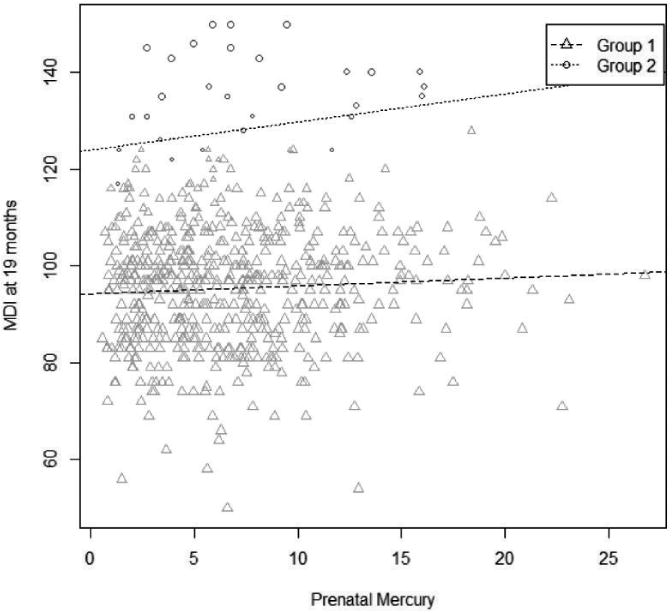
Group Membership for the LM Model with K = 2. Symbol size indicates the strength of the posterior evidence for group membership. The partial slopes estimated in the model have been back-transformed to the original scale.

The relationship between MeHg and MDI using the most likely classification into three groups for the LEM model is shown in Figure 2. The covariate estimates and posterior intervals are shown in the columns under K = 3 in Table 2. This model explains 33.18% of the variance in MDI scores. Of the nine covariates in the model, HOME score, caregiver IQ, and sex are significantly related to 19-month MDI. Two of the three LM groups have similar, non-significant scaled slopes (estimated at 0.01 and 0.09) between MeHg and MDI and significantly different scaled intercepts (estimated at −0.08 and 2.15). In the third group there is a significant beneficial effect of MeHg on intelligence (scaled slope estimated at 0.37) and a scaled intercept below the largest group (estimated at −0.36). This does not imply that MeHg is beneficial, but suggests a beneficial effect of maternal fish consumption of which MeHg is a marker.

Figure 2.

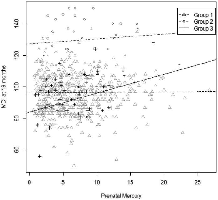
Group Membership for the LEM Model with K = 3. Symbol size indicates the strength of the posterior evidence for group membership. The partial slopes estimated in the model have been back-transformed to the original scale.

Table 2.

Parameter estimates for the LEM Model with K = 2,3,4 for Seychelles data with three SES covariates in the equation for the latent variable. The LEM model with K = 3 is preferred. The coefficients for the direct effects of the remaining covariates included zero in all models, so they are omitted here.

R2	K = 2 9.84			K = 3 33.18			K = 4 13.76
	Mean	2.5%	97.5%	Mean	2.5%	97.5%	Mean	2.5%	97.5%
HOME Score	0.25	0.11	0.38	0.19	0.09	0.29	0.21	0.08	0.34
Caregiver IQ	0.10	−0.04	0.22	0.12	0.03	0.21	0.12	0.02	0.21
Sex	−0.10	−0.17	−0.02	−0.10	−0.17	−0.03	−0.10	−0.17	−0.02
Number in Group 1	280.88	182.00	395.00	484.96	451.00	518.00	117.90	43.00	187.00
Number in Group 2	309.12	195.00	408.00	29.59	19.00	44.52	17.43	0.00	43.00
Number in Group 3				75.45	45.00	109.52	70.86	0.00	417.02
Number in Group 4							383.81	72.00	502.02
Intercept in Group 1	0.11	−0.41	0.77	−0.08	−0.17	0.02	−0.25	−0.74	0.18
Intercept in Group 2	−0.09	−0.68	0.33	2.15	1.71	2.62	1.21	−1.20	2.86
Intercept in Group 3				−0.36	−0.69	−0.00	1.04	−0.98	2.92
Intercept in Group 4							−0.04	−0.38	0.24
Mercury in Group 1	−0.01	−0.19	0.15	0.01	−0.07	0.09	0.25	0.03	0.63
Mercury in Group 2	0.11	−0.05	0.24	0.09	−0.36	0.55	0.15	−1.12	1.41
Mercury in Group 3				0.37	0.08	0.66	0.10	−1.12	1.41
Mercury in Group 4							0.02	−0.09	0.19
α Intercept for ≥2	0.18	−4.74	4.78	−3.58	−4.26	−2.65	2.84	−2.42	4.96
α Intercept for ≥3				−4.42	−4.98	−3.32	1.48	−3.67	4.57
α Intercept for ≥4							−0.62	−4.82	3.91
α HOME Score	13.06	−89.80	95.07	2.93	1.82	4.06	−9.49	−35.88	−1.69
α Caregiver IQ	−1.63	−93.25	90.44	1.30	0.40	2.21	−5.00	−20.53	−0.47
α Income Cat 1	5.11	−90.70	92.22	−0.71	−1.63	0.34	1.79	−0.26	7.97
α Income Cat 2	−63.48	−98.85	3.89	−1.59	−2.59	−0.63	8.26	0.65	46.66
α Income Cat 3	−12.95	−96.21	91.71	−2.00	−3.10	−0.80	−23.10	−93.33	2.91

Table 3 shows summary statistics for the two group fit of the LM model and the three group fit of the LEM model. Here, observations are assigned to the single group in which they have the highest posterior probability. In the LM model, subjects in group 2 have slightly higher mean values on all the variables (except sex), but the difference is only very big for MDI scores. In the LEM model, group 2 has the highest mean value on all the variables except HOME score and caregiver IQ; group 3 has the highest mean value on those two variables.

Table 3.

We assigned each child in the Seychelles data to the group where it has highest posterior probability of membership. These are summaries of the variables measured for the two LM Model groups and the three LEM Model groups.

n	The LM Model: 2 groups				The LEM Model: 3 groups
	Group 1 561		Group 2 29		Group 1 502		Group 2 26		Group 3 62
	Mean	SD	Mean	SD	Mean	SD	Mean	SD	Mean	SD
HOME Score	33.44	5.24	36.97	5.06	32.47	4.59	38.54	3.72	40.87	3.98
Caregiver IQ	23.51	10.71	26.59	9.69	22.08	9.88	28.38	9.55	34.53	10.52
Income	1.06	1.05	1.41	1.09	1.05	1.03	1.35	1.13	1.19	1.17
Sex	0.51	0.50	0.48	0.51	0.50	0.50	0.50	0.51	0.55	0.50
Mother's Age	26.08	5.75	26.72	5.99	26.19	5.87	25.68	5.29	25.71	4.97
Mother's Ed	0.47	0.68	0.69	0.71	0.46	0.70	0.65	0.69	0.52	0.54
Father's Ed	0.85	0.86	1.03	0.82	0.88	0.87	0.96	0.77	0.61	0.66
Breastfeeding Dur	0.58	0.59	0.76	0.58	0.61	0.61	0.58	0.50	0.48	0.54
Prenatal Mercury	6.75	4.50	7.58	4.57	6.77	4.54	7.35	4.37	6.68	4.30
19-month MDI	95.57	12.15	135.52	8.98	95.73	12.42	135.81	9.28	96.10	12.54

The order of the three groups in the LEM model is not arbitrary, they are ordered by the latent variable of SES which is significantly related to HOME score, caregiver IQ, and income category. The estimated latent variable has a positive relationship with HOME score and caregiver IQ (coefficients of 2.93 and 1.3) and a negative relationship with income (coefficients of −0.71, −1.59, and −2 for the three ordered levels of income compared to the lowest level). This suggests that children in higher income households require more stimulation (caregiver IQ and HOME score) in order to be as likely to get any benefit from increased prenatal fish consumption (be in the third group). Smaller fish are more expensive and tend to be at a lower trophic level (lower MeHg) than larger fish. Compared to a low SES mother, a high SES mother with the same prenatal MeHg may be eating much more fish. The earlier effect modification analysis simultaneously included interaction terms for two of the three SES variables and had R² = 14 %.² They did not find a significant interaction between prenatal methylmercury and HOME score. In contrast, in our model HOME score is a very significant predictor of group membership.

We examined the robustness of these results by refitting both models without the 22 children with the highest MDI scores (results not shown). As we might expect, the LM model finds no evidence of more than one subpopulation. Reassuringly, the LEM model shows support for two subpopulations. The latent variable distinguishing these groups is similar to that defined by α in Table 2, having a positive relationship with HOME score and caregiver IQ and a negative relationship with income. As in the full analysis, the first, larger group has a non-significant relationship between MeHg and MDI. The second, smaller group has a smaller intercept and larger slope, following the pattern of the third group in the full analysis. However, the slope is not significantly different than zero for that group. The small number of remaining children assigned to group 2 in the full LEM analysis are assigned to the second group in this analysis and they attenuate the estimated MeHg association in this group.

As a second sensitivity analysis, we focused on the two observations in the LEM model assigned to group 3 with prenatal mercury values greater than 16. These observations have large MDI values as well which make them potentially influential. We repeated the analysis without those two observations and the assignment of subjects to groups and the group-specific slopes were changed very little. We also examined several other perturbations of the data such as collapsing the four income categories into two, but the results remained very consistent with results reported above.

6 Summary

To explain the complex association between prenatal methylmercury and child's IQ as measured at 19 months in the SCDS, we compared two models for effect modification of exposure response relationships by latent variables. We fit these models within a Bayesian framework. Both models assume a linear regression relating covariates to a continuous outcome with common covariate slopes for all K latent groups, but allow group-specific intercepts and exposure slopes. In the LM model the posterior probability of group membership for an individual subject is a function of the relative size of the residuals from each group-specific line. The LEM model additionally introduces a logit model for group membership as a function of covariates. Posterior probability of group membership in the LEM model is a function of both the residuals from the group-specific lines in the outcome model and the probability of group membership in the logit model. Both LM and LEM models have multiple modes due to label-switching.

Our simulations strongly supported preferring the LEM model where exposure slopes are of primary importance or the group-specific intercepts and slopes are not large, which includes the case of the SCDS data. This model was very useful for the SCDS data example, because explicitly introducing a model for group membership as a function of multiple SES variables (the LEM model) makes it possible to examine the evidence for effect modification by a latent group, where the latent group is defined by SES. Only when we included the additional model for group membership as a function of SES variables did we find evidence for a group of subjects with a very different exposure slope.

The latent grouping variable in an LEM model creates a score for any new individual which classifies them into a group with a common exposure response relationship. Based on the data likelihood, the LEM model determines the optimum number of groups and group membership probabilities without categorizing continuous variables. This alleviates the problem of needing to interpret multiple interactions with exposure as might occur in a standard effect modification model. The LEM model may be useful in other situations when effect modification by several related covariates is hypothesized.

References

- 1.Bellinger D. Effect modification in epidemiologic studies of low-level neurotoxicant exposures and health outcomes. Neurotox Terat. 2000;22:133–140. doi: 10.1016/s0892-0362(99)00053-7. [DOI] [PubMed] [Google Scholar]
- 2.Davidson P, Myers G, Shamlaye C, et al. Association between prenatal exposure to methylmercury and developmental outcomes in Seychellois children: effect modification by social and environmental factors. Neurotox. 1999;20:833–841. [PubMed] [Google Scholar]
- 3.Hastie T, Tibshirani R. Varying-coefficient models. J R Stat Soc B. 1993;55(4):757–796. [Google Scholar]
- 4.Thompson T, Smith P, Boyle J. Finite mixture models with concomitant information: assessing diagnostic criteria for diabetes. J R Stat Soc C. 1998;47:393–404. [Google Scholar]
- 5.Dayton C, Macready G. Concomitant-variable latent-class models. J Am Stat Assoc. 1988;83:173–178. [Google Scholar]
- 6.Bandeen-Roche K, Miglioretti D, Zeger S, et al. Latent variable regression for multiple discrete outcomes. J Am Stat Assoc. 1997;92:1375–1386. [Google Scholar]
- 7.Bollen K, Bollen K. Structural equations with latent variables. Vol. 8. New York: Wiley; 1989. [Google Scholar]
- 8.Peng F, Jacobs R, Tanner M. Bayesian inference in mixtures-of-experts and hierarchical mixtures-of-experts models with an application to speech recognition. J Am Stat Assoc. 1996;91:953–960. [Google Scholar]
- 9.Gormley I, Murphy T. A mixture of experts model for rank data with applications in election studies. Stat Sci. 1992;7:457–472. [Google Scholar]
- 10.Handcock M, Raftery A, Tantrum J. Model-based clustering for social networks. J R Stat Soc A. 2007;170:301–354. [Google Scholar]
- 11.Grün B, Leisch F. FlexMix Version 2: finite mixtures with concomitant variables and varying and constant parameters. J Stat Software. 2008;28:1–35. [Google Scholar]
- 12.Frühwirth-Schnatter S. Finite mixture and Markov switching models. Vol. 423. New York: Springer; 2006. [Google Scholar]
- 13.Agresti A. An introduction to categorical data analysis. Vol. 423. Wiley-Blackwell; Hoboken, NJ: 2007. [Google Scholar]
- 14.Plummer M. JAGS: Just another Gibbs sampler. [accessed 5 June 2013];2007 https://sourceforge.net/projects/mcmc-jags.
- 15.Stephens M. Dealing with label switching in mixture models. J R Stat Soc B. 2000;62:795–809. [Google Scholar]
- 16.Davidson P, Myers G, Cox C, et al. Longitudinal neurodevelopmental study of Seychellois children following in utero exposure to methylmercury from maternal fish ingestion: outcomes at 19 and 29 months: methylmercury and human health. Neurotox. 1995;16:677–688. [PubMed] [Google Scholar]
- 17.Cernichiari E, Brewer R, Myers G, et al. Monitoring methylmercury during pregnancy: maternal hair predicts fetal brain exposure. Neurotox. 1995;16:705–710. [PubMed] [Google Scholar]
- 18.Lapham L, Cernichiari E, Cox C, et al. An analysis of autopsy brain tissue from infants prenatally exposed to methymercury. Neurotox. 1995;16:689–704. [PubMed] [Google Scholar]
- 19.Raftery A, Lewis S. One long run with diagnostics: Implementation strategies for Markov chain Monte Carlo. Stat Sci. 1992;7:493–497. [Google Scholar]
- 20.Rubin D, Stern H. Testing in latent class models: Using a posterior predictive check distribution. In: von Eye A, Clogg CC, editors. Latent variables analysis: applications for developmental research. Thousand Oaks, CA: Sage; 1994. pp. 420–438. [Google Scholar]
- 21.Rousseau J, Mengersen K. Asymptotic behaviour of the posterior distribution in overfitted mixture models. J R Stat Soc B. 2011;73:689–710. [Google Scholar]
- 22.Harrell F. Springer Series in Statistics. New York: Springer; 2002. Regression modeling strategies. [Google Scholar]
Associated Data
This section collects any data citations, data availability statements, or supplementary materials included in this article.