FEATURE SELECTION IMPROVES THE ACCURACY OF CLASSIFYING ALZHEIMER DISEASE USING DIFFUSION TENSOR IMAGES

Abstract

Diffusion tensor imaging (DTI) has recently been added to several large-scale studies of Alzheimer’s disease (AD), such as the Alzheimer’s Disease Neuroimaging Initiative (ADNI), to investigate white matter (WM) abnormalities not detectable on standard anatomical MRI. Disease effects can be widespread, and the profile of WM abnormalities across tracts is still not fully understood. Here we analyzed image-wide measures from DTI fractional anisotropy (FA) maps to classify AD patients (n=43), mild cognitive impairment (n=114) and cognitively healthy elderly controls (n=70). We used voxelwise maps of FA along with averages in WM regions of interest (ROI) to drive a Support Vector Machine. We further used the ReliefF algorithm to select the most discriminative WM voxels for classification. This improved accuracy for all classification tasks by up to 15%. We found several clusters formed by the ReliefF algorithm, highlighting specific pathways affected in AD but not always captured when analyzing ROIs.

1. INTRODUCTION

Alzheimer’s disease (AD), a debilitating neurodegenerative disorder that affects the elderly, is the most common type of dementia worldwide. Pathological changes related to AD may begin decades before clinical symptoms are detected, and methods are needed to help predict who will ultimately be diagnosed with AD and who is most likely to show imminent cognitive decline. Mild cognitive impairment (MCI) is a state of abnormal cognitive function intermediate between healthy aging and AD, and around 10–15% of people with MCI convert to dementia every year [1, 2].

Diffusion tensor imaging (DTI) of the brain may help in distinguishing stages of AD by evaluating white matter (WM) alterations, including myelin breakdown and axonal loss [3–6]. DTI measures water diffusion in brain tissue and provides various measures of microstructural integrity and pathology [4]. Numerous DTI studies show white matter differences between AD and normal control (NC) [3–11]. Even with healthy aging, DTI changes over time are detectable in the frontal WM, anterior cingulum and the genu of the corpus callosum. In AD, abnormalities tend to be more severe, primarily in posterior regions; the parahippocampal gyrus, temporal WM, splenium of corpus callosum and posterior cingulum. In MCI, changes resemble those in AD, with similar but lesser abnormalities in posterior regions [3].

Patients with AD can be differentiated, with varying degrees of accuracy, from people with MCI and NC using machine learning techniques. Support vector machines (SVM) have been used successfully in AD and MCI studies. Dyrba et al. [9] used DTI indices FA and mean diffusivity (MD) with SVM to classify 137 people as AD or NC. They selected voxels to improve classification performance, using Plant’s approach [10] and an “information gain” criterion. They achieved an accuracy of 80% for classifications based on FA, and 83% for MD. Haller et al. [11] measured FA, axial, radial, and mean diffusivity in 35 NC and 67 MCI subjects using Tract Based Spatial Statistics. They performed classification of MCI cases versus controls, using SVM and obtained up to 91.4% accuracy. Nir et al. [12] performed a SVM based classification of AD using DTI measures interpolated along the maximum density paths based on whole-brain tractography. They obtained 74.5% accuracy for AD vs NC using FA and 80.6% using MD; of course, these results depend on the age and scan quality of the cohort assessed, and whether patients have other co-morbid conditions. Even so, they suggest the utility of DTI for AD research.

Here we took an unbiased brain-wide approach to identify voxels and regions in FA images that best discriminate between AD, MCI and NC in both voxelwise and ROI analyses. We compared the classification accuracy between averaged ROI features, voxels throughout the WM, and voxels selected by the ReliefF algorithm by applying SVM to data from 221 ADNI participants. We applied 10 times 10-fold cross validation for feature selection and classification, to assess the generalizability of the performance.

2. MATERIALS AND METHODS

2.1. Demographics and DTI Scans

DWI scans, clinical, and neuropsychological data were downloaded from the ADNI database (http://adni.loni.usc.edu) and we performed a cross-sectional analysis of 211 participants scanned at 14 data acquisition sites (70 NC, 114 MCI and 37 AD patients). Cognitive evaluations of each subject included the Mini-Mental State Examination (MMSE), the “sum-of-boxes” Clinical Dementia Rating (CDR-sob) and the Alzheimer's Disease Assessment Scale-Cognitive (ADAS-cog) [4]. Demographics and mean test scores for the participants are given in Table 1. As expected, diagnostic groups differed significantly in cognitive test scores.

Table 1.

Demographics and mean test scores.

	AD	MCI	Normal
Size	37	114	70
Female/Male	17/20	45/69	39/31
Age (Mean±SD)	75.1±8.7	71.9±7.7	72.3±5.6
MMSE (Mean±SD)	23.4±1.9	27.8±1.7	28.9±1.4
CDR-sob	4.6±1.5	1.4±0.8	0.0±0.1
ADAS-cog	29.3±9.6	15.7±7.2	9.8±5.3

Diffusion weighted images (DWI) were collected with a 128 × 128 matrix, 2.7 × 2.7 × 2.7 mm³ voxel size, TR = 9000 ms, scan time, 9 min. 5 T2-weighted images with no diffusion sensitization (b=0 images) and 41 diffusion-weighted images (b=1000 s/mm²) were acquired for each DTI slice on 3-Tesla GE Medical Systems scanners at 14 acquisition sites across North America.

2.2. Image Processing

Images were processed as in [12]. Briefly, DWI volumes were corrected for eddy current distortions and echo-planar imaging (EPI) induced susceptibility artifacts by mapping to the high-resolution T1-weighted image. Gradient directions were corrected, before tensor calculations.

FSL’s dtifit was used to model a diffusion tensor at each voxel from the corrected DWI scans. Diffusion tensor eigenvalues (λ₁, λ₂, λ₃) were used to obtain scalar anisotropy and diffusivity maps. Once eigenvalues are calculated in each voxel several diffusion metrics can be calculated. The most widely used metric of diffusion anisotropy is fractional anisotropy (FA). FA is scaled from 0-isotropic to 1-anisotropic. FA is calculated using Eq. 1 and Eq. 2 (which is the equation for mean diffusivity or MD).

$$FA=\sqrt{\frac{3}{2}}\frac{\sqrt{{({\lambda }_1-\langle \lambda \rangle )}^2+{({\lambda }_2-\langle \lambda \rangle )}^2+{({\lambda }_3-\langle \lambda \rangle )}^2}}{\sqrt{{\lambda }_1^2+{\lambda }_2^2+{\lambda }_3^2}}\in [0,1]$$ (1)

$$\langle \lambda \rangle =\frac{{\lambda }_1+{\lambda }_2+{\lambda }_3}{3}$$ (2)

To extract regions of interest (ROIs), the FA image from the Johns Hopkins University (JHU) DTI atlas was registered linearly then elastically to the FA image of each individual subject, using mutual information-based registration. We used nearest neighbor interpolation to apply that deformation to the stereotaxic JHU “Eve” atlas WM labels. We then superimposed the atlas ROIs into the same coordinate space as our results. This process is detailed in [4]. We removed 10 ROIs from the analyses as they often fell partially or completely out of the field-of-view (FOV) of the images. We also excluded the body of the fornix as it is small and prone to misregistration and partial voluming. We included the crus of the fornix/stria terminalis and bilateral genu, body, and splenium of the corpus callosum as well as the entire corpus callosum, and a large “TOTAL” WM ROI made up of all the other ROIs, to obtain total summary measures of these regions in addition to the JHU labels. We then calculated average FA within the boundaries of ROIs for each subject. Visual quality control ensured all ROIs were suitably overlaid on the FA image and adequate for statistical analysis. All our ROI summary measures from the JHU template are available at the ADNI website (adni.ini.usc.edu).

For our voxelwise analysis, we first made a population atlas from the FA maps and registered all subjects to it, so that voxels corresponded as far as possible across all scans. First, a minimal deformation template (MDT) was created using spatially aligned FA maps from 29 healthy controls then registering all the individual scans to that template using a fluid registration while regularizing the Jacobians [13]. A new mean was created from the registered scans; this process was iterated several times. Each subject's initial FA map was elastically registered to the final MDT using a mutual information driven algorithm. To ensure further WM alignment across subjects, registered FA maps were thresholded at FA > 0.2 to include only highly anisotropic anatomy and the thresholded maps were once again registered to the thresholded MDT (FA > 0.2).

2.3. Feature Selection

Without using a priori information on the regions known to relate to disease, we first aimed to select a subset of WM voxels that would be most helpful for classification of AD, MCI and NC groups, for dimensionality reduction. Feature selection may boost the accuracy of a classifier by excluding voxels that do not contribute to distinguishing between groups. It also decreases the computation time.

The spatially aligned FA maps contain 110 × 110 × 110 voxels. However, of the 12,100 voxels per slice and 1,331,000 voxels overall, only 49,034 fell within the WM and were therefore appropriate to use as features from DTI images. We used three different types of input for classification; 115 features that correspond to FA averages in ROIs described in section 2.2, all 49,034 WM voxels of the FA maps, and features selected among the WM voxels using the ReliefF algorithm [14–16]. The ReliefF algorithm estimates the quality of inputs by using k-nearest neighbors per class. It uses the L1 norm to find the neighbors from the same class (near-hit) and from the other class (near-miss) and updates the weight vector of each feature to find the feature’s contribution to the classification. For all three classification tasks, we selected gradually 500, 1000, 1500, 2000 and 2500 voxels that have the most power to differentiate the diagnostic groups, using the ReliefF algorithm.

2.4. Support Vector Machines

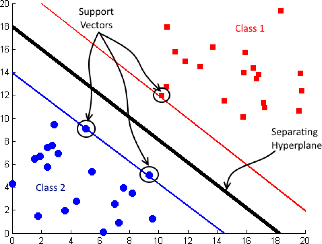
A support vector machine (SVM) is a binary classification algorithm used widely in neuroimaging, as well as for many other classification tasks [2, 9, 11, 12]. SVM is a supervised classifier that takes into account labeled training samples to learn class differences [17, 18]. SVM maps input vectors to a very high-dimensional feature space in a nonlinear fashion. A decision surface is constructed in this feature space to separate the training data in to two classes by using a separating hyperplane. A hyperplane for a linear classifier can be expressed as w^Tx + b = 0, where w is the weight vector and b is the bias for the input vector x. The decision surface is determined by the support vectors that are informative subsets of the training data. SVM maximizes the margin between support vectors by minimizing ‖w‖. Two subspaces obtained after training then correspond to the two classes (Fig. 1).

Fig. 1.

Support vectors and decision surface.

We used a sequential minimal optimization (SMO) learning algorithm with a Gaussian radial basis function (RBF) kernel to train the SVM. The Gaussian RBF kernel can be expressed as Eq. 3 [17, 18].

$$K(x,x\prime )=\text{exp}(-\frac{{\Vert x-x\prime \Vert }^2}{2{\sigma }^2})$$ (3)

SVM with an RBF kernel has two primary parameters to be set: σ, the width of the RBF function; and C, the regularization parameter for soft-margin SVM. Small C values tend to produce a large margin, while C=∞ leads to a hard margin [19, 20].

3. RESULTS AND DISCUSSION

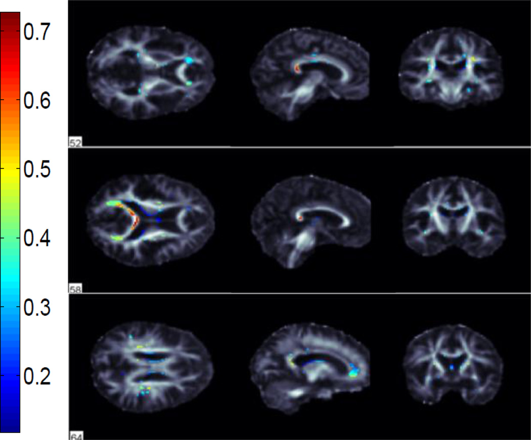
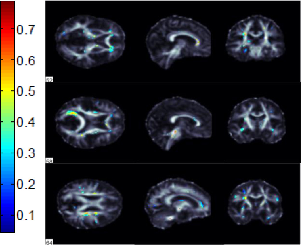
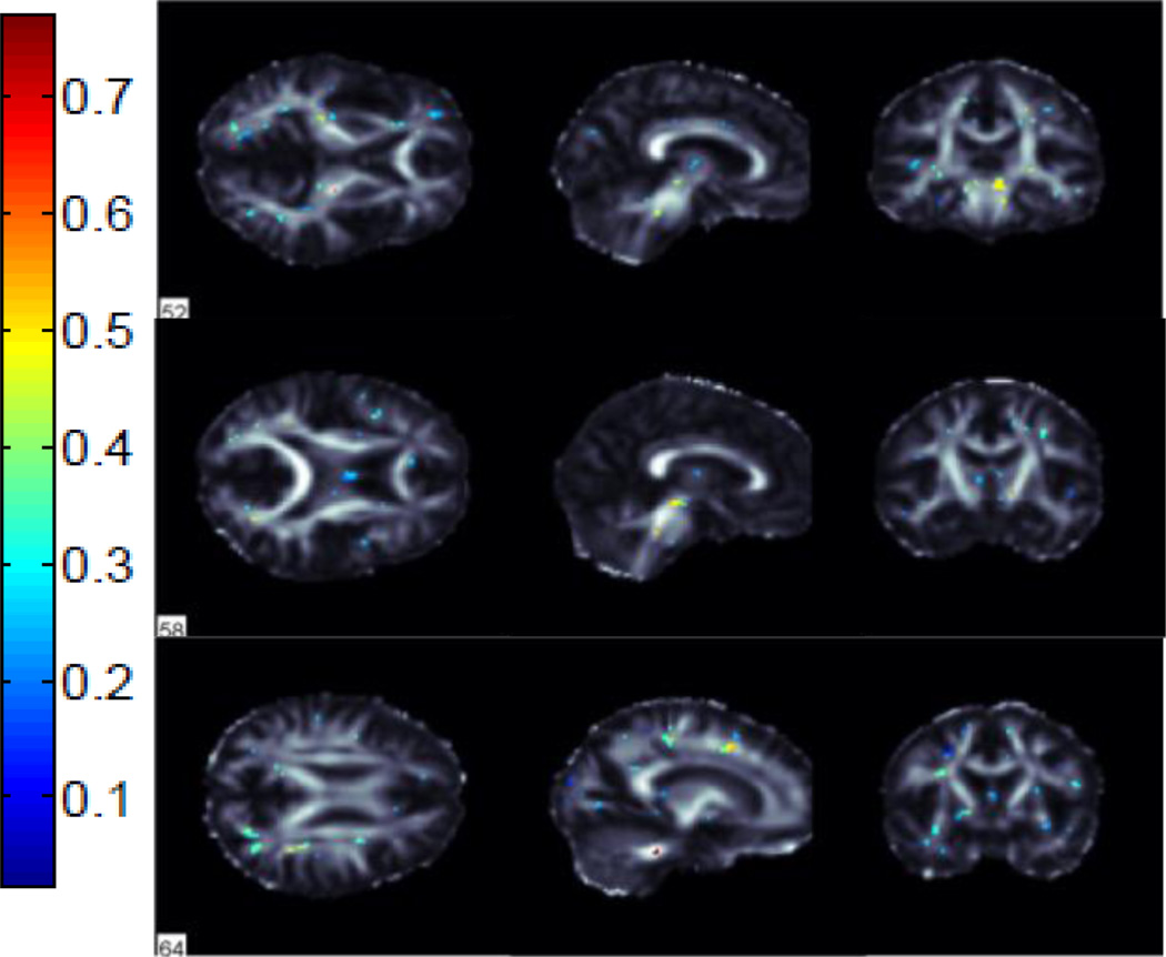
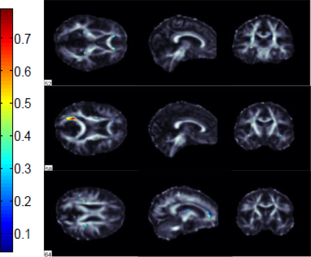
We performed classification between AD vs NC, AD vs MCI and MCI vs NC groups using FA images from 221 subjects in ADNI. We used 115 average ROI values, whole WM voxels (49,034 in total) and a subset of these WM voxels selected by the ReliefF algorithm. Using the ReliefF algorithm, we selected 500, 1000, 1500, 2000 and 2500 most important WM voxels for classification to show the effect of selecting different numbers of features. Fig. 2 shows the most important voxels selected for AD vs NC classification. Colors indicate the importance of the selected voxels. Selected voxels are in regions that typically show differences between healthy aging and AD: the anterior and posterior cingulum, genu and splenium of the corpus callosum and frontal and temporal WM. Fig. 3 and Fig. 4 show the selected WM voxels for AD vs MCI, and MCI vs NC classification, respectively. The most important voxel for classifying AD vs MCI was similar to those for classifying AD vs NC. 1/3 of the selected WM voxels for AD vs MCI and AD vs NC classification tasks overlapped (Fig. 5). Overlapping voxels were at the same locations where AD-related WM abnormalities tend to occur. However, the voxels selected for MCI vs NC classification were more scattered across the WM voxels.

Fig. 2.

Selected WM voxels for AD vs NC classification.

Fig. 3.

Selected WM voxels for AD vs MCI classification.

Fig. 4.

Selected WM voxels for MCI vs NC classification.

Fig. 5.

Overlapping voxels that were selected for both AD vs NC and AD vs MCI classification.

We employed the Gaussian RBF kernel and SMO learning function for SVM. A parameter search for the two parameters of the RBF kernel, C and σ, should be performed to ensure the prediction strength of the SVM. We selected the best parameter set by applying a grid search with 10 times 10-fold cross validation to reduce the selection-related bias. We first tried exponentially growing values of C=[2⁻⁹,2⁻⁸, …, 2¹⁵] and σ=[2⁻⁵,2⁻⁴, …, 2¹⁵] to generate a coarse grid. We then performed a finer grid search after identifying a better region on the coarse grid [21]. The best σ and C values obtained from grid search were applied to the whole training data. Training and test data points are centered at their mean, and scaled to have unit standard deviation before training. Mean-centering was performed by subtracting the mean value of each variable from the data, so that all features are centered at zero. Then the data is divided by the standard deviation of features to scale it. This is a necessary preprocessing step because otherwise the objective function of SVM might be dominated by features with have larger variances.

We evaluated our results in terms of their accuracy, sensitivity and specificity. Average classification accuracies for all three tasks for different input types are given in Table 2. We reached 92.9% specificity and 79.5% sensitivity for AD vs NC, 89.4% specificity and 77.0% sensitivity for AD vs MCI classification. Sensitivity and specificity for MCI vs NC classification were 86.2% and 65.7%, respectively. Using all the WM voxels instead of the “average ROI” features increased classification accuracies for AD vs NC and AD vs MCI classifications but had no detectable effect on MCI vs NC classification. Selecting the most important WM voxels using the ReliefF algorithm improved classification accuracies for all tasks up to 14.9%.

Table 2.

Average classification accuracies with different features

Features/Classes	AD vs NC	AD vs MCI	MCI vs NC
Average ROI	75.45%	72.66%	63.57%
Whole WM	80.76%	73.89%	63.57%
Relieff500	84.24%	82.75%	78.42%
Relieff1000	85.98%	85.26%	77.89%
Relieff1500	87.80%	85.34%	78.48%
Relieff2000	86.89%	85.93%	77.40%
Relieff2500	86.06%	82.63%	75.23%

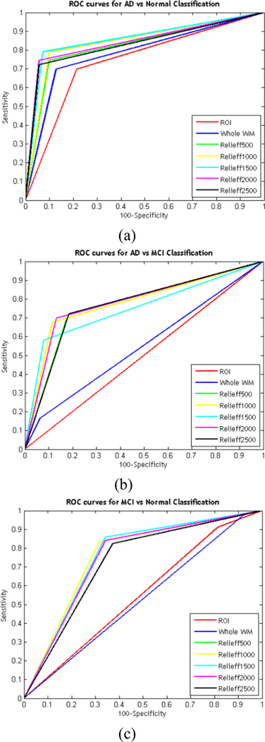
Receiver Operating Characteristic (ROC) curves for the classification tasks are shown in Fig. 6. The area under the curve (AUC) was 86.0%, 78.3% and 75.8% for AD vs NC, AD vs MCI and MCI vs NC, respectively.

Fig. 6.

ROC curves for (a) AD vs NC, (b) AD vs MCI and (c) MCI vs NC classification.

4. CONCLUSION

Interestingly, our analysis found that after AD is diagnosed, there is no detectable difference between selecting a subset of features or the entire WM, perhaps because so many voxels show a difference. However, when individually comparing NC or AD to the intermediate stage of MCI, detection is greatly improved when there is a focus on selected regions of the brain.

REFERENCES

- 1.Jack CR, et al. The Alzheimer's disease neuroimaging initiative (ADNI): MRI methods. J. Magn. Reson. Imaging. 2008;27(4):685–691. doi: 10.1002/jmri.21049. [DOI] [PMC free article] [PubMed] [Google Scholar]
- 2.O'Dwyer L, et al. Using support vector machines with multiple indices of diffusion for automated classification of mild cognitive impairment. PLoS One. 2012;7(2):e32441. doi: 10.1371/journal.pone.0032441. [DOI] [PMC free article] [PubMed] [Google Scholar]
- 3.Chua TC, Wen W, Slavin MJ, Sachdev PS. Diffusion tensor imaging in mild cognitive impairment and Alzheimer's disease: a review. Curr. Opin. Neurol. 2008;21(1):83–92. doi: 10.1097/WCO.0b013e3282f4594b. [DOI] [PubMed] [Google Scholar]
- 4.Nir TM, Jahanshad N, Villalon-Reina JE, Toga AW, Jack CR, Weiner MW, Thompson PM. Effectiveness of regional DTI measures in distinguishing Alzheimer's disease, MCI, and normal aging. NeuroImage: Clinical. 2013;3:180–195. doi: 10.1016/j.nicl.2013.07.006. [DOI] [PMC free article] [PubMed] [Google Scholar]
- 5.Oishi K, Mielke MM, Albert M, Lyketsos CG, Mori S. DTI analyses and clinical applications in Alzheimer's disease. J. Alzheimers Dis. 2011;26:287–296. doi: 10.3233/JAD-2011-0007. [DOI] [PMC free article] [PubMed] [Google Scholar]
- 6.Bozzali M, et al. White matter damage in Alzheimer's disease assessed in vivo using diffusion tensor magnetic resonance imaging. J. Neurol. Neurosur. Ps. 2002;72(6):742–746. doi: 10.1136/jnnp.72.6.742. [DOI] [PMC free article] [PubMed] [Google Scholar]
- 7.Jahanshad N, et al. IEEE Int. Symp. on Biomedical Imaging: From Nano to Macro. Rotterdam: 2010. Diffusion tensor imaging in seven minutes: determining trade-offs between spatial and directional resolution; p. 1161.p. 1164. [Google Scholar]
- 8.Newlander SM, Chu A, Sinha US, Lu PH, Bartzokis G. Methodological improvements in voxel-based analysis of diffusion tensor images: Applications to study the impact of apolipoprotein E on white matter integrity. J. Magn. Reson. Imaging. 2014;39(2):387–397. doi: 10.1002/jmri.24157. [DOI] [PMC free article] [PubMed] [Google Scholar]
- 9.Dyrba M, et al. Robust automated detection of microstructural white matter degeneration in Alzheimer’s disease using machine learning classification of multicenter DTI data. PLoS One. 2013;8(5):e64925. doi: 10.1371/journal.pone.0064925. [DOI] [PMC free article] [PubMed] [Google Scholar]
- 10.Plant C, et al. Automated detection of brain atrophy patterns based on MRI for the prediction of Alzheimer’s disease. NeuroImage. 2010;50:162–174. doi: 10.1016/j.neuroimage.2009.11.046. [DOI] [PMC free article] [PubMed] [Google Scholar]
- 11.Haller S, et al. Individual prediction of cognitive decline in mild cognitive impairment using support vector machine-based analysis of diffusion tensor imaging data. J. Alzheimers Dis. 2010;22(1):315–327. doi: 10.3233/JAD-2010-100840. [DOI] [PubMed] [Google Scholar]
- 12.Nir TM, et al. Diffusion weighted imaging-based maximum density path analysis and classification of Alzheimer's disease. Neurobiol. Aging. 2015;36:S132–S140. doi: 10.1016/j.neurobiolaging.2014.05.037. [DOI] [PMC free article] [PubMed] [Google Scholar]
- 13.Gutman B, et al. Creating unbiased minimal deformation templates for brain volume registration. Proc. of the Organization for Human Brain Mapping Annu. Conf.; Barcelona. 2010. [Google Scholar]
- 14.Kira K, Rendell LA. Proc. of the 9th Int. Workshop on Machine Learning. Aberdeen: 1992. A practical approach to feature selection; p. 249.p. 256. [Google Scholar]
- 15.Kira K, Rendell LA. The feature selection problem: Traditional methods and a new algorithm. Proc. of the 10th Nat. Conf. on Artificial Intelligence; San Jose, CA. 1992. p. 129.p. 134. [Google Scholar]
- 16.Kononenko I, Simec E, Robnik-Sikonja M. Overcoming the myopia of inductive learning algorithms with RELIEFF. Appl. Intell. 1997;7:39–55. [Google Scholar]
- 17.Vert JP, Tsuda K, Schölkopf B. Kernel Methods in Computational Biology. Vol. 2. MIT Press; 2004. A primer on kernel methods; pp. 35–70. [Google Scholar]
- 18.Burges CJ. A tutorial on support vector machines for pattern recognition. Data Min. Knowl. Disc. 1998;2(2):121–167. [Google Scholar]
- 19.Cortes C, Vapnik V. Support-vector networks. Mach. Learn. 1995;20:273–297. [Google Scholar]
- 20.Magnin B, et al. Support vector machine-based classification of Alzheimer’s disease from whole-brain anatomical MRI. Neuroradiology. 2009;51(2):73–83. doi: 10.1007/s00234-008-0463-x. [DOI] [PubMed] [Google Scholar]
- 21.Hsu C-W, Chang C-C, Lin C-J. A practical guide to support vector classification. Department of Computer Science, National Taiwan University, Taipei, Taiwan, Tech. Rep.; 2003. [Google Scholar]