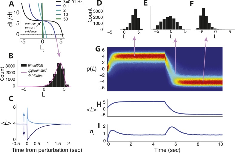
(
A) Example of the temporal derivative of belief magnitude plotted as a function of belief magnitude (
Equation 4), given an average sensory evidence of 7 units of
LLR per unit time. The point of intersection with the dotted line (i.e., derivative = 0) corresponds to the approximate steady-state value of the belief (the mode of the probability distribution). (
B) Histogram of belief values at steady state for hazard rate λ = 0.1 Hz from panel
A, with the approximated solution in
Equation 14a shown in magenta. Note the heavy tail, which is typical for moderate-to-strong input to the model. (
C) Asymmetric effects of transient ‘perturbations’ of evidence of equal magnitude (35 units of
LLR per s) but opposite signs. Belief magnitude re-converges to steady state faster after the positive perturbation (i.e., favoring the current belief) than the negative perturbation (i.e., opposing the current belief), which accounts for the heavy tail pointed towards zero in
B. (
D–
I) Simulated temporal evolution of the probability distribution of belief value, given an average sensory evidence of 7 units of
LLR per s, with an abrupt sign reversal at
t = 5 s. (
D–
F) Histograms of belief at the time-points indicated by arrows. (
G) Pseudocolor plot of the full probability distributions normalized by the peak probability over the entire time series. Hot/cold colors indicate high/low probabilities. (
H) Expected value of the belief variable. (
I) Standard deviation of the belief variable. Note that after a change-point, leaky integration is re-started and beliefs pass through the ‘low-confidence’ regime of the model, resulting in a transient increase of variability that is approximately Gaussian. All simulations used 10,000 iterations.


