

Abstract
The precise delineation of auditory areas in vivo remains problematic. Histological analysis of postmortem tissue indicates that the relation of areal borders to macroanatomical landmarks is variable across subjects. Furthermore, functional parcellation schemes based on measures of, for example, frequency preference (tonotopy) remain controversial. Here, we propose a 7 Tesla magnetic resonance imaging method that enables the anatomical delineation of auditory cortical areas in vivo and in individual brains, through the high-resolution visualization (0.6 × 0.6 × 0.6 mm3) of intracortical anatomical contrast related to myelin. The approach combines the acquisition and analysis of images with multiple MR contrasts (T1, T2*, and proton density). Compared with previous methods, the proposed solution is feasible at high fields and time efficient, which allows collecting myelin-related and functional images within the same measurement session. Our results show that a data-driven analysis of cortical depth-dependent profiles of anatomical contrast allows identifying a most densely myelinated cortical region on the medial Heschl's gyrus. Analyses of functional responses show that this region includes neuronal populations with typical primary functional properties (single tonotopic gradient and narrow frequency tuning), thus indicating that it may correspond to the human homolog of monkey A1.
Keywords: auditory cortex, cortical myelin-related contrast, high-field MRI, tonotopy
Introduction
Despite extensive research, the objective identification of auditory areas in individual subjects by non-invasive anatomical or functional imaging remains challenging. Cytoarchitectural studies of postmortem brains indicate that, in humans, the primary auditory cortex proper (A1) is situated on the medial portion of the Heschl's gyrus (HG) and is neared by primary-like areas so as to form a cortical core (Hackett et al. 2001). This primary core is surrounded by a number of non-primary belt and parabelt regions (Celesia 1976; Galaburda and Sanides 1980; Rivier and Clarke 1997). The position of A1 relative to sulcal and gyral landmarks is variable (Penhune et al. 1996; Morosan et al. 2001; Rademacher et al. 2001). Moreover, while tonotopic maps (reflecting the frequency preference of auditory neuronal populations) can be obtained in vivo using functional magnetic resonance imaging (fMRI; Formisano et al. 2003; Striem-Amit et al. 2011), their interpretation with regard to the precise definition of A1 and other areas remains an issue of debate (Humphries et al. 2010; Striem-Amit et al. 2011; Langers and van Dijk 2012; Moerel et al. 2012). Consequently, neither macroanatomical nor functional measures suffice for accurately delineating human A1 in individual subjects. Unfortunately, the most reliable way to determine the location of A1 in a specific brain is through postmortem cytoarchitectonic or myeloarchitectonic (the Vogt–Vogt school of myeloarchitectonics; see Nieuwenhuys 2013) analysis of that brain. Even more problematic and controversial is the delineation of auditory cortical areas other than A1.
MR has been proposed to measure cortical myelination in vivo (Clark et al. 1992; Barbier et al. 2002; Walters et al. 2003). Intracortical contrast related to myelin has been mapped in vivo, at both conventional (3 Tesla; [3T]) and high (7 Tesla; [7T]) fields (Sigalovsky et al. 2006; Bock et al. 2009; Barazany and Assaf 2011; Bock et al. 2011; Geyer et al. 2011; Glasser and Van Essen 2011; Bock et al. 2013; Cohen-Adad et al. 2012; Dick et al. 2012). Variations in signal intensities within the gray matter (i.e., myelin sensitivity) have been observed using quantitative T1 mapping (Sigalovsky et al. 2006; Barazany and Assaf 2011; Geyer et al. 2011; Dick et al. 2012; Sereno et al. 2013), T1-weighted (Clark et al. 1992; Barbier et al. 2002; Walters et al. 2003; Clare and Bridge 2005), T2-weighted (Yoshiura et al. 2000; Carmichael et al. 2006; Trampel et al. 2011), quantitative T2* (Fukunaga et al. 2010; Cohen-Adad et al. 2012; Cohen-Adad 2013), and T2*-weighted images (Hinds et al. 2008; Zwanenburg et al. 2011; Sanchez-Panchuelo et al. 2012). A recent study has taken advantage of the fact that heavily myelinated areas have high signal intensities in T1-weighted images and low signal intensities in T2-weighted images, which results in ratio images (T1w/T2w) that have not only enhanced contrast (Glasser and Van Essen 2011), but also have partially reduced sensitivity to undesirable signal variations from radio-frequency (RF) transmit or receive profiles.
While high-resolution (i.e., submillimeter) in vivo myeloarchitectonic mapping has been achieved at both 3T (Dick et al. 2012; Glasser et al. 2013) and 7T (Geyer et al. 2011), a critical limiting factor has been the ability to obtain whole-brain high-resolution functional and anatomical images within a reasonable acquisition time and with sufficient sensitivity. Both high spatial resolution and reduced acquisition time are necessary elements for enabling meaningful investigations of the relation between microstructural and functional architecture in the human brain. In fact, high spatial resolution isotropic acquisitions are necessary because of the folded nature of the cortical ribbon and the relatively small thickness of myelinated areas (Geyer et al. 2011; Dick et al. 2012; Zilles and Amunts 2012; Glasser et al. 2013). Reduced acquisition times are not only favorable for reducing the impact of subject motion, but also provide the possibility to perform functional measurements in the same subject and in the same measurement session, which is optimal for studying the relation between anatomy and function.
At high fields (7T), functional and anatomical contrasts are intrinsically enhanced (Duyn et al. 2007; Abosch et al. 2010), which make it possible to image brain structures at submillimeter isotropic resolutions in individual subjects and across the entire brain. However, collecting whole-brain (anatomical) data at high fields represents a challenge and localized high-resolution and -sensitivity functional images have been the primary attractors to high field imaging. Signal intensity biases due to RF transmit and receive profiles are among the primary reasons for this. The use of ratio images has been shown to provide more uniform T1 contrast (van de Moortele et al. 2009), and, for the most part, circumvent this limitation. In principle, ratio images (T1w/T2w) could also be used at 7T to obtain enhanced myelin-related contrast, similar to 3T (Glasser and Van Essen 2011). However, collecting whole-brain T2-weighted images at 7T is prohibitive due to both inhomogeneous transmit profiles and power deposition limitations. As such, if feasible, T2*-weighted images would be a much more attractive option for whole-brain high-resolution imaging of intracortical features at 7T (Cohen-Adad 2013). Importantly, several factors have been shown to contribute to the tissue T2*, most prominently myelin and iron. Because iron and myelin are colocalized in the cortex, this contrast can be used to study cortical myelination (Fukunaga et al. 2010; Cohen-Adad 2013).
The aim of this article is 2-fold. First, we build on the idea of ratio images at 7T (van de Moortele et al. 2009) and propose a time-efficient method that—through the combination of different MR contrast mechanisms (T1, T2*, and proton density [PD])—allows visualizing anatomical contrast (T1w/T2*w) related to myelin at high spatial resolution in vivo and in individual subjects. Secondly, we illustrate its application through a detailed analysis of the relation between microstructural and functional properties of the auditory cortex. As A1 is more densely myelinated than surrounding regions (Hackett et al. 2001), the T1w/T2*w contrast may provide the required information for its accurate delineation in vivo. Recently, initial evidence for this hypothesis has been obtained combining 3T anatomical data with 1.5 T functional measures (Dick et al. 2012). Here, we use high-resolution 7T MRI and show that the cortical depth-dependent variation of T1w/T2*w contrast allows delineating human area A1 and parcellating other temporal lobe areas. Furthermore, we exploit the temporal efficiency of our approach by recording fMRI time series within the same sessions as the anatomical acquisitions. The joint analysis of anatomical data and fMRI data validates our conclusion by showing that the cortical region with the highest T1w/T2*w on the HG overlaps with neuronal populations with typical primary functional properties (tonotopy, narrow frequency tuning).
Materials and Methods
Six subjects (median age = 32, 4 males) with self-reported normal hearing participated in a first session, where anatomical and functional images were acquired to map T1w/T2*w contrast and tonotopy (based on “tones”; see below), respectively. Three of these subjects additionally took part in a second session (2 males), during which functional responses to natural sounds were measured (“natural sounds”; see below). The imaging protocol used in this study was approved by the Institutional Review Board (IRB) of the University of Minnesota.
Anatomical Data Acquisition
Data were acquired on a Siemens 7T whole body system driven by a Siemens console. A head RF coil (Nova Medical; single transmit [circularly polarized mode], 24 receive channels) was used to acquire anatomical and functional (T2*-weighted blood oxygen level-dependent) images. In the first session, we acquired 2 T1-weighted (0.6 mm isotropic) scans using a magnetization-prepared rapid acquisition gradient-echo (MPRAGE) sequence (repetition time [TR] = 3100 ms; time to inversion [TI] = 1500 ms [adiabatic non-selective inversion pulse]; (Garwood and Ugurbil 1992); time echo [TE] = 3.5 ms; flip angle = 5°; generalized autocalibrating partially parallel acquisitions [GRAPPA] = 3 (Griswold et al. 2002); FOV = 229 × 229 mm; matrix size = 384 × 384; 256 slices; pixel bandwidth = 180 Hz/pixel; first phase encode direction anterior to posterior; second phase encode direction left to right), one PD image (0.6 mm isotropic) with the same MPRAGE as for the T1-weighted image but without the inversion pulse (TR = 2160 ms; TE = 3.5 ms; flip angle = 5°; GRAPPA = 3 (Griswold et al. 2002); FOV = 229 × 229 mm; matrix size = 384 × 384; 256 slices; pixel bandwidth = 180 Hz/pixel; first phase encode direction anterior to posterior; second phase encode direction left to right), and one T2*-weighted anatomical image (0.6 mm isotropic) using a modified MPRAGE sequence that allows freely setting the TE (TR = 4910 ms; TE = 16 ms; flip angle = 8°; GRAPPA = 3 (Griswold et al. 2002); FOV = 229 × 229 mm; matrix size = 384 × 384; 256 slices; pixel bandwidth = 480 Hz/pixel; first phase encode direction anterior to posterior; second phase encode direction left to right). TE used in the T2*-weighted anatomical images was optimized in one subject by acquiring multiple TEs and choosing the image that resulted in the strongest T1w/T2*w intracortical contrast while not exhibiting excessive artifacts in lower frontal areas. Magnetic field inhomogeneities near the sinus cavity make imaging in these locations problematic. This can result in image artifacts, increased distortions, or resolution loss. The acquisition time for all the anatomical images in session 1 was approximately 25 min.
In the second session, we acquired one T1-weighted dataset (1 mm isotropic) for the purpose of alignment of functional data within session and alignment across sessions. We used an MPRAGE sequence for the acquisition of T1-weighted (TR = 3000 ms; TI = 1500 ms [adiabatic non-selective inversion pulse] (Garwood and Ugurbil 1992); TE = 4.29 ms; flip angle = 4°; GRAPPA = 3 (Griswold et al. 2002); FOV = 232 × 256 mm; matrix size = 232 × 256; 176 slices; pixel bandwidth = 140 Hz/pixel; first phase encode direction anterior to posterior; second phase encode direction left to right) and PD images (one per subject; 1 mm isotropic; TR = 2370 ms; TE = 4.29 ms; flip angle = 4°; GRAPPA = 3; (Griswold et al. 2002); FOV = 232 × 256 mm; matrix size = 232 × 256; 176 slices; pixel bandwidth = 140 Hz/pixel; first phase encode direction anterior to posterior; second phase encode direction left to right).
Anatomical Data Analysis
All analyses of the anatomical data were performed using custom Matlab code and BrainVoyager QX (Brain Innovation, The Netherlands).
Figure 1 illustrates the proposed MR imaging acquisition and processing pipeline. To correct for subject motion in between acquisitions, we aligned the anatomical data (T1w, PDw, and T2*w) by using the automatic alignment routine as implemented in BrainVoyager QX. To remove signal intensity biases related to the transmit and receive profiles of the RF coil (see original data in Fig. 1, top row), we divide T1w by PDw images (T1w/PDw), producing anatomical images with high contrast between gray and white matter (van de Moortele et al. 2009; Fig. 1, second row). Similarly, we divide T1w by T2*w images (T1w/T2*w) to enhance intracortical anatomical contrast while reducing low spatial frequency biases due to receive and transmit profiles (Fig. 1, second row). Finally, the ratio of PDw and T2*w images, while reducing the white/gray matter contrast, enhanced contrast between veins and the brain (Fig. 1, second row). Anatomical images were further corrected for residual inhomogeneities (IIHC) (see Supplementary Material for details). All ratio images are then resampled to Talairach space to allow the use of standard segmentation algorithms (e.g., as implemented in BrainVoyager QX) and intersubject alignment using the information of the cortical folding pattern (Goebel et al. 2006). The border between gray and white matter was obtained by segmenting the T1w/PDw images (Fig. 1, third row). The segmented anatomical data were inspected and manually edited in order to produce accurate results. After the segmentation of the cortical ribbon and the computation of cortical thickness (Jones et al. 2000), we defined 9 equidistant surfaces within the cortical ribbon representing the evolution of the white/gray matter boundary at distinct relative cortical depths (Polimeni et al. 2010; Khan et al. 2011; Fig. 1, bottom row; see Supplementary Material for details). The definition of surfaces at different relative cortical depths represents an approximation to the real location of the cortical laminae (Waehnert et al. 2014). Defining 9 (or more) equidistant surfaces was previously demonstrated to be valuable for visualizing the variation of intracortical anatomical (and functional) contrast (see, e.g., Polimeni et al. 2010; Dick et al. 2012). The anatomical contrast in the cortical ribbon was obtained from the T1w/T2*w data after removal of large superficial and cortical veins (i.e., by thresholding the individual's venograms obtained from PDw/T2*w, voxels exceeding the defined threshold were removed from the volumetric maps of intra T1w/T2*w contrast) by linearly rescaling the contrast values in the [1–10] range. Resulting cortical maps were projected on the individual cortical surfaces averaging the contribution throughout the cortical ribbon or on all 9 depth-dependent meshes. The depth-dependent T1w/T2*w contrast was submitted to a clustering (k-means; N = 7 clusters; repeated n = 100 times with random initialization for each subject) procedure resulting in a parcellation (i.e., a spatial map and a cluster centroid representing the average of all vertices belonging to that cluster) in each individual subject (Fig. 1). This analysis was limited to vertices in a manually (by F.D.M.) defined region of interest encompassing the superior temporal gyrus (STG), the planum polare (PP), theHG, and the planum temporale (PT). The choice of 7 clusters was motivated by the report of previous myeloarchitectonic parcellations of the temporal lobe (Nieuwenhuys 2013). The single-subject cluster maps were thresholded to voxels that were consistently assigned to the same cluster in at least 75% of the repeated analysis. Group cluster maps were obtained based on the spatial consistency of the clusters across subjects and displayed by counting the number of subjects for which a specific vertex was assigned to a specific cluster. As a result, the variability in cortical depth-dependent profiles across subjects represents an unbiased estimation of the profile variability in our group. Because of our procedure for “vessel removal” based on PDw/T2*w images, sampling of the vertices may have resulted in zero values at some cortical depth. Prior to the clustering procedure, we selected only those vertices (within the region of interest) that had non-zero values at all relative cortical depths (this procedure resulted in removing <1% of all vertices in the temporal lobe for each subject).
Figure 1.

The analysis pipeline for anatomical images. Individual subject data resampled at 0.3 mm isotropic (top row) are combined to obtain 3 different ratio images resampled at 0.5 mm isotropic and corrected for residual inhomogeneities to obtain unbiased anatomical images (second row). The T1w/PD ratio images are segmented to obtain the white/gray matter border and gray matter mask for each individual subject. The T2*w/PDw images are used to obtain individual subject venograms. The gray matter mask, the venograms, and the T1w/T2*w images are used to obtain individual subject intracortical maps related to myelin content (middle row). Advanced segmentation and cortical thickness measures are used to define cortical depth-dependent surfaces. After sampling the anatomical contrast at the different relative cortical depths, this information is submitted to a clustering algorithm in order to obtain a parcellation (bottom row).
Anatomical images collected in session 2 were used to coregister functional data across the 2 experiments.
Functional Data Acquisition
In 2 separate sessions, subjects listened to sounds while T2*-weighted functional data (1.5 mm isotropic) were acquired using a clustered echo planar imaging technique (i.e., sounds presented in silent gaps within TRs; Edmister et al. 1999; Talavage and Hall 2012). In session 1 (“tones”), tones (0.45; 0.5; 0.55; 1.35; 1.5; 1.65; 2.25; 2.5; 2.75 kHz), 800 ms long amplitude-modulated (8 Hz; modulation depth of 1 in relation to the sound loudness), were presented grouped in blocks around 3 center frequencies (0.5; 0.1.5; 2.5 kHz). Each block consisted of 6 sounds, lasted 18 s and was separated by 12 s of no stimulation from the following block. Each condition was presented twice per run, and we acquired 6 runs per subject (44 slices [ascending interleaved order, no gap between slices]; matrix size = 128 × 128; FOV = 192 × 192; GRAPPA = 3 (Griswold et al. 2002); partial Fourier 6/8 (Feinberg et al. 1986); anterior to posterior phase encoding direction; pixel bandwidth = 2441 Hz/pixel; TR = 3000 ms; time of acquisition [TA] = 1500 ms; TE = 17 ms).
In session 2, functional responses to natural sounds (n = 144; e.g., speech sounds, animal cries, and tools) were acquired (31 slices [ascending interleaved order, no gap between slices]; matrix size = 128 × 128; FOV = 192 × 192; GRAPPA = 3 (Griswold et al. 2002); partial Fourier 6/8 (Feinberg et al. 1986); anterior to posterior phase encoding direction; pixel bandwidth = 2300 Hz/pixel; TR = 2600 ms; TA = 1200 ms; TE = 17 ms). The stimuli were presented in a fast event-related design. Each stimulus was presented 3 times across 6 different runs, and the interstimulus interval (ISI) was jittered between 5200 and 10 400 ms. Zero trials (where no sound was presented, 6% of total trials) and target trials (repeating the sound of the previous trial, 5% of total trials) were added. Subjects were asked to press a button when a sound was repeated; these target trials were excluded from the analysis of the data. For both sessions, sound onset and offset were ramped with a 10-ms linear slope and sound energy root mean square was equalized. Sounds were presented in silent gaps in between the acquisition of each brain volume. All sounds were subjectively equalized for loudness by playing them to the subject inside the scanner—before starting the measurement—with headphones and earplugs in place.
The functional data of session 2 have been used in a previous publication that focused on the functional properties of mid-brain auditory areas (De Martino et al. 2013). All functional acquisitions covered the brain transversally from the inferior portion of the anterior temporal pole to the superior portion of the STG bilaterally. Both functional sessions consisted of 6 runs of approximately 10 min each.
Functional Data Analysis
Functional data were analyzed with custom built Matlab code and BrainVoyager QX. Following standard preprocessing and co-registration to anatomical data and spatial normalization, we derived tonotopic (best-frequency) maps from the functional responses in session 1 by color coding—at each voxel—the frequency evoking the strongest response (see Supplementary Material for details).
Based on the responses to natural sounds in session 2, maps of tonotopy and tuning width were obtained using an “encoding” technique that allows estimating the voxels' response to simple features (e.g., frequency) from the fMRI patterns elicited by complex sounds (Moerel et al. 2012; De Martino et al. 2013).
Myelin-related cortical maps were projected on the individual cortical surfaces in order to compare them with individual tonotopic and tuning width maps (see Supplementary Material for details).
Results
In Vivo Intracortical Anatomical Mapping at 7T
Whole-brain T1w/T2*w cortical maps, averaged through the cortical depth, followed previous reports of myelin-related cortical maps (see Fig. 2 for single-subject and group results; Glasser and Van Essen 2011). That is, the strongest signal was observed in primary sensory (visual and auditory), motor regions and in the precuneus (see Supplementary Fig. 1 for individual cut outs of visual motor and auditory cortex of the T1w/PDw and T1w/T2*w, respectively).
Figure 2.
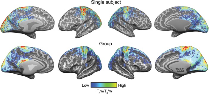
Single-subject (S6) and group (N = 6) (after cortex-based alignment) intracortical (myelin-related) maps. Anatomical contrast is projected on the individual reconstructed surfaces of both hemispheres (top row) and on the average (after cortex-based alignment) cortical surfaces (bottom row).
Analyzing the Intracortical Anatomical Contrast in the Temporal Lobe
In the temporal lobe, we observed a region of higher T1w/T2*w contrast in the vicinity of HG (see Supplementary Material for a description of the procedure used to create individual regions based on the average T1w/T2*w contrast). In each subject, the medial half of the HG was included (see Figs 3 and 4 for results of all single subjects). Most subjects displayed either a partial (see S2 in Fig. 3) or complete duplication of HG (right hemisphere in S6, Fig. 4), and in these subjects the densely myelin-related region extended to the regions in sulcus intermediate (SI; in case of an incomplete duplication), or onto Heschl's sulcus (HS) and the medial extent of the second HG (in case of a complete duplication). In one subject, also parts of PT were included in the region with the highest anatomical contrast related to myelin (right hemisphere of S1 in Fig. 3). Group maps replicated the pattern observed in single subjects, and previous reports on cortical myelination in auditory cortex at the group and single-subject level (Dick et al. 2012), with the strongest T1w/T2*w contrast in the medial portion of HG (Fig. 2).
Figure 3.

Single-subject (S1, S2, and S3) intracortical (myelin related) and tonotopic maps as obtained in experiment 1 (“tones”). Anatomical contrast and tonotopic maps are projected on the individual reconstructed surfaces of both hemispheres. Macroanatomical features (HG) and the highly myelinated region in the auditory cortex are outlined on all maps (solid black and dotted white line, respectively). The cluster resulting in the highest myelin-related content throughout the cortical depth is outlined in red.
Figure 4.

Single-subject (S4, S5, and S6) intracortical (b) (myelin-related), tonotopic (c and e), and tuning width (e) maps as obtained in session 1 (“tones”; c) and session 2 (“natural sounds”; d and e). Anatomical contrast and functional maps are projected on the individual reconstructed surfaces of both hemispheres. Macroanatomical features (HG) and the highly myelinated region in the auditory cortex are outlined on all maps (solid black and dotted white line, respectively). The cluster resulting in the highest myelin-related content throughout the cortical depth is outlined in red and is reported in (a).
After the parcellation procedure, we observed in all subjects a cluster coinciding with the region exhibiting the highest T1w/T2*w contrast averaged throughout the cortical depth (red lines in Figs 3 and 4). This cluster was characterized by the highest T1w/T2*w throughout the cortical depth consistently across all subjects (red cluster in Fig. 5; group cortical depth-dependent profiles). Its mean (across subjects) cortical thickness was 2.3 mm (0.1 mm standard deviation) in the left hemisphere and 2.2 mm (0.1 mm standard deviation) in the right hemisphere, in agreement with previous reports (Meyer et al. 2014). Three additional clusters were present in all subjects and hemispheres. One cluster occupied locations immediately bordering the first cluster, on medial HG/HS, lateral HG/HS, and anterior PT (green cluster in Fig. 5). This cluster showed a high T1w/T2*w signal close to the white matter, yet very weak T1w/T2*w signal at the cerebrospinal fluid boundary. A second cluster (shown in dark blue in Fig. 5) occupied medial HG/HS regions bilaterally. Additionally, the cluster included regions on PT and posterior STG in the left hemisphere. The T1w/T2*w signal of this third cluster was weaker than that of the first 2 clusters. The last cluster (shown in light blue in Fig. 5) showed the lowest T1w/T2*w signal throughout the cortical depth and occupied anterior locations. Specifically, regions on first transverse sulcus (FTS) adjacent to the insular cortex more medially on the right hemisphere compared with the left hemisphere, and anterior/middle STG in the left hemisphere, were included in this cluster. All cluster maps in Figure 5 are thresholded in order to show those regions that were consistently assigned to the same cluster in at least 4 of the 6 subjects (see Supplementary Fig. 2 for visualization of the consistency across subjects). We compared these clusters to previous postmortem reports of depth-dependent myelin content (Nieuwenhuys 2013). To do so, the depth-dependent myelin drawings of the regions in the temporal lobe (Nieuwenhuys 2013) were digitally acquired and the gray-scale values ([0–255]) were resampled in order to display myelin content at relative cortical depths (10–90% of cortical depth; see the bottom panel of Fig. 5).
Figure 5.

Cortex-based realigned group clusters (top) as identified by the parcellation procedure (k-means clustering). Individual maps are thresholded in order to show only vertices consistently assigned to the same cluster in at least 4 of the 6 subjects. Cortical depth-dependent profiles (middle) of anatomical contrast related to the centroid of each cluster (standard error computed across subjects) are reported together with the anatomical maps and color-coded accordingly. The bottom panel represents the cortical depth profiles for the regions ttr, tpartr, and tpari as digitized from Nieuwenhuys (2013).
The clustering results were also compared with an anatomical parcellation of the medial and lateral portion of the anterior HG (Supplementary Fig. 3). In agreement with the clustering approach, the depth-dependent profile of T1w/T2*w contrast was highest in the medial portion of HG. The anatomical parcellation showed increased variability across subjects especially for the lateral region in HG, indicating that the anatomical definition is not homogeneous (across subjects) in terms of the depth-dependent T1w/T2*w contrast.
Cortical Topographic Maps
We recorded functional responses while subjects listened to tones and natural sounds. In both cases, we observed consistent activation in the auditory cortex, including the Heschl's region (auditory core) (Formisano et al. 2003), and surrounding regions on PT and the STG (posterior and anterior). In both sessions and in each single hemisphere, the spatial distribution of best-frequency responses showed a large low-frequency region in the vicinity of HG. This low-frequency region was bordered anteriorly (on the FTS and on PP) and posteriorly (on HS and anterior PT) by regions preferring higher frequencies (see Figs 3 and 4 for all single-subject results). On the medial extremity of HG, often an additional region preferring low frequencies could be discriminated (see, e.g., left hemisphere of S2 in Fig. 3). Beyond the Heschl's regions, additional regions preferring low and high frequencies were present.
The estimation of spectral response profiles in session 2 allowed, in addition, the estimation of the voxels' tuning width. Tuning width reflects the frequency selectivity of a voxel, showing the range of frequencies around its main tonotopic peak to which a voxel displays sensitivity (Moerel et al. 2012). We observed a region of narrow tuning (see Fig. 4 for all single-subject results) along HG in each hemisphere, surrounded by regions of broader tuning. On PT, STG, and the superior temporal sulcus, additional regions of both broad and narrow tuning could be discriminated.
Relating Myelin-Based Contrast and Functional Properties in Individual Subjects
In order to compare anatomical and functional measures in the auditory cortex, we superimposed individual myelin-related maps and maps of tonotopy and tuning width. The selection of the region with the highest T1w/T2*w contrast (both in terms of its average content and its cortical depth profile) consistently highlighted a single tonotopic gradient for each single subject and hemisphere (Figs 3 and 4). In the individual subjects (hemispheres), the orientation of the high-to-low-frequency gradient in the selected region with the highest anatomical contrast related to myelin was variable. This observed variability may be due to macro-anatomical differences across subjects and their relation to functional variability (Da Costa et al. 2011). For a subset of subjects and hemispheres, also part of the additional low-frequency region at the most medial extremity of HG was included in the region of highest T1w/T2*w signal related to myelin (see, e.g., the right hemisphere of S2 in Fig. 3, and the left hemisphere of S5 in Fig. 4).
Finally, we investigated the tuning width properties of cortical regions with high anatomical myelin-related contrast. To this end, we analyzed the tuning width distribution of the cluster exhibiting the highest T1w/T2*w contrast and compared it with the distribution obtained over the whole auditory cortex. Figure 6 shows the histograms obtained for each hemisphere and subject (black lines, all auditory cortex; gray lines, selected regions based on T1w/T2*w contrast), displaying a relatively narrower tuning width in high T1w/T2*w contrast regions.
Figure 6.

Distribution of tuning width values within the auditory cortex (black line) and the region with the highest T1w/T2*w signal (gray line) for each individual subject and hemisphere. Vertical dotted lines represent the median of the distribution. The shift of tuning width toward narrow values (high values of tuning width) can be noted in each individual hemisphere.
Discussion
We investigated intracortical T1w/T2*w contrast of the human auditory cortex and its relationship to functional properties. Compared with previous in vivo investigations of combined anatomical–functional characteristics of the auditory core (Dick et al. 2012), here we take advantage of the higher temporal efficiency of the proposed procedure to acquire both anatomical and functional images in the same session. Furthermore, we exploit the higher resolution, specificity, and sensitivity of functional responses at high fields (Yacoub et al. 2001; Ugurbil et al. 2003) and validate the in vivo T1w/T2*w maps with both tonotopic (Formisano et al. 2003) and tuning width maps (Moerel et al. 2012).
In combination with cortical segmentation and advanced tools developed to define multiple surfaces at relative cortical depths, the high-resolution T1w/T2*w data allowed for a depth-dependent evaluation of myelin-related contrast within gray matter. Compared with previous in vivo studies of combined myeloarchitecture and function (Dick et al. 2012; Sereno et al. 2013), we also implemented a clustering procedure that allowed us to parcellate cortical regions based on T1w/T2*w depth-dependent profiles.
In individual subjects, we observe a region with high contrast in the medial portion of HG that contains a complete and narrowly tuned tonotopic gradient, which we interpret as primary auditory field human A1.
Benefits of 7T for the In Vivo Characterization of Myeloarchitecture
Mapping myeloarchitecture in vivo has recently received considerable attention (Geyer et al. 2011; Glasser and Van Essen 2011; Bock et al. 2013; Cohen-Adad et al. 2012; Dick et al. 2012; Sereno et al. 2013; Cohen-Adad 2013; Glasser et al. 2013). At conventional magnetic field strength (up to 3T), in vivo myeloarchitectonic mapping in humans has been pursued with quantitative techniques (such as T1 mapping) (Sigalovsky et al. 2006; Barazany and Assaf 2011; Sereno et al. 2013), standard anatomical imaging (Barbier et al. 2002; Walters et al. 2003), and optimized acquisitions of 1 or 2 images per subject (Glasser and Van Essen 2011; Bock et al. 2013). While these investigations showed the potential benefits of acquiring images whose contrast highlights intracortical differences, the need for high-resolution images for a precise definition of areas (Geyer et al. 2011) resulted in temporally inefficient protocols and/or reduced volume coverage. As a result, when combining myeloarchitectonic and functional measures, separate sessions at different field strengths have been used (Dick et al. 2012; Sereno et al. 2013). Compared with these studies, we acquire both anatomical and functional data in the same session and measure functional responses at higher resolution and functional specificity.
In 25 min, we obtained whole-brain high-resolution (0.6 mm isotropic) images at high fields with: gray/white matter contrast, vascular information, and T1w/T2*w contrast, leaving time for functional imaging within the same session.
Parcellating Human Auditory Cortex
To investigate the benefit of measuring anatomical contrast related to myelin in vivo, we applied our new technique to the problem of localizing auditory cortical areas in humans, an issue that could not yet be resolved from imaging macroanatomical features (Penhune et al. 1996) or tonotopic mapping alone (Humphries et al. 2010; Striem-Amit et al. 2011; Langers and van Dijk 2012; Moerel et al. 2012).
Maps of T1w/T2*w outlined a region including the most medial section of HG contrast was highest (see, e.g., Figs 3 and 4). This result is consistent with previous in vivo myeloarchitectural imaging results (Sigalovsky et al. 2006; Geyer et al. 2011; Cohen-Adad et al. 2012; Dick et al. 2012). Furthermore, it is in agreement with postmortem staining studies in monkeys and humans, which revealed that primary auditory regions (i.e., core) are more densely myelinated than the surround, with the core being divided in a more myelinated portion caudally and a less myelinated portion rostrally (Hackett et al. 1998; Hackett et al. 2001). Beyond this overall difference in myelin content, early reports indicated that primary auditory regions are unistriate with a heavily myelinated middle cortical layer (i.e., region temporalis transversa [ttr] as defined by (Hopf 1954) and reported more recently in Nieuwenhuys (2013)). However, a more recent study of auditory cortex myeloarchitecture showed the auditory core to be divided in a medial astriate section and lateral unistriate section (Hackett et al. 2001). Possibly because of insufficient resolution/sensitivity, our cortical depth-dependent analysis did not show evidence of a heavily myelinated middle cortical layer (i.e., stria) in the most medial section of HG. However, this region of the temporal lobe exhibited the highest contrast throughout the whole cortical depth and decreasing toward the surface (Fig. 5). The highest T1w/T2*w signal at all cortical depths in comparison with other regions in the temporal lobe suggests that this region may be equivalent to the most medial portion of ttr (Nieuwenhuys 2013; see the lower portion of Fig. 5 for a digital representation of ttr). Our combined anatomical and functional analyses showed that this region on medial HG consistently coincided with a single high-to-low tonotopic gradient in each individual subject (Figs 3 and 4). This observation was replicated in tonotopy maps computed on natural sounds, where we additionally revealed that the same region showed narrow tuning properties (Figs 4 and 6). In the monkey, a narrowly tuned primary auditory cortex contains 2 tonotopic gradients that define fields A1 and R (Hackett et al. 1998; Rauschecker and Tian 2004). Consequently, the combination of anatomical and functional data identified the cluster with the highest T1w/T2*w contrast in the medial portion of HG as the human homolog of monkey primary field A1 (hA1; Hackett et al. 2001). This result represents a difference with a previous study (Dick et al. 2012), which suggested that the densely myelinated region in the medial portion of HG (identified by correspondence to a probabilistic atlas of “cyto-architecture”) corresponds with the entire auditory core (thus the union of A1 and R) and shows a “plateau” of the intracortical contrast in correspondence of middle cortical depths (Dick et al. 2012). Our results, however, were obtained with a different methodology, which involved non-quantitative (vs. quantitative) anatomical mapping optimized for time efficiency, a higher magnetic field strength for the acquisition of both anatomical (7T vs. 3T) and functional (7T vs. 1.5T) data, and a data-driven clustering approach based on single-subject data rather than probabilistically pre-specified anatomical regions. Further investigations will be needed to understand the nature of this difference in results across studies and with respect to postmortem investigations.
The cortical depth-dependent analysis also allowed the identification of 3 additional clusters with consistent depth-dependent profiles, but lower spatial consistency across subjects. The first encompassed medial HG/HS, lateral HG/HS, and anterior PT (green cluster in Fig. 5). When comparing its cortical depth-dependent T1w/T2*w contrast to the primary cluster (red in Fig. 5), significant differences can be noted especially in middle to superficial portion of the cortex. Because of its anatomical location, this cluster may resemble the human homolog of area R. The second cluster extends medially in HG/HS bilaterally and including regions on PT and posterior STG (blue cluster in Fig. 5) and is characterized by a T1w/T2*w contrast, which is overall lower than the primary cluster, with the biggest difference in both deep and middle gray matter. Its anatomical location and gradually decreasing T1w/T2*w contrast suggest a possible correspondence to parts of the region temporalis para transversa (tpartr) (Nieuwenhuys 2013; see the lower portion of Fig. 5 for a digital representation of tpartr). Finally, the cluster exhibiting the overall lowest T1w/T2*w signal (especially in deep and middle gray matter) and including regions adjacent to the insular cortex bilaterally (light blue cluster in Fig. 5) may coincide with parts of the regio temporalis para insularis (tpari; Nieuwenhuys 2013; see the lower portion of Fig. 5 for a digital representation of tpari). A previous in vivo study of auditory cortical myeloarchitecture in vivo (Dick et al. 2012) highlighted a significant difference in myelin content between core and lateral belt regions mostly in middle layers between portions of HG. For the 3 non-primary clusters reported here, significant differences in anatomical contrast with respect to the primary cluster were confined to either the deep and middle layers (blue and cyan clusters) or an increasing difference moving toward the cortical surface (green cluster). None of our clusters can be associated with specific portions of belt as previously identified in Hackett et al. (2001). The suggested correspondence to the regions, as defined by Hopf (1954) and reported in Nieuwenhuys (2013) (Fig. 5), is based on the difference in myelin content throughout the cortical depths and anatomical locations. Future histological validations and functional investigations are needed to assess the relevance of these clusters and their intersubject variability.
Limitations and Future Studies
While the method proposed here allows the time-efficient acquisition of intracortical contrast maps, a few limitation of this method must be noted. First, despite the increased time efficiency of our scans, significant subject motion during the data acquisition may affect data quality, as it is visible in some of our acquisitions (see sagittal cuts through the visual cortex of subjects 1 and 4 in Supplementary Fig. 1). In future studies, this effect may be minimized by using methods of prospective motion correction (Maclaren et al. 2013). Secondly, the proposed contrast weighted acquisition techniques necessitate more advanced postprocessing strategies to deal with residual low-frequency biases in the anatomical data compared with quantitative approaches (Sigalovsky et al. 2006; Fukunaga et al. 2010; Barazany and Assaf 2011; Geyer et al. 2011; Cohen-Adad et al. 2012; Dick et al. 2012; Sereno et al. 2013). Thirdly, the shorter acquisition time dedicated to anatomical scans may result in a lower signal-to-noise ratio. Compared with previous high field investigations with comparable spatial resolution but longer time scans (i.e., 60 min; Geyer et al. 2011), myeloarchitectonic features such as the stria of gennari in visual cortex were not unambiguously identified in all subjects in our data (Supplementary Fig. 1). Finally, our results may be affected by the magnetic field orientation-dependent contrast of the T2*-weighted images (Cohen-Adad et al. 2012).
In spite of these limitations, the whole-brain pattern of T1w/T2*w contrast reported here is similar to previously published results at both low and high fields (Geyer et al. 2011; Bock et al. 2012; Cohen-Adad et al. 2012; Sereno et al. 2013), with high contrast evident in primary sensory areas (visual, motor, and auditory; see Fig. 2 for group results). While these results suggest that the source of the T1w/T2*w contrast is similar in nature to the one targeted in previous studies, with both iron and myelin being influential to the generation of the variations shown here, further quantitative analyses will be needed to understand the differences between all acquisition schemes.
Supplementary Material
Supplementary material can be found at: http://www.cercor.oxfordjournals.org/.
Funding
This work was supported in part by the National Institute of Health (NIH) Human Connectome Project (NIH U54MH091657), the National Institute of Neurological Disorders and Stroke (NINDS; P30 NS076408), Biomedical Technology Resource Centers (BTRC) National Center for Research Resources (NCRR; P41 RR08079), the National Institute of Biomedical Imaging and Bioengineering (NIBIB; P41 EB015894), the W.M. Keck Foundation, and MIND institute. The 7T magnet purchase was funded in part by National Science Foundation (DBI-9907842) and the National Institute of Health (S10 RR1395). E.F. was funded by NWO VICI (grant 453-12-002). F.D.M. was funded by NWO VIDI (grant 864-13-012).
Supplementary Material
Notes
Conflict of Interest: The authors have no conflict of interest to declare.
References
- Abosch A, Yacoub E, Ugurbil K, Harel N. 2010. An assessment of current brain targets for deep brain stimulation surgery with susceptibility-weighted imaging at 7 tesla. Neurosurgery. 67:1745–1756; discussion 1756. [DOI] [PMC free article] [PubMed] [Google Scholar]
- Barazany D, Assaf Y. 2011. Visualization of cortical lamination patterns with magnetic resonance imaging. Cereb Cortex. 22:2016–2023. [DOI] [PubMed] [Google Scholar]
- Barbier EL, Marrett S, Danek A, Vortmeyer A, van Gelderen P, Duyn J, Bandettini P, Grafman J, Koretsky AP. 2002. Imaging cortical anatomy by high-resolution MR at 3.0T: detection of the stripe of Gennari in visual area 17. Magn Reson Med. 48:735–738. [DOI] [PubMed] [Google Scholar]
- Bock NA, Hashim E, Janik R, Konyer NB, Weiss M, Stanisz GJ, Turner R, Geyer S. 2013. Optimizing T(1)-weighted imaging of cortical myelin content at 3.0T. NeuroImage. 65:1–12. [DOI] [PubMed] [Google Scholar]
- Bock NA, Hashim E, Kocharyan A, Silva AC. 2011. Visualizing myeloarchitecture with magnetic resonance imaging in primates. Ann N Y Acad Sci. 1225(Suppl 1):E171–E181. [DOI] [PMC free article] [PubMed] [Google Scholar]
- Bock NA, Kocharyan A, Liu JV, Silva AC. 2009. Visualizing the entire cortical myelination pattern in marmosets with magnetic resonance imaging. J Neurosci Methods. 185:15–22. [DOI] [PMC free article] [PubMed] [Google Scholar]
- Carmichael DW, Thomas DL, De Vita E, Fernandez-Seara MA, Chhina N, Cooper M, Sunderland C, Randell C, Turner R, Ordidge RJ. 2006. Improving whole brain structural MRI at 4.7 Tesla using 4 irregularly shaped receiver coils. NeuroImage. 32:1176–1184. [DOI] [PubMed] [Google Scholar]
- Celesia GG. 1976. Organization of auditory cortical areas in man. Brain. 99:403–414. [DOI] [PubMed] [Google Scholar]
- Clare S, Bridge H. 2005. Methodological issues relating to in vivo cortical myelography using MRI. Hum Brain Mapp. 26:240–250. [DOI] [PMC free article] [PubMed] [Google Scholar]
- Clark VP, Courchesne E, Grafe M. 1992. In vivo myeloarchitectonic analysis of human striate and extrastriate cortex using magnetic resonance imaging. Cereb Cortex. 2:417–424. [DOI] [PubMed] [Google Scholar]
- Cohen-Adad J. 2013. What can we learn from T* maps of the cortex? NeuroImage. doi:10.1016/j.neuroimage.2013.01.023. [DOI] [PubMed]
- Cohen-Adad J, Polimeni JR, Helmer KG, Benner T, McNab JA, Wald LL, Rosen BR, Mainero C. 2012. T(2)* mapping and B(0) orientation-dependence at 7T reveal cyto- and myeloarchitecture organization of the human cortex. NeuroImage. 60:1006–1014. [DOI] [PMC free article] [PubMed] [Google Scholar]
- Da Costa S, van der Zwaag W, Marques JP, Frackowiak RSJ, Clarke S, Saenz M. 2011. Human primary auditory cortex follows the shape of Heschl's gyrus. J Neurosci. 31:14067–14075. [DOI] [PMC free article] [PubMed] [Google Scholar]
- De Martino F, Moerel M, van de Moortele PF, Ugurbil K, Goebel R, Yacoub E, Formisano E. 2013. Spatial organization of frequency preference and selectivity in the human inferior colliculus. Nat Commun. 4:1386. [DOI] [PMC free article] [PubMed] [Google Scholar]
- Dick F, Tierney AT, Lutti A, Josephs O, Sereno M, Weiskopf N. 2012. In Vivo functional and myeloarchitectonic mapping of human primary auditory areas. J Neurosci. 32:16095–16105. [DOI] [PMC free article] [PubMed] [Google Scholar]
- Duyn JH, van Gelderen P, Li T-Q, de Zwart JA, Koretsky AP, Fukunaga M. 2007. High-field MRI of brain cortical substructure based on signal phase. Proc Natl Acad USA. 104:11796–11801. [DOI] [PMC free article] [PubMed] [Google Scholar]
- Edmister WB, Talavage TM, Ledden PJ, Weisskoff RM. 1999. Improved auditory cortex imaging using clustered volume acquisitions. Hum Brain Mapp. 7:89–97. [DOI] [PMC free article] [PubMed] [Google Scholar]
- Feinberg DA, Hale JD, Watts JC, Kaufman L, Mark A. 1986. Halving MR imaging time by conjugation: demonstration at 3.5 kG. Radiology. 161:527–531. [DOI] [PubMed] [Google Scholar]
- Formisano E, Kim DS, Di Salle F, van De Moortele P-F, Ugurbil K, Goebel R. 2003. Mirror-symmetric tonotopic maps in human primary auditory cortex. Neuron. 40:859–869. [DOI] [PubMed] [Google Scholar]
- Fukunaga M, Li T-Q, van Gelderen P, de Zwart JA, Shmueli K, Yao B, Lee J, Maric D, Aronova MA, Zhang G, et al. 2010. Layer-specific variation of iron content in cerebral cortex as a source of MRI contrast. Proc Natl Acad Sci USA. 107:3834–3839. [DOI] [PMC free article] [PubMed] [Google Scholar]
- Galaburda A, Sanides F. 1980. Cytoarchitectonic organization of the human auditory cortex. J Comp Neurol. 190:597–610. [DOI] [PubMed] [Google Scholar]
- Garwood M, Ugurbil K. 1992. B1 insensitive adiabatic RF pulses In: Rudin M, editor. In vivo magnetic resonance spectroscopy I: probeheads and radiofrequency pulses spectrum analysis, NMR basic principles and progress, Vol. 26. Berlin: Springer-Verlag.
- Geyer S, Weiss M, Reimann K, Lohmann G, Turner R. 2011. Microstructural parcellation of the human cerebral cortex—from Brodmann's post-mortem map to in vivo mapping with high-field magnetic resonance imaging. Front Hum Neurosci. 5:19. [DOI] [PMC free article] [PubMed] [Google Scholar]
- Glasser MF, Goyal MS, Preuss TM, Raichle ME, Van Essen DC. 2013. Trends and properties of human cerebral cortex: correlations with cortical myelin content. NeuroImage. doi:10.1016/j.neuroimage.2013.03.060. [DOI] [PMC free article] [PubMed]
- Glasser MF, Van Essen DC. 2011. Mapping human cortical areas in vivo based on myelin content as revealed by T1- and T2-weighted MRI. J Neurosci. 31:11597–11616. [DOI] [PMC free article] [PubMed] [Google Scholar]
- Goebel R, Esposito F, Formisano E. 2006. Analysis of functional image analysis contest (FIAC) data with brainvoyager QX: from single-subject to cortically aligned group general linear model analysis and self-organizing group independent component analysis. Hum Brain Mapp. 27:392–401. [DOI] [PMC free article] [PubMed] [Google Scholar]
- Griswold MA, Jakob PM, Heidemann RM, Nittka M, Jellus V, Wang J, Kiefer B, Haase A. 2002. Generalized autocalibrating partially parallel acquisitions (GRAPPA). Magn Reson Med. 47:1202–1210. [DOI] [PubMed] [Google Scholar]
- Hackett TA, Preuss TM, Kaas JH. 2001. Architectonic identification of the core region in auditory cortex of macaques, chimpanzees, and humans. J Comp Neurol. 441:197–222. [DOI] [PubMed] [Google Scholar]
- Hackett TA, Stepniewska I, Kaas JH. 1998. Subdivisions of auditory cortex and ipsilateral cortical connections of the parabelt auditory cortex in macaque monkeys. J Comp Neurol. 394:475–495. [DOI] [PubMed] [Google Scholar]
- Hinds O, Polimeni JR, Rajendran N, Balasubramanian M, Wald LL, Augustinack JC, Wiggins G, Rosas HD, Fischl B, Schwartz EL. 2008. The intrinsic shape of human and macaque primary visual cortex. Cereb Cortex. 18:2586–2595. [DOI] [PMC free article] [PubMed] [Google Scholar]
- Hopf A. 1954. Die myeloarchitektonik des isocortex temporalis beim menschen. J Hirnforsch. 1:443–496. [Google Scholar]
- Humphries C, Liebenthal E, Binder JR. 2010. Tonotopic organization of human auditory cortex. NeuroImage. 50:1202–1211. [DOI] [PMC free article] [PubMed] [Google Scholar]
- Jones SE, Buchbinder BR, Aharon I. 2000. Three-dimensional mapping of cortical thickness using Laplace's equation. Hum Brain Mapp. 11:12–32. [DOI] [PMC free article] [PubMed] [Google Scholar]
- Khan R, Zhang Q, Darayan S, Dhandapani S, Katyal S, Greene C, Bajaj C, Ress D. 2011. Surface-based analysis methods for high-resolution functional magnetic resonance imaging. Graph Models. 73:313–322. [DOI] [PMC free article] [PubMed] [Google Scholar]
- Langers DR, van Dijk P. 2012. Mapping the tonotopic organization in human auditory cortex with minimally salient acoustic stimulation. Cereb Cortex. 22:2024–2038. [DOI] [PMC free article] [PubMed] [Google Scholar]
- Maclaren J, Herbst M, Speck O, Zaitsev M. 2013. Prospective motion correction in brain imaging: a review. Magn Reson Med. 69:621–636. [DOI] [PubMed] [Google Scholar]
- Meyer M, Liem F, Hirsiger S, Jancke L, Hanggi J. 2014. Cortical surface area and cortical thickness demonstrate differential structural asymmetry in auditory-related areas of the human cortex. Cereb Cortex. 24:2541–2552. [DOI] [PubMed] [Google Scholar]
- Moerel M, De Martino F, Formisano E. 2012. Processing of natural sounds in human auditory cortex: tonotopy, spectral tuning and relation to voice-sensitivity. J Neurosci. 32:14205–14216. [DOI] [PMC free article] [PubMed] [Google Scholar]
- Morosan P, Rademacher J, Schleicher A, Amunts K, Schormann T, Zilles K. 2001. Human primary auditory cortex: cytoarchitectonic subdivisions and mapping into a spatial reference system. NeuroImage. 13:684–701. [DOI] [PubMed] [Google Scholar]
- Nieuwenhuys R. 2013. The myeloarchitectonic studies on the human cerebral cortex of the Vogt-Vogt school, and their significance for the interpretation of functional neuroimaging data. Brain Struct Funct. 218:303–352. [DOI] [PubMed] [Google Scholar]
- Penhune VB, Zatorre RJ, MacDonald JD, Evans AC. 1996. Interhemispheric anatomical differences in human primary auditory cortex: probabilistic mapping and volume measurement from magnetic resonance scans. Cereb Cortex. 6:661–672. [DOI] [PubMed] [Google Scholar]
- Polimeni JR, Fischl B, Greve DN, Wald LL. 2010. Laminar analysis of 7T BOLD using an imposed spatial activation pattern in human V1. NeuroImage. 52:1334–1346. [DOI] [PMC free article] [PubMed] [Google Scholar]
- Rademacher J, Morosan P, Schormann T, Schleicher A, Werner C, Freund HJ, Zilles K. 2001. Probabilistic mapping and volume measurement of human primary auditory cortex. NeuroImage. 13:669–683. [DOI] [PubMed] [Google Scholar]
- Rauschecker J, Tian B. 2004. Processing of band-passed noise in the lateral auditory belt cortex of the rhesus monkey. J Neurophysiol. 91:2578. [DOI] [PubMed] [Google Scholar]
- Rivier F, Clarke S. 1997. Cytochrome oxidase, acetylcholinesterase, and NADPH-diaphorase staining in human supratemporal and insular cortex: evidence for multiple auditory areas. NeuroImage. 6:288–304. [DOI] [PubMed] [Google Scholar]
- Sanchez-Panchuelo RM, Francis ST, Schluppeck D, Bowtell RW. 2012. Correspondence of human visual areas identified using functional and anatomical MRI in vivo at 7T. J Magn Reson Imaging. 35:287–299. [DOI] [PubMed] [Google Scholar]
- Sereno MI, Lutti A, Weiskopf N, Dick F. 2013. Mapping the human cortical surface by combining quantitative T1 with retinotopy. Cereb Cortex. 23:2261–2268. [DOI] [PMC free article] [PubMed] [Google Scholar]
- Sigalovsky IS, Fischl B, Melcher JR. 2006. Mapping an intrinsic MR property of gray matter in auditory cortex of living humans: a possible marker for primary cortex and hemispheric differences. NeuroImage. 32:1524–1537. [DOI] [PMC free article] [PubMed] [Google Scholar]
- Striem-Amit E, Hertz U, Amedi A. 2011. Extensive cochleotopic mapping of human auditory cortical fields obtained with phase-encoding fMRI. PLoS ONE. 6:e17832. [DOI] [PMC free article] [PubMed] [Google Scholar]
- Talavage TM, Hall DA. 2012. How challenges in auditory fMRI led to general advancements for the field. NeuroImage. 62:641–647. [DOI] [PMC free article] [PubMed] [Google Scholar]
- Trampel R, Ott DV, Turner R. 2011. Do the congenitally blind have a stria of Gennari? First intracortical insights in vivo. Cereb Cortex. 21:2075–2081. [DOI] [PubMed] [Google Scholar]
- Ugurbil K, Adriany G, Andersen P, Chen W, Garwood M, Gruetter R, Henry P-G, Kim S-G, Lieu H, Tkac I, et al. 2003. Ultrahigh field magnetic resonance imaging and spectroscopy. Magn Reson Imaging. 21:1263–1281. [DOI] [PubMed] [Google Scholar]
- van de Moortele P-F, Auerbach EJ, Olman C, Yacoub E, Ugurbil K, Moeller S. 2009. T1 weighted brain images at 7 Tesla unbiased for Proton Density, T2* contrast and RF coil receive B1 sensitivity with simultaneous vessel visualization. NeuroImage. 46:432–446. [DOI] [PMC free article] [PubMed] [Google Scholar]
- Waehnert MD, Dinse J, Weiss M, Streicher MN, Waehnert P, Geyer S, Turner R, Bazin PL. 2014. Anatomically motivated modeling of cortical laminae. NeuroImage. 93(Pt 2):210–220. [DOI] [PubMed] [Google Scholar]
- Walters NB, Egan GF, Kril JJ, Kean M, Waley P, Jenkinson M, Watson JD. 2003. In vivo identification of human cortical areas using high-resolution MRI: an approach to cerebral structure-function correlation. Proc Natl Acad Sci USA. 100:2981–2986. [DOI] [PMC free article] [PubMed] [Google Scholar]
- Yacoub E, Shmuel A, Pfeuffer J, van De Moortele P-F, Adriany G, Andersen P, Vaughan JT, Merkle H, Ugurbil K, Hu X. 2001. Imaging brain function in humans at 7 Tesla. Magn Reson Med. 45:588–594. [DOI] [PubMed] [Google Scholar]
- Yoshiura T, Higano S, Rubio A, Shrier DA, Kwok WE, Iwanaga S, Numaguchi Y. 2000. Heschl and superior temporal gyri: low signal intensity of the cortex on T2-weighted MR images of the normal brain. Radiology. 214:217–221. [DOI] [PubMed] [Google Scholar]
- Zilles K, Amunts K. 2012. Architecture of the cerebral cortex. In: Mai J, Paxinos G, editors. The human nervous system, 3rd ed San Diego (USA): Elsevier Academic Press. [Google Scholar]
- Zwanenburg JJ, Versluis MJ, Luijten PR, Petridou N. 2011. Fast high resolution whole brain T2* weighted imaging using echo planar imaging at 7T. NeuroImage. 56:1902–1907. [DOI] [PubMed] [Google Scholar]
Associated Data
This section collects any data citations, data availability statements, or supplementary materials included in this article.