Functional Clusters, Hubs, and Communities in the Cortical Microconnectome

Abstract

Although relationships between networks of different scales have been observed in macroscopic brain studies, relationships between structures of different scales in networks of neurons are unknown. To address this, we recorded from up to 500 neurons simultaneously from slice cultures of rodent somatosensory cortex. We then measured directed effective networks with transfer entropy, previously validated in simulated cortical networks. These effective networks enabled us to evaluate distinctive nonrandom structures of connectivity at 2 different scales. We have 4 main findings. First, at the scale of 3–6 neurons (clusters), we found that high numbers of connections occurred significantly more often than expected by chance. Second, the distribution of the number of connections per neuron (degree distribution) had a long tail, indicating that the network contained distinctively high-degree neurons, or hubs. Third, at the scale of tens to hundreds of neurons, we typically found 2–3 significantly large communities. Finally, we demonstrated that communities were relatively more robust than clusters against shuffling of connections. We conclude the microconnectome of the cortex has specific organization at different scales, as revealed by differences in robustness. We suggest that this information will help us to understand how the microconnectome is robust against damage.

Introduction

Multiscale structure is a hallmark of many complex systems (Simon 1962; Bar-Yam 2004; Werner 2010) and has been suggested to confer adaptability (Simon 1962), robustness (Carlson and Doyle 2002), and ease of information exchange (Dodds et al. 2003). As the brain is perhaps the epitome of a complex system, one naturally would expect to find multiscale structure there (Leergaard et al. 2012). Indeed, functional magnetic resonance imaging (fMRI) data have provided evidence for multiscale (Bassett et al. 2006) and hierarchical (Meunier et al. 2009) functional networks in the human cortex. Furthermore, simultaneous evaluation or comparison of structures at multiple scales has also been attempted in macroscopic brain studies (Sporns et al. 2007; Bassett et al. 2011; Shen et al. 2012; Shimono 2013). Within a typical fMRI voxel, however, there are hundreds to thousands of neurons. It has remained an open question as to how structures at multiple scales relate to each other at this smaller level of neuronal networks.

Broadly speaking, functional connectivity can be either undirected or directed. Undirected functional connectivity is typically used to denote a correlation or co-activation between 2 nodes in a network (e.g., Biswal et al. 1995; Schneidman et al. 2006). Directed functional connectivity, sometimes called “effective” connectivity, denotes a temporal sequence of activation or a direction of causality between nodes (Friston 1994; Bonifazi et al. 2009; Takahashi et al. 2010). To determine effective connectivity among several hundred spiking cortical neurons, it is therefore necessary to record data simultaneously at millisecond temporal resolution to match the synaptic delays of 1–20 ms reported in cortex (Mason et al. 1991; Swadlow 1994). As we explain below, recent advances in multielectrode array technology have now made this possible (Litke et al. 2004; Field et al. 2010). We sought to apply this technology to answer 2 questions. First, are there structures at multiple scales (hubs, clusters, and communities) in the effective connectivity of hundreds of cortical neurons? Second, if structures at multiple scales exist, how do these structures relate to each other?

To pursue these questions, we used a 512-electrode array system to record spontaneous activity at 20 kHz sampling rate in 25 slice cultures of mouse somatosensory cortex. On average, we recorded 310 ± 127 [mean ± standard deviation (SD)] neurons from each culture for 1 h or more. Although many metrics of effective connectivity have been proposed (Aertsen et al. 1989; Garofalo et al. 2009; Pajevic and Plenz 2009; Friston 2011), we selected transfer entropy (TE; Schreiber 2000) because several studies found it to compare favorably in accuracy with other metrics (Lungarella et al. 2007; Garofalo et al. 2009; Ito et al. 2011; Stetter et al. 2012; Vincent et al. 2012; Orlandi et al. 2013).

With this metric, we sought to answer the questions above and to verify that our findings were robust with respect to possible errors in spike sorting, and to criteria for accepting an effective connection. Portions of this work have been previously presented in abstract form (Shimono and Beggs 2011a, 2011b, 2014).

Materials and Methods

Culture Preparation

All neural tissue from animals was prepared according to guidelines from the National Institutes of Health and all animal procedures were approved by the Animal Care and Use Committees at Indiana University and at the University of California, Santa Cruz, CA, USA. For these studies, we used organotypic cultures because they preserve many of the features characteristic of cortex, including neuronal morphology (Klostermann and Wahle 1999), cytoarchitecture (Caeser et al. 1989; Gotz, Bolz 1992), precise intracortical connectivity (Bolz et al. 1990), and intrinsic electrophysiological properties (Plenz and Aertsen 1996). In addition, they produce a variety of emergent network activity patterns that have been found in vivo, including precisely timed responses (Buonomano 2003), UP states (Johnson, Buonomano 2007), oscillations (Baker et al. 2006; Gireesh and Plenz 2008), synchrony (Beggs and Plenz 2004; Baker et al. 2006), waves (Harris-White et al. 1998), repeating activity patterns (Beggs and Plenz 2004; Ikegaya et al. 2004), and neuronal avalanches (Beggs and Plenz 2003; Friedman et al. 2012).

When cortical slice cultures are grown with subcortical target structures, as done here, it has been shown that they form appropriate connections that are not exuberant (Leiman and Seil 1986; Baker and van Pelt 1997). We prepared organotypic cultures using methods previously reported (Tang et al. 2008). Briefly, brains from postnatal day 6 (P6) to P7 black 6 mouse pups (Harlan, RRID:Charles_River:24101632) were removed under a sterile hood and placed in chilled Gey's balanced salt solution (Sigma) for 1 h at 0 °C. After 30 min, half the solution was changed. Brains were next blocked into 5-mm³ sections containing somatosensory cortex (Paxinos and Watson 2007). Blocks were then sliced with a thickness of 400 μm.

Each slice was placed on a small circular cutout of permeable membrane (Millipore, Billerica, MA, USA) that was then placed on top of a larger membrane that spanned a culture well. Culture medium consisted of Hank's balanced salt solution (Sigma; H9394) 1:4, Minimum essential medium (Sigma; M4083) 2:4, horse serum (Sigma; H1270) 1:4, and 4 mL l-glutamine, with penicillin/streptomycin 1:1000 volume of media (Sigma; P4083). Slices were maintained at an interface between medium below and atmosphere above.

The plates of wells were incubated at 37 °C in humidified atmosphere with 5% CO₂.

Recording and Spike Sorting

After 2–3 weeks, the cultures were then gently placed on a microelectrode recording array by lifting the small circular cutout of membrane with tweezers. Each culture was placed tissue side down, with the membrane facing up. We attempted to place the tissue such that somatosensory cortex was on the electrode array (Fig. 1a). During recording, cultures were perfused at 1 mL/min with culture medium that was saturated with 95% O₂/5% CO₂. The perfusate was thermostatically kept at 37 °C. Spontaneous activity was recorded for 1.5 h. The first 0.5 h was not used in analysis. Spikes were recorded with a 512-electrode array system that has been used previously for retinal (Shlens et al. 2006; Field et al. 2010) and cortical (Tang et al. 2008; Friedman et al. 2012) experiments. The outline of the array was rectangular (1.8 mm × 0.9 mm) and electrodes were arranged in a hexagonal lattice with an interelectrode distance of 60 μm (Fig. 1b). Spike sorting was done offline as previously described (Litke et al. 2004; Tang et al. 2008). Briefly, signals that crossed a threshold of 8 SDs were marked, and the waveforms found on the marked electrode and its 6 adjacent neighbors were projected into 5D principal component space. A mixture of Gaussians model was fit to the distribution of features based on maximum likelihood. Only the neurons that had well-separated clusters in principal components space and had no refractory period violations were used in further analysis. The close 60-μm spacing between electrodes allows an action potential from one neuron to be detected by 7 electrodes with this 512 array. Because action potential amplitude falls off with distance, it is possible to use the unique combination of amplitudes from the 7 electrodes to triangulate the locations of the neurons (Litke et al. 2004).

Figure 1.

Experimental setup. (a) Micrograph of cortical slice culture on a 512-electrode array. Array is ∼1 × 2 mm, outlined for visibility. Small dots are electrodes, arranged hexagonally with 60 μm spacing. (b) Representative raster of activity. Dots represent spikes from 260 sorted neurons, shown for 300 s. (c) Schematic of transfer entropy (TE) showing 2 binned spike trains. TE evaluates how much neuron J's past spiking activity improves the prediction of neuron I's activity beyond the prediction based on neuron I's activity from the previous time bin. Here, delay indicates time lag chosen for the spiking activity of neuron J. (d) Definition of the Coincidence index (CI). When TE was plotted as a function of delay, CI was the ratio of area under the peak (A) to total area under the curve (A + B).

The quality of the data collected for this study had a unique combination of features that made it particularly useful for uncovering effective connectivity in neural networks at this scale. The high temporal resolution of the recordings allowed the sequence of spike activations to be identified in many cases, letting us measure directed, rather than undirected, connections. The close electrode spacing (∼60 μm) was within the radius of most synaptic contacts between cortical pyramidal neurons (Song et al. 2005), and enhanced the probability that recorded neurons would share direct synaptic contacts. The large number of neurons simultaneously recorded, as well as the long recording durations (1 h or more) enhanced statistical power, allowing many connections to be identified that would have otherwise gone undetected. Very few previous studies have been able to combine all of these features simultaneously.

Effective Connectivity Metric

There is a large and growing literature on metrics for effective connectivity (e.g., Hlavackova-Schindler et al. 2007); we selected TE because several previous studies (Lungarella et al. 2007; Garofalo et al. 2009; Ito et al. 2011; Stetter et al. 2012; Vincent et al. 2012), indicated that it compared quite favorably with other metrics in terms of accuracy. As an information-theoretic measure, TE is also capable of detecting nonlinear interactions between neurons (Schreiber 2000). More generally, TE is a directed (asymmetric), measure of influence that can be applied to 2 time series—here we used spike trains binned at a resolution of 1 ms. In neuroscience terms, TE is positive if including information about neuron J's spiking activity improves the prediction of neuron I's activity beyond the prediction based on neuron I's past alone (Fig. 1c). The original definition of TE (Schreiber 2000) was given as:

$$\text{T}{\text{E}}_{J\to I}=\sum p(i_{t+1},i_t^{(k)},j_t^{(l)}){\log }_2\frac{p(i_{t+1}|i_t^{(k)},j_t^{(l)})}{p(i_{t+1}|i_t^{(k)})}.$$ (1)

Here, i_t denoted the status of neuron I at time t, and could be either 1 or 0, indicating a spike or no spike, respectively; j_t denoted the status of neuron J at time t; i_t+1 denoted the status of neuron I at time t + 1; p denoted the probability of having the status in the following parentheses; and the vertical bar in the parentheses denoted the conditional probability. The sum was over all possible combinations of i_t+1, $i_t^{(k)}$, and $j_t^{(l)}$. The parameters k and l gave the order of TE, meaning the number of time bins in the past that were used to calculate the histories of systems I and J, respectively. Here, we used k = l = 1, so that only single time bins were considered. This was because the connectivity matrix produced from higher-order TE was very similar to that produced by first order TE (results for k = 3, l = 2 are shown in Supplementary Fig. 2c). Further comparisons were also essentially similar. We used logarithms with base 2 so that our units would be bits, although in some figures we used base 10 so as to cover a wider range of data. Given that synaptic delays between cortical neurons could span several milliseconds (Bartho et al. 2004; Sirota et al. 2008), we adopted a version of TE that allowed delays between neuron I and J. To continue to consider the system's own history, we kept a 1-bin delay for neuron I, assuming that neuron I depended mostly on its closest previous state. To account for synaptic delays between neurons, the time bin of neuron J was delayed by d bins, as described below. Taking these modifications into account, we used a delayed version of TE, given by:

$$\text{T}{\text{E}}_{J\to I}(d)=\sum p(i_t,i_{t-1},j_{t-d}){\log }_2\frac{p(i_t|i_{t-1},i_{t-d})}{p(i_t|i_{t-1})}.$$ (2)

Here other terms were as defined in Equation (1). When TE between 2 neurons was plotted as a function of different delays d, it often showed a distinct peak (Fig. 1d). We took this peak TE value, TE_Pk, to be the single number that represented effective connectivity between 2 neurons. Below in the results, we discuss the specific values of delay that we examined. Please note that the directionality of TE comes from the fact that the past of neuron J is used to predict the future of neuron I. Thus, connections will be directed from past to future. For calculating TE rapidly over multiple delays, we used the freely available TE toolbox developed by our group, posted at: http://code.google.com/p/transfer-entropy-toolbox/. Another toolbox by Linder et al. (2011) also uses TE.

TE by itself has been shown to associate directed functional connections with synaptic connections that account for 85% of the total synaptic weight in a cortical network model (Ito et al. 2011; see also Garofalo et al. 2009; Stetter et al. 2012). While this performance is very competitive with present methods of determining directed functional connections, we wanted to further improve this approach. To do this, we sought a way to remove directed functional connections that were produced by network bursts that would not reflect real interactions. Peaks in the TE curve caused by network bursts are very broad (∼50–200 ms). Furthermore, it is known that monosynaptic connections show smaller variance of spike timings than polysynaptic connections (e.g., see Berry and Pentreath 1976). Both of these facts suggest that interactions with sharp peaks would be more likely to be associated with true connections than interactions with broad peaks. Therefore, to remove the wide components on the TE curve, we used the coincidence index (CI). Intuitively, the CI measured the tendency for TE values to peak sharply at a particular synaptic delay between neurons (Fig. 1d). The CI has been used to identify connections in the context of cross-correlation studies (Juergens and Eckhorn 1997; Tateno and Jimbo 1999; Chiappalone et al. 2006). We defined the CI as:

$$\text{CI}=\frac{\sum _{d=0}^{d=\tau }\text{TE}(d)}{\sum _{d=0}^{d=T}\text{TE}(d)}.$$ (3)

where TE(d) was the TE measured at delay d, and τ was the coincidence window size, T was the entire window size of the measure (Fig. 1d). We used a value of T = 20 ms for the entire window size, as this encompassed the range of monosynaptic delays reported in cortex (Mason et al. 1991; Swadlow 1994). We used a value of τ = 4 ms, as this reflected the typical width of peaks found in the data (Supplementary Fig. 1c,d).

Establishing Significance of Connections

Using both CI and TE, we were able to distinguish significant connections from those produced by chance. First, we compared CI and TE values from actual data with those from randomized versions of the data. To do this, we plotted CI values against log₁₀(TE_Pk) values for all possible pairs of neurons within an actual data set (Fig 2a, “Actual”). Because TE intensity showed a robust log normal distribution in all 25 datasets (Supplementary Fig. 2a), we found it easier to visualize the full range of TE values when using a log₁₀ scale. We then generated sets of randomized data by taking the actual data and jittering every spike time of only preconnection neurons [neuron i in Equation (2)] by an amount randomly drawn from a uniform distribution of a window size T. This method only changed firing times, leaving firing rates unchanged. This approach also preserved the auto-prediction component of the postconnection neuron in the TE measure, randomizing only the component produced by the preconnection neuron. We explored T = 0–30 ms, and generated 20 randomized datasets for each value of T from each actual dataset. The jitter value from which most of the results in this paper were produced was T = 19 ms. We chose this value because we observed a significant decay in the intensity of TE after 15 ms, which then plateaued at 19 ms (Supplementary Fig. 1a). We also note that direct synaptic connections in cortex have delays that typically range from 1 to 20 ms (Mason et al. 1991; Swadlow 1994), and are likely to produce causal interactions in a similar temporal range (Gourevitch and Eggermont 2007). Thus, jittering spike times by 19 ms was expected to disrupt timing from direct synaptic connections. Because spikes from preconnection neurons were not jittered, the Inter-Spike Interval histograms from preconnection neurons and their autocorrelations were exactly preserved.

Figure 2.

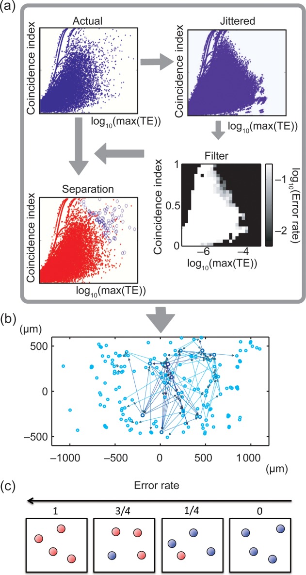
Approach for determining significant connections. (a) First, CI was plotted against log(TE_max) for all neuron pairs from actual data (dots represent pairs). Second, CI was plotted against log(TE_max) for jittered data. Third, both plots were combined to construct a filter that indicated the ratio of jittered dots to all dots in each of the 25 × 25 2D bins (white: many jittered; black: few jittered). Fourth, filter was used to indicate actual connections where jittered pairs were few. Several lines in the distributions occur because when coincident firing happens only once or twice, the TE values become disretized. (b) Connectivity map with actual directional connections plotted as arrows. Thickness indicates strength. Circles represent presumed neuron locations on array. (c) The concept of error rate. The red and blue balls, respectively, represent data samples of jittered data (n = 100) and original data included in a bin. Because error rate is defined as ratio of the number of red balls to the number of all balls, the error rate becomes higher toward the left side in this figure.

Second, we plotted CI values against log₁₀(TE_Pk) values for all possible pairs of neurons within the jittered datasets. When this was done, the jittered data did not extend into the region where both CI and log₁₀(TE_Pk) were simultaneously high (Fig. 2a, “Jittered”), whereas some of the actual data did occupy this region. Intuitively, this region of the plot was populated only by connections with tall and narrow peaks in TE that were unlikely to be the result of common drive (Supplementary Fig. 2b). The upper rightmost portion of the jittered data thus formed a decision boundary that allowed us to distinguish significant connections from those produced by chance. We found that when this CI versus log₁₀(TE_Pk) plot was divided at a resolution of 25 × 25 bins in 2D space, this decision boundary was smooth and closely followed the contours of the jittered data distribution (Fig. 2a, “Separated”). As seen in the figure, the decision boundary between the jittered and actual data forms a curve that is not merely a straight line in either the CI or the log₁₀(TE_Pk) space. Rather, the decision boundary shows a smooth co-variation between these variables, emphasizing that this decision requires 2 variables. The number of 2D bins in this plot was chosen to minimize the squared error between the actual data and the binned histogram, following (Terrell and Scott 1985). Because we observed 2D space, the number of bins needed to be greater than (2n)^1/3 (where n is the number of connections). Because the maximum value of this variable in our data was <20, we selected 25 as the number of bins in each dimension.

In all network studies where actual data are compared with shuffled datasets, it is necessary to select a threshold for significance. To do this, we had to decide which bins in the log₁₀(TE) versus CI plot to include. We did this by measuring what fraction of connections in each bin would come from shuffled data. As we sought to exclude shuffled data, we called this measure the error, E, given by:

$$E(\text{CI},\text{T}{\text{E}}_{\mathrm{pk}})=\frac{N_{\mathrm{jitt}}(\text{CI},\text{T}{\text{E}}_{\mathrm{pk}})}{N_{\mathrm{actual}}(\text{CI},\text{T}{\text{E}}_{\mathrm{pk}})+N_{\mathrm{jitt}}(\text{CI},\text{T}{\text{E}}_{\mathrm{pk}})}.$$ (4)

where the number of data samples at each bin was denoted by N_actual for actual data, and by N_jitt for 100 jittered datasets. This error rate gave the fraction of connections in any bin that came from randomized data. An intuitive, and accurate, explanation is shown in Figure 2c. We identified connections as significant if they occurred in a bin that had an error rate below a chosen threshold. Two criteria motivated the choice of threshold (Fig. 2a, “Filtered”). First, we wanted an error rate that was sufficiently low. As most statistical tests are set with an error rate of 0.05 or lower, we sought a threshold that would be consistent with this. Second, we sought to report network features that were robust with respect to changes in threshold. This motivated us to choose a threshold that was in the middle of a range over which the fraction of significant connections remained relatively constant. We used E = 0.03 as the threshold error rate because the connectivity density is robustly stable around this region (Supplementary Fig. 1e,f). To demonstrate robustness, we also examined how threshold values of E = 0.02 (33% decrease in threshold) and E = 0.04 (33% increase in threshold) affected some network features. Finally, we eliminated connections if TE_Pk was smaller than TE₀ (TE at t = 0) because if TE₀ was bigger than TE_Pk the result indicated that the real peak of TE existed before t = 0. In this case, a causal interaction would have existed from the postconnection neuron to the preconnection neuron, which would be clearly incorrect. This method allowed us to construct networks of effective connectivity from the spike train data (Fig. 2b). We used TE to identify peaks as described above; near these peaks (−3∼−1,1∼3 ms), we looked at whether the cross-correlation was positive or negative. It is known that the shapes of the cross-correlation can sometimes indicate whether a connection is excitatory or inhibitory (Bartho et al. 2004). This analysis showed that 98 ± 1% of the connections showed positive peaks, indicating excitatory connections. Thus, all of the networks presented here are estimated as almost entirely composed of excitatory neurons. Notice that our method is able to infer both excitatory and inhibitory connections; however, due to the skewness of the TE method in detecting excitatory connections, most of the connections considered as significant will belong to excitatory neurons. Further experiments would be required to separate excitatory from inhibitory connections. Although TE can detect inhibitory connections (Ito et al. 2011), this is only possible if excitatory neurons have very high firing rates, so that a reduction in spiking can be detected against a background of high activity. With the firing rates we have here, well below 10 Hz, it is difficult to detect any significant drop in spiking that may be caused by an inhibitory connection. Note that this problem does not exist for TE in detecting excitatory connections, as the addition of a spike is more easily detected against a background of relative silence. Using TE, the number of connections that we identified as coming from inhibitory neurons was very small, and had no appreciable effects on network topology (clusters, communities, hubs).

Clustering

Once significant connections were established, we used several measures to characterize the resulting networks. At the scale of several neurons, we evaluated network clustering properties based on the methods of Perin et al. (2011). Because patch-clamp experiments observe interactions between neurons directly, we expected this comparison would help in making relative comparisons to TE measures. Original figures were provided by Perin et al. (2011). The first comparison involved the histogram of the number of connections for all clusters included in the entire network. The second comparison involved the common neighbor effect (Perin et al. 2011). Common neighbors are nodes simultaneously connecting to 2 already connected neurons. We observed how connectivity probability changed depending on the number of common neighbors.

Network Community

In graph theory terms (Newman 2009), each neuron was considered a node and a connection from one neuron to another was considered a directed edge; the measures we used were for directed graphs. The in-degree of a node was given by the number of connections to the node; the out-degree was given by the number of connections from the node. Hubs were defined as nodes showing high total degree (explained in detail below). The path length was the number of nodes traversed in the shortest path between 2 nodes. The local clustering coefficient was given for nodes in the network, and the average path length was taken over all possible pairs of nodes in the network.

To detect community structures at the scale of tens of neurons, we used modularity (Girvan and Newman 2002; Newman 2004, 2006). The best grouping of community structures was achieved by maximizing the value of modularity, Q, which was given by:

$$Q=\frac{1}{4m}\sum _{ij}\left[A_{ij}-\frac{k_i{k}_j}{2m}\right]\delta (c_i,c_j).$$ (5)

Here, A_ij gave the connection matrix between nodes i and j. This matrix was symmetrized as $A_{ij}=(B_{ij}+B_{ij}^T)/2$ if we express the original matrix as B_ij. In what follows, all variables in community detection analysis were determined from the symmetrized matrix. Here, k_i and k_j were the degree of nodes i and j, and $m=1/2{\sum }_i{k}_i$ was the total number of edges in the network. If nodes i and j belonged to the same community, c, then the delta function δ(c_i,c_j) was 1; otherwise, it was 0. Note that different groupings would affect the value of Q through this delta function. The term $k_i{k}_j/2m$ gave the expected weight of a connection between node i and node j if the network were randomized. Therefore, the term (A_ij−k_ik_j/2m) indicated how much more strongly the actual graph was connected than a random graph. This modularity Q has been successfully applied in whole-brain datasets to understand brain connectomic architecture (Sporns 2013; Shimono 2013), and also applied in spike trains (Humphries 2011). Although there are many methods for detecting communities, this one has been widely used (Fortunato 2010). Note that, in this formulation, each node could only belong to one community. The computational algorithm was based on (Blondel et al. 2008).

Similarity Index of Community Architecture

To quantitatively compare modular structures in unshuffled and shuffled versions of a network, we developed a Similarity index. This index expressed the fraction of nodes placed in the same communities in the original network and in its shuffled counterpart. We defined the similarity index as:

$$\text{Similarity}\text{index}=\frac{1}{N(N-1)}\sum _{i,j}\delta ({\delta }_{\mathrm{NC}1}(i,j),{\delta }_{\mathrm{NC}2}(i,j)).$$ (6)

Equation (6) consists of 2 parts: First, we evaluated whether 2 nodes belonged to the same community using ${\delta }_{\mathrm{NC}1}(i,j)$ and ${\delta }_{\mathrm{NC}2}(i,j)$, where $\delta (i,j)$ was the Kronecker delta function. Accordingly, ${\delta }_{\mathrm{NCn}}(i,j)(n=1,2)$ was 1 when node i belonged to the same community as node j, and was 0 otherwise. We evaluated this for each network architecture. Next, we compared 2 network architectures using another δ function. This δ function was 1 if ${\delta }_{\mathrm{NC}1}(i,j)={\delta }_{\mathrm{NC}2}(i,j)$, and this δ function was 0 if ${\delta }_{\mathrm{NC}1}(i,j)\ne {\delta }_{\mathrm{NC}2}(i,j)$. Briefly, this second delta function checked if the co-participation of node i and j were same or not between unshuffled and shuffled networks. N was the total number of nodes in the network. Thus, the Similarity index normalized the number of co-participating nodes by the total number of pairs of nodes. An example of how this worked is given below (Fig. 3). Network 1 has 2 communities, as does Network 2. The dark gray community has 4 shared nodes between the networks, and the white community has 3 shared nodes between the networks. The total number of pairs where ${\delta }_{\mathrm{NC}1}(i,j)={\delta }_{\mathrm{NC}2}(i,j)$ is given by the number of white boxes in Figure 3b. Thus, the similarity index in this case is [(4 × 4 − 4) + 2 × 3 × 4 + (3 × 3 − 3))/(8 × (8 − 1)] = 42/56 = 3/4. We also analyzed the data using the participation distance instead of similarity index, and obtained similar results (Meila 2007).

Figure 3.

Definition of Similarity index. The main purpose of the Similarity index is to quantify the extent to which 2 community architectures are similar. (a) An example comparing 2 network architectures, 1 and 2. In this case, δ_NC1(i,j) = 0 because nodes i and j participate in 2 different communities in network architecture 1, and δ_NC2(i,j) = 1 because nodes i and j participate in 2 different communities in network architecture 2. Therefore, δ(δ_NC1(i,j),δ_NC2(i,j)) is 0. However, between nodes j and k, δ(δ_NC1(i,j),δ_NC2(i,j)) is 1 because nodes j and k participate in the same community in both network architectures. By summing all pairs of nodes i and j, we can obtain the final value of the Similarity index. (b) A scheme of how to calculate the Similarity index. The x-axis represents network architecture 1, and the y-axis represents network architecture 2. Colors (dark gray or white) correspond to communities shown in (a). Regions where δ_NC1(i,j) = δ_NC2(i,j) are shown as white boxes, and regions where δ_NC1(i,j)≠δ_NC2(i,j) are shown as black boxes. The diagonal components would be self-connections, and are not considered in calculating the Similarity index. Graphically, the Similarity index is defined as (total number of white boxes except diagonal components)/(total number of boxes except diagonal components).

Results

The results are composed of 4 sections. First, we describe general features of cultured cortical slice network activity. Second, we report nonrandom features in connectivity among clusters of up to 6 neurons. Third, we report on community structure and hubs at the scale of tens or more neurons. Fourth, we show how structures at these 2 scales (cluster and community) are related.

General Description of Network Activity

Data were taken from 25 organotypic cultures of cortex recorded for 1.16 ± 0.17 h (mean ± SD). The average number of sorted neurons per culture was 310 ± 127 (mean ± SD), and the average firing rate per neuron was 0.79 ± 0.65 Hz. Network activity typically consisted of a relatively constant background firing rate, punctuated by bursts in which many neurons participated, as previously reported (Tang et al. 2008).

A raster plot of activity illustrating this is shown in Figure 1b. Firing rates remained approximately constant over the duration of the recordings.

Clusters at the Small Scale of up to 6 Neurons

In the next few sections, we use some of the statistical methods developed by Perin et al. (2011) in their patch-clamp studies of connectivity at the scale of up to 6 neurons. These methods allow us to observe structures not only between 2 or 3 neurons (correlations or motifs) but also among clusters of 3 to 6 neurons in a unified framework. In addition, by using these methods, we can compare our connectivity results with those obtained from previous patch-clamp experiments.

Figure 4a shows the number of connections actually observed (sold lines) plotted with the number of connections expected by chance (dotted lines) in clusters of 3 neurons. The expected value was calculated from the number of separated pairs, monodirectional connections, and bidirectional connections included in the network organization (Perin et al. 2011).

Figure 4.

High numbers of connections occur more than chance in clusters of up to 6 neurons. Each plot shows how often a given number of connections occurred for clusters of up to 6 neurons. Curves of dotted lines show connections expected by chance. In chance shuffling, the numbers of directed inputs, directed outputs, and bidirectional connections was preserved. Curves of sold lines show connections observed in data. In general, solid lines tended to depart from dotted lines at high numbers of connections, suggesting nonrandomness of connections. Top row (a–d) shows results for networks constructed from effective connectivity (TE); bottom row (e–h) shows results for networks constructed from patch-clamp experiments (synaptic connections; Perin et al. 2011). Small networks inset in (a–d) show schematic example clusters. Number of neurons in each cluster goes from 3 (left) to 6 (right). Note qualitative similarity between effective connections measured by TE and synaptic connections assessed by patch-clamp. Larger groups of neurons tended to have more connections than chance (*P < 0.01, **P < 0.001; z-test).

Clusters of 3 neurons were found to have 4 connections among them significantly more often than expected by chance. For larger clusters of neurons, the differences between actual and expected numbers of connections were even greater at higher numbers of connections (Fig. 4b,c,d) (*P < 0.01, **P < 0.001; z test). For comparison, we have shown the results from the patch-clamp study by Perin et al. (2011) in Figure 4d,e,f. Despite the fact that these 2 datasets were collected in markedly different preparations (organotypic cultures or acute slices), there was substantial qualitative similarity. In both datasets, dense connectivity in clusters of neurons occurred more often than expected by chance, and this tendency increased with the number of neurons in the cluster.

We next examined how the probability of an effective connection between pairs of neurons was influenced by the presence of common neighbors. Perin et al. found 2 main things: First, at all distances, the probability of a unidirectional connection between 2 neurons was greater than the probability of a bidirectional connection. Second, the probability of connectivity increased approximately linearly with the number of common neighbors. The histogram in Figure 5a shows the effective connection probability for pairs of neurons that shared (open bars) and did not share (filled bars) a common neighbor. Results are binned in 50-μm intervals as a function of distance between the 2 connected neurons. Neurons with a common neighbor had significantly higher connection probabilities than neurons without a neighbor at all distances (Fig. 5a, *P < 0.01, t-test). Furthermore, when there was more than one common neighbor, the connection probability was also significantly increased (*P < 0.01, t-test). The plot in Figure 5b shows both the observed (open circles) and expected (filled circles) connection probability between pairs of neurons for different numbers of common neighbors. The probability of an effective connection also increased approximately linearly with the number of common neighbors, and this effect was statistically significant for all numbers of common neighbors examined (R = 0.94, P < 0.01). For comparison, the results from the patch-clamp studies of Perin et al. are also plotted in Figure 5c,d. Here, there was a significant common neighbor effect at all distances tested, and there was qualitative similarity with the effective connectivity results (R = 0.94, P < 0.01). In addition, for both this patch-clamp method and our effective connectivity method, connection probability increased almost linearly with the number of common neighbors. In addition, we have examined whether or not the results reported here are robust with respect to errors in spike sorting, and found that randomly injected or deleted spikes did not influence common neighbor effects (Supplementary Fig. 4). In addition, these results did not depend sharply on the error threshold, as common neighbor effects and connectivity statistics among clusters of 3–6 neurons remained qualitatively similar for different thresholds (Supplementary Fig. 5). To what extent do our results implicate hubs beyond the fact that they have a large number of connections? Indeed, we found that shuffling the same number of connections among nonhub neurons also disrupted structure at both scales examined. However, this process involved a much larger number of neurons. Because of their concentrated connections, the loss of only a few hub neurons would substantially disrupt structure at both scales. Our findings indicate that this is only a result of their large number of connections.

Figure 5.

Common neighbors increase probability of further connections. (a) Probability of an effective connection (from TE) as a function of distance for pairs that share a common neighbor (filled bars) and those that do not (open bars). Error bars are SEMs of 10 data samples (*P < 0.01, t-test). (b) Probability of an effective connection (from TE) between 2 neurons as a function of different numbers of common neighbors. Solid line is the best fit line from data. Dotted line is best fit line for chance expected values. The expected values were given how many common neighbors will be observed just when given the connectivity probability of the real data. Error bars are SEMs of 9 data samples. For comparison, (c) and (d) show same analyses applied to synaptic connectivity assessed by patch-clamp (Perin et al. 2011).

Larger Scale Network Structures: Communities and Hubs

We next shifted our focus to results at the scale of tens of neurons simultaneously recorded. Here we were no longer able to compare our effective connectivity findings with those obtained from patch-clamp experiments, as the maximum number of neurons reported to have been simultaneously sampled with patch-clamp techniques was about 12 (Perin et al. 2011). The large samples of 100 or more neurons that we recorded with extracellular electrodes allowed us to apply a community detection algorithm (Blondel et al. 2008). With this algorithm, nodes were provisionally integrated into different numbers of communities. The integration that maximized the modularity score was used to determine the number of communities. Recall that modularity measured the extent to which neurons within a community were more connected than expected by chance.

Figure 6a shows how the neurons in 3 representative networks (of 25) were spatially located, with the outline of the 512 electrode array indicated by the black rectangles. Different markers of nodes indicate different community memberships. Effective connections are shown as colored arrows. Visual inspection immediately suggested that network architecture could range from 2 separated communities (the rightmost example in Fig. 6a or Fig. 7f) to large integrated communities (the leftmost example in Fig. 6a or the left panel of Fig. 7e). Similar figures, including more information, are shown again in Figure 7e,f. Figure 6b shows how each of the networks in Figure 6a were partitioned into communities. The y-axis indicates the percentage of neurons that were included in each community, and the x-axis indicates the community number, arranged in descending order of size. For the leftmost network, nearly 80% of the neurons were contained in one community; the remaining communities each included no more than 7% of the neurons. This was a highly integrated network. For the rightmost network, the largest communities each contained roughly 40% of the neurons and the second largest community contained 20% of the neurons. The most typical result was the network in the middle panel, which showed one large community and one medium or small community.

Figure 6.

Large-scale structure of networks. (a) Spatial locations of neurons recorded from the rectangular electrode array, with effective connections shown. The 3 networks represent the breadth of community structures found. These 3 networks are shown at figure 7(e) and (f) with colored and zoomed. (b) Percentage of neurons included in communities plotted against number of communities, for the 3 networks. (c) Average percentage of neurons included in communities plotted against number of communities. Note that, on average, only 2 communities were needed to encompass over 95% of neurons (*P < 0.01, **P < 0.001). (d) Distribution of neuron degrees, plotted in log–log space. The dotted line is for out-degree, the solid line is for in-degree. Note fat tail of distribution, different from chance expectation. (e) Distance between neurons plotted against path length. Path length tended to increase with distance linearly. The error bars are standard deviation among slices.

Figure 7.

Hubs and their connections can affect connectivity statistics at small and large scales. (a) Upper 4 panels show frequency distributions of connections for clusters of 3–6 neurons (as in Fig. 4) after exchanging connections from 1 to 6% of high-degree nodes with connections from 1 to 6% of low-degree nodes. Line color indicates extent of shuffling. Colored lines are above dashed lines, indicating that number of connections in small neuron groups exceeded chance levels. Note that increased amounts of shuffling (lighter colors) caused the curves to fall toward chance levels. The shaded panels below these graphs show the probability of observing each number of connections for a given neuron group size. Percentage shuffled is on the y-axis, number of connections is on the x-axis, and probability is given by shading, with darker representing less probable. Note that least probable connections tend to occur with lowest amounts of shuffling, and that larger numbers of connections are less probable. The red dashed line indicates the number of connections that was found to be least probable for a given neuron group size. (b) A comparison of P-values obtained from shuffling connections of hub neurons. These P-values were given at sections shown by red dotted lines in lower panels in (a). Curves in all cases move upward for larger amounts of shuffling, indicating loss of structure. Note that significant loss of small-scale structure is occurs after shuffling only 1% of hub neurons. (c) Dissolution of community structure by shuffling of hubs. y-Axis is similarity of shuffled community structure to that found in data; x-axis is percentage of hubs used for shuffling. (d) P-values for community structure as a function of shuffling. Again, note that both curves move upward for increased amounts of shuffling, indicating loss of structure at large scale. Note that the percentage at which the large-scale structure was significantly lost (6%) was clearly larger than the percentage at which the small-scale structure was significantly lost (1%). (e) and (f) Spatial locations of hub neurons on the rectangular electrode array are shown as yellow markers, indicating that they could be found both in the center of the array as well as on the edges. (f) The 3 network features (hub, cluster and community) of various scales that we have examined. Translucent red and blue regions cover 2 large communities, which can also be identified by different node symbols (small orange circles or squares). The translucent yellow region covers a representative cluster of 6 neurons.

Continuing with large-scale network structure, Figure 6d shows the average degree distribution of all 25 datasets. It was clearly not Gaussian and had a long tail, consistent with findings in macroscopic brain networks. This result made it reasonable for us to identify hubs as a very small subpopulation of nodes with degrees much higher than average. Figure 6e shows the relationship of physical distance between neurons and their average path lengths for all data. Recall that the path length between 2 neurons is the least number of connections that must be traversed in going from one neuron to the other. There was a clear trend for physical distance to monotonically increase with path length. These results indicated that the long-tailed degree distribution was actually embedded in the spatial extent of the multielectrode array. This is in contrast to many degree distributions that have little or no spatial embedding (e.g., Shiffrin and Börner 2004; Ugander et al. 2011). In addition, how the distance changed depending on relative delay is shown in Supplementary Figure 7. These large-scale network features could only be observed from data collected simultaneously from hundreds of closely spaced recording sites, processed at high temporal resolution. There was a weak correlation between degree and firing rate (CC ∼0.2, P > 0.1).

Influence of Hub Nodes on Structure at 2 Different Scales

After nonrandom structure at 2 different scales had been identified, we next sought to explore factors that could affect structure at these scales. A natural candidate for this role was hub neurons because of their many connections to small groups of neurons as well as to larger communities of neurons. Our approach was to swap connections of the highest degree (hub) neurons with connections of the lowest degree neurons. We would then examine whether or not this swapping significantly changed structure observed at the 6 neuron scale as well as structure observed at the scale of tens or more neurons. We started out swapping with a small percentage of hub neurons, 1%, and increased up to 10%. In each of these swaps, we also counted the total number of connections that were exchanged. The results of this swapping are presented in Figure 7. Panels (a) and (b) show the effects of swapping on connections in clusters of up to 6 neurons, whereas panels (c) and (d) show the effects of swapping on the existence of communities at the scale of tens or more neurons. The overall result is that swapping eventually destroys the nonrandom structure observed at each scale. However, the amount of swapping needed to destroy structure differs depending on scale.

We will first describe the results of swapping on cluster structure. The dashed lines in Figure 7a show the number of connections expected by chance in clusters of 6 neurons, and the colored lines show the number of connections observed for swapping in different percentages of high-degree nodes. Note that as the percentage of high-degree nodes that experienced swapping was increased, the blue lines shifted downward, eventually becoming indistinguishable from the dashed line. This showed how swapping gradually made the observed structures fade away to only chance levels. The statistical tests in the lower panels of Figure 7a showed the contour map of P-values when changing the shuffling percentages. Recall that high P-values indicate structures not different from chance. In order to observe the trend easily, we plotted the representative change of P-values under red dotted lines in the lower panels of Figure 7a as Figure 7b. We selected these points because the P-values were minimal there before shuffling was done. We sought to determine if this degradation of structure in clusters was produced by hubs specifically, or by the number of connections that hubs had. Figure 7b shows how increased amounts of exchanging connections from high-degree nodes gradually caused P-values to climb to chance levels. From these results, we found that structure in clusters of up to 6 neurons was dependent on only 1% of the highest degree neurons. However, the percentage of connections that were involved in this manipulation was surprisingly small, because <10% of all connections were associated with the top 1% of hub neurons.

Turning now to larger scale structure, Figure 7c summarizes the effects of exchanging connections from high-degree nodes on communities. To assess how much community structure changed after exchanging connections, we used the network similarity metric described in the methods section. This told us how similar the resulting community structure was to that originally found in the data. Note the downward slope in Figure 7c, indicating that larger percentages of exchanges caused similarity to decline Figure 7d is another view of this result, here given as a plot of P-values for increasing amounts of shuffle. The curve climbs to nonsignificant levels after connections from 6% of high-degree nodes are exchanged. These results showed that large-scale community structure was dependent on the connections from 6% of the highest degree neurons. It is important to note that the percentage of hub neurons required for disruption here was clearly larger than the 1% needed to disrupt structures in clusters at the 6 neuron scale. In addition, we found a similar result even when we exchanged the same number of connections at randomly selected locations (not at hubs) throughout the network (Supplementary Fig. 3). This suggested that the difference in fragility between clusters and communities could not be attributed to the idea that connections around hub neurons dominate small clusters. To further examine neurons from the upper 6% of the degree distribution, we plotted their locations on the electrode array as yellow circles in Figure 7e. The 3 example networks are representative, and indicate that there was no obvious trend in their locations. Such hub neurons could occur both in the central regions of the array as well as on its edges.

Taken together, these results suggested that the percentages of hub neurons contributing to connectivity statistics observed at the 3–6 neuron scale and at the scale of tens of neurons were relatively small, but clearly different. Because nonrandomness at the scale of tens or more neurons was sustained even after nonrandomness at the 3–6 neuron scale was disrupted, it appears that the structure found at the 36 neuron scale was not necessary for the structure found at the tens of neurons scale. In addition, we also observed this trend in clusters of 7, 8, 10, 12, 18 neurons (Supplementary Fig. 6). Although the percentage of hubs necessary to disrupt clusters gradually increased, the percentage necessary was <4% even in clusters of 18 neurons.

Discussion

Summary of Main Findings

The main findings of this work are fourfold. First, the nonrandom connectivity structure we observed in clusters of up to 6 neurons showed qualitative correspondence with a previous patch-clamp study, lending validity to our methods. Second, from a technical standpoint, this work emphasizes the importance of simultaneous recordings from hundreds of neurons. Third, simultaneous recording enabled us to identify nonrandom features of hubs and communities (Fig. 7f). Fourth, by using 3 “actors” (hubs, clusters, and communities), we demonstrated that structure at the scale of clusters was relatively less robust than structure at the scale of communities.

Influences Between Scales

Previous work by Perin et al. (2011) simulated what would happen if the patterns of synaptic connectivity observed among clusters of up to 6 neurons were embedded randomly in much larger neuronal populations. Their extrapolation showed that nonrandomness at the 6 neuron scale naturally generated larger scale groups containing tens of neurons (communities). From this result, Perin et al. suggested that the existence of small-scale nonrandom structure was a sufficient condition to generate larger scale nonrandom structure. Our findings do not contradict their simulation results. We observed that structure at the 6 neuron scale could be disrupted by swapping connections from 1% of the most well-connected neurons; structure at the scale of tens of neurons could be disrupted by swapping connections from 6% of the most well-connected neurons. Thus, although small-scale structure was not a necessary condition for the existence of large-scale structure, substantial disruption produced at the small-scale (by swapping connections from 6% of the most well-connected neurons) would indeed be sufficient to produce disruption at the large scale. Perin et al. also reported a distribution of community sizes, with a median near ∼50 neurons (Perin et al. 2011). How does this relate to our findings? We also observed communities of tens of neurons, but caution should be exercised before using our results to estimate community sizes. Any estimation of community size from our work is inherently limited by the size and geometry of our electrode array. For example, although a community of 200 neurons could be present in a given network, we would only be able to observe it if the array happened to be placed over all the neurons in this community.

Definition and Functional Role of “Hub” Neurons

This study used highly connected hub neurons to quantify differences in fragility between structure at 2 scales. Here, hubs were defined simply based on their relatively high number of connections, as quantified by being in the upper 1%–10% of the degree distribution. In the wider scope of graph theory, we can also regard node degree as one measure that characterizes centrality, or the extent to which a node is located near a central position in its relationships to other nodes. In this generalization, it is also possible to use other centrality measures instead of degree to characterize the central position of hubs in network organization (Sporns et al. 2007; Newman 2009). Furthermore, we can potentially detect “connector hubs” between different communities, which may play important roles for mediating communications between nodes participating in different communities. Our definition of “hub” was based on clear commonalities that hubs are among the most well connected in a given network. The high-degree nodes naturally represent the highly centralized property of hubs characterizing the specific network organization because the degree distribution of our data was long-tailed. As a natural extension, these varieties and subcategories of hubs will be an interesting topic in future studies. Experimentally, selective excitations or depressions of hub neurons by external stimulation could also reveal more specific functional roles for hub neurons in the functional microconnectome.

Validity

An issue of potential concern is that these studies were conducted in organotypic cultures, rather than in acute slices or in vivo. Although such cultures have been previously reported to preserve the gross patterns of anatomical connectivity found in vivo (Gotz and Boltz 1992; Leiman and Seil 1986), as well as many of the emergent firing patterns (Plenz and Kitai 1996, 1998; Beggs and Plenz 2003; Johnson and Buonomano 2007), caution should be used before extrapolating our findings to the intact brain. Despite this caveat, it is interesting to note that the network structures we identified with effective connectivity in slice cultures at the scale of 3–6 neurons had qualitative similarity to the structures identified with synaptic connectivity in acute cortical slices by Perin et al. (2011). Another potential concern is the process by which we selected the parameters for determining significant connections. As described in the Materials and Methods and in Supplementary Figure 1, we have tried to define necessary parameters from natural features of the neuronal activity itself (e.g., where peaks occur, where there is a stable region). We have also sought parameters that would produce results that are robust with respect to changes. Although we chose to maintain a high signal-to-noise ratio, we would like to point out that lowering this requirement, and therefore admitting more connections, would still preserve many of the topological features observed here. How much we can detect weaker connections in the “sea” of noise will be an important future topic that goes beyond the trade-off between the false-positive and true-negative detections.

Relation to Other Work

Many complex networks exhibit modular organization. Of particular interest is how structures within a network relate. For example, the modules (communities) of structural networks in monkey cortex have been related to the nonuniform distribution of neurons (Shimono 2013). Studies of activity in networks containing tens to hundreds of neurons have shown the presence of hubs in hippocampus (Bonifazi et al. 2009), and suggested small-world (Yu et al. 2008) or scale-free (Eytan and Marom 2006) topologies of functional connections in cortex. The present work builds on these previous studies by identifying distinct functional network structures at different scales and takes a first step toward understanding how structures at these different scales relate through hubs.

The present work also offers a new way to view connectivity in cortical circuits that is not highly labor intensive. Previous work has explored the pattern of synaptic connections at the level of a few neurons (Bock et al. 2011; Briggman et al. 2011). These studies have laid an excellent foundation for our wider understanding of connectivity patterns in the brain. Because these structural connectivity studies require intensive labor, they are typically performed on a select set of neurons, and currently cannot provide information about how hundreds of neurons are connected. In this study, we have sought to explore how populations of a hundred or more neurons share activity. The knowledge about directed functional connectivity will be also valuable in revealing ways in which neurons typically share information on their underlying network of structural connections.

On a different topic, we would also like to point out that the intensities of TE approximately follow a lognormal distribution (Supplementary Fig. 2a). Interestingly, this is consistent with previous studies of synaptic strengths found by patch-clamp studies in acute slices (Song et al. 2005; Koulakov et al. 2009), as reviewed in (Buzsaki and Mizuseki 2014). This point of contact will provide new opportunities for future studies. The present work looks at only one aspect of what might be called the cortical microconnectome.

Possible Mechanisms

By what process could hubs come to be situated between structures at 2 scales? Spike-timing-dependent plasticity (STDP) is a natural candidate mechanism. At small scales, simulations have shown that STDP can promote a “rich get richer” dynamics (Zheng et al. 2013). This could lead to the increased clustering of connections seen in groups of 3–6 neurons (see also Yassin et al. 2010). At larger scales, simulations have shown that STDP and Hebb-like (Hebb 1949) plasticity rules can produce competition between neuronal groups (Song and Abbott 2001; Izhikevich et al. 2004; Rubinov et al. 2011). For example, when 2 neurons project with equal strength to the same postsynaptic neuron, small differences in coincident firing will, through positive feedback, cause one connection to become stronger at the expense of the other (Song et al. 2000). This symmetry breaking is thought to be at work in competition within cortical somatosensory maps after nerve sectioning (Merzenich et al. 1983). In this manner, STDP could lead to the formation of different communities of neurons, as observed in our data. It is also possible that genetic factors could play a role in specifying hub neurons, but this is beyond the scope of the present paper. Future experiments could investigate the role of these hub neurons in percolation (Eckmann et al. 2008) or in activity initiation (Eckmann et al. 2010).

Concluding Remarks

The present work has demonstrated that networks of spiking neurons display specific nonrandom structures at different scales. It has also explored how nonrandomness at different scales (hubs, clusters, and communities) is related. The investigation of how these structures change after randomization suggests that robustness may differ across scales. How features in the millimeter scale can be compared and combined with features in macroscopic anatomies (Shimono 2013, 2014; Scholtens et al. 2014) and dynamics to understand cognitive behaviors, which neuronal substrates were observed in one particular scale before (e.g., Shimono et al. 2007, 2011, 2012; Shimono and Niki 2013; Nakhnikian et al. 2014), more completely will be also essentially important topic for future neuroscience.

Supplementary Material

Supplementary material can be found at: http://www.cercor.oxfordjournals.org/.

Funding

This study was supported by funding for JSPS Research Abroad to M.S. from MEXT (The Ministry of Education, Culture, Sports, Science, and Technology), funding from NSF (grant numbers 0904912 and 1058291) to J.M.B. Funding to pay the Open Access publication charges for this article was provided by JSPS Research Abroad to M.S. from MEXT (The Ministry of Education, Culture, Sports, Science, and Technology).

References

- Aertsen AM, Gerstein GL, Habib MK, Palm G. 1989. Dynamics of neuronal firing correlation: modulation of “effective connectivity”. J Neurophysiol. 61(5):900–917. [DOI] [PubMed] [Google Scholar]
- Baker RE, Corner MA, van Pelt J. 2006. Spontaneous neuronal discharge patterns in developing organotypic mega-co-cultures of neonatal rat cerebral cortex. Brain Res. 1101(1):29–35. [DOI] [PubMed] [Google Scholar]
- Baker RE, van Pelt J. 1997. Co-cultured but not isolated cortical explants display normal dendritic development: a long-term quantitative study. Dev Brain Res. 98:21–27. [DOI] [PubMed] [Google Scholar]
- Bartho P, Hirase H, Moncoduit L, Zutaro M, Harris KD, Buzsaki G. 2004. Characterization of neocortical principal cells and interneurons by network interactions and extracellular features. J Neurophysiol. 92:600–608. [DOI] [PubMed] [Google Scholar]
- Bar-Yam Y. 2004. Multiscale variety in complex systems. Complexity. 9(4):37–45. [Google Scholar]
- Bassett DS, Brown JA, Deshpande V, Carlson JM, Grafton ST. 2011. Conserved and variable architecture of human white matter connectivity. Neuroimage. 54(2):1262–1279. [DOI] [PubMed] [Google Scholar]
- Bassett DS, Meyer-Lindenberg A, Achard S, Duke T, Bullmore E. 2006. Adaptive reconfiguration of fractal small-world human brain functional networks. Proc Natl Acad Sci USA. 103(51):19518–19523. [DOI] [PMC free article] [PubMed] [Google Scholar]
- Beggs JM, Plenz D. 2004. Neuronal avalanches are diverse and precise activity patterns that are stable for many hours in cortical slice cultures. J Neurosci. 24(22):5216–5229. [DOI] [PMC free article] [PubMed] [Google Scholar]
- Beggs JM, Plenz D. 2003. Neuronal avalanches in neocortical circuits. J Neurosci. 23:11167–11177. [DOI] [PMC free article] [PubMed] [Google Scholar]
- Berry MS, Pentreath VW. 1976. Criteria for distinguish between monosynaptic and polysynaptic transmission. Brain Res. 105:1–20. [DOI] [PubMed] [Google Scholar]
- Biswal B, Zerrin Yetkin F, Haughton VM, Hyde JS. 1995. Functional connectivity in the motor cortex of resting human brain using echo - planar mri. Magn Reson Med. 34(4):537–541. [DOI] [PubMed] [Google Scholar]
- Blondel VD, Guillaume JL, Lambiotte R, Lefebvre E. 2008. Fast unfolding of communities in large networks. J Stat Mech Theory Exp. 2008(10):P10008. [Google Scholar]
- Bock D, Lee W-C, Kerlin AM, Andermann ML, Yurgenson S, Hood G, Wetzel AW, Soucy E, Kim HS, Reid RC. 2011. Network anatomy and in vivo physiology of a group of visual cortical neurons. Nature. 471:177–182. [DOI] [PMC free article] [PubMed] [Google Scholar]
- Bolz J, Novak N, Gotz M, Bonhoeffer T. 1990. Formation of target-specific neuronal projections in organotypic slice cultures from rat visual-cortex. Nature. 346(6282):359–362. [DOI] [PubMed] [Google Scholar]
- Bonifazi P, Goldin M, Picardo MA, Jorquera I, Cattani A, Bianconi G, Represa A, Ben-Ari Y, Cossart R. 2009. GABAergic hub neurons orchestrate synchrony in developing hippocampal networks. Science. 326(5958):1419–1424. [DOI] [PubMed] [Google Scholar]
- Briggman KL, Helmstaedter M, Denk W. 2011. Wiring specificity in the direction-selectivity circuit of the retina. Nature. 471(7337):183–188. [DOI] [PubMed] [Google Scholar]
- Buonomano DV. 2003. Timing of neural responses in cortical organotypic slices. Proc Natl Acad Sci USA. 100(8):4897–4902. [DOI] [PMC free article] [PubMed] [Google Scholar]
- Buzsáki G, Mizuseki K. 2014. The log-dynamic brain: how skewed distributions affect network operations. Nat Rev Neurosci. 15:267–278. [DOI] [PMC free article] [PubMed] [Google Scholar]
- Caeser M, Bonhoeffer T, Bolz J. 1989. Cellular organization and development of slice cultures from rat visual cortex. Exp Brain Res. 77(2):234–244. [DOI] [PubMed] [Google Scholar]
- Carlson JM, Doyle J. 2002. Complexity and robustness. Proc Natl Acad Sci USA. 99(Suppl 1):2538–2545. [DOI] [PMC free article] [PubMed] [Google Scholar]
- Chiappalone M, Bove M, Vato A, Tedesco M, Martinoia S. 2006. Dissociated cortical networks show spontaneously correlated activity patterns during in vitro development. Brain Res. 1093:41–53. [DOI] [PubMed] [Google Scholar]
- Dodds PS, Watts DJ, Sabel CF. 2003. Information exchange and the robustness of organizational networks. Proc Natl Acad Sci USA. 100(21):12516–12521. [DOI] [PMC free article] [PubMed] [Google Scholar]
- Eckmann JP, Jacobi S, Marom S, Moses E, Zbinden C. 2008. Leader neurons in population bursts of 2D living neural networks. New J Phys. 10:5011. [Google Scholar]
- Eckmann JP, Moses E, Stetter O, Tlusty T, Zbinden C. 2010. Leaders of neuronal cultures in a quorum percolation model. Front Comput Neurosci. 4:132. [DOI] [PMC free article] [PubMed] [Google Scholar]
- Eytan D, Marom S. 2006. Dynamics and effective topology underlying synchronization in networks of cortical neurons. J Neurosci. 26(33):8465–8476. [DOI] [PMC free article] [PubMed] [Google Scholar]
- Field GD, Gauthier JL, Sher A, Greschner M, Machado TA, Jepson LH, Shlens J, Gunning D, Mathieson K, Paninski L, et al. 2010. Functional connectivity in the retina at the resolution of photoreceptors. Nature. 467:673–677. [DOI] [PMC free article] [PubMed] [Google Scholar]
- Fortunato S. 2010. Community detection in graphs. Phys Rep. 486:75–174. [Google Scholar]
- Friedman N, Ito S, Brinkman BAW, Shimono M, DeVille REL, Dahmen KA, Beggs JM, Butler TC. 2012. Universal critical dynamics in high resolution neuronal avalanche data. Phys Rev Lett. 108:208102. [DOI] [PubMed] [Google Scholar]
- Friston KJ. 2011. Functional and effective connectivity: a review. Brain Connect. 1(1):13–36. [DOI] [PubMed] [Google Scholar]
- Friston KJ. 1994. Functional and effective connectivity in neuroimaging: a synthesis. Hum Brain Mapp. 2:56–78. [Google Scholar]
- Garofalo M, Nieus T, Massobrio P, Martinoia S. 2009. Evaluation of the performance of information theory-based methods and cross-correlation to estimate the functional connectivity in cortical networks. PLoS One. 4(8):e6482. [DOI] [PMC free article] [PubMed] [Google Scholar]
- Gireesh ED, Plenz D. 2008. Neuronal avalanches organize as nested theta- and beta/gamma-oscillations during development of cortical layer 2/3. Proc Natl Acad Sci USA. 105(21):7576–7581. [DOI] [PMC free article] [PubMed] [Google Scholar]
- Girvan M, Newman ME. 2002. Community structure in social and biological networks. Proc Natl Acad Sci USA. 99(12):7821–7826. [DOI] [PMC free article] [PubMed] [Google Scholar]
- Gotz M, Bolz J. 1992. Formation and preservation of cortical layers in slice cultures. J Neurobiol. 23(7):783–802. [DOI] [PubMed] [Google Scholar]
- Gourevitch B, Eggermont JJ. 2007. Evaluating information transfer between auditory cortical neurons. J Neurophysiol. 97(3):2533–2543. [DOI] [PubMed] [Google Scholar]
- Harris-White ME, Zanotti SA, Frautschy SA, Charles AC. 1998. Spiral intercellular calcium waves in hippocampal slice cultures. J Neurophysiol. 79(2):1045–1052. [DOI] [PubMed] [Google Scholar]
- Hebb DO. 1949. The organisation of behaviour: a neuropsychological theory. Psychology Press. [Google Scholar]
- Hlavá˘cková-Schindler K, Paluš M, Vejmelka M, Bhattacharya J. 2007. Causality detection based on information-theoretic approaches in time series analysis. Phys Rep. 441(1):1–46. [Google Scholar]
- Humphries MD. 2011. Spike-train communities: finding groups of similar spike trains. J Neurosci. 31(6):2321–2336. [DOI] [PMC free article] [PubMed] [Google Scholar]
- Ikegaya Y, Aaron G, Cossart R, Aronov D, Lampl I, Ferster D, Yuste R. 2004. Synfire chains and cortical songs: temporal modules of cortical activity. Science. 304(5670):559–564. [DOI] [PubMed] [Google Scholar]
- Ito S, Hansen M, Heiland R, Lumsdaine A, Litke A, Beggs JM. 2011. Extending transfer entropy improves identification of effective connectivity in a spiking cortical network model. PLoS One. 6(11):e27431. [DOI] [PMC free article] [PubMed] [Google Scholar]
- Izhikevich EM, Gally JA, Edelman GM. 2004. Spike-timing dynamics of neuronal groups. Cereb Cortex. 14:933–944. [DOI] [PubMed] [Google Scholar]
- Johnson HA, Buonomano DV. 2007. Development and plasticity of spontaneous activity and Up states in cortical organotypic slices. J Neurosci. 27(22):5915–5925. [DOI] [PMC free article] [PubMed] [Google Scholar]
- Juergens E, Eckhorn R. 1997. Parallel processing by a homogeneous group of coupled model neurons can enhance, reduce and generate signal correlations. Biol Cybern. 76(3):217–227. [DOI] [PubMed] [Google Scholar]
- Klostermann O, Wahle P. 1999. Patterns of spontaneous activity and morphology of interneuron types in organotypic cortex and thalamus–cortex cultures. Neuroscience. 92(4):1243–1259. [DOI] [PubMed] [Google Scholar]
- Koulakov AA, Hromádka T, Zador AM. 2009. Correlated connectivity and the distribution of firing rates in the neocortex. J Neurosci. 29(12):3685–3694. [DOI] [PMC free article] [PubMed] [Google Scholar]
- Leergaard TB, Hilgetag CC, Sporns O. 2012. Mapping the connectome: multi-level analysis of brain connectivity. Front Neuroinformatics. 6(14):1–5. [DOI] [PMC free article] [PubMed] [Google Scholar]
- Leiman AL, Seil FJ. 1986. Influence of subcortical neurons on the functional development of cerebral neocortex in tissue culture. Brain Res. 365(2):205–210. [DOI] [PubMed] [Google Scholar]
- Lindner M, Vicente R, Priesemann V, Wibral M. 2011. TRENTOOL: a Matlab open source toolbox to analyse information flow in time series data with transfer entropy. BMC Neurosci. 12(1):119. [DOI] [PMC free article] [PubMed] [Google Scholar]
- Litke AM, Bezayiff N, Chichilnisky EJ, Cunningham W, Dabrowski W, Grillo AA, Grivich M, Grybos P, Hottowy P, Kachiguine S, et al. 2004. What does the eye tell the brain? Development of a system for the large-scale recording of retinal output activity. IEEE Trans Nucl Sci. 51(4):1434–1440. [Google Scholar]
- Lungarella M, Pitti A, Kuniyoshi Y. 2007. Information transfer at multiple scales. Phys Rev E. 76:0561171–05611710. [DOI] [PubMed] [Google Scholar]
- Mason A, Nicoll A, Stratford K. 1991. Synaptic transmission between individual pyramidal neurons of the rat visual cortex in vitro. J Neurosci. 11(1):72–84. [DOI] [PMC free article] [PubMed] [Google Scholar]
- Meil˘a M. 2007. Comparing clusterings—an information based distance. J Multivariate Anal. 98(5):873–895. [Google Scholar]
- Merzenich MM, Kaas JH, Wall J, Nelson RJ, Sur M, Felleman D. 1983. Topographic reorganization of somatosensory cortical areas 3b and 1 in adult monkeys following restricted deafferentation. Neuroscience. 8(1):33–55. [DOI] [PubMed] [Google Scholar]
- Meunier D, Lambiotte R, Fornito A, Ersche KD, Bullmore ET. 2009. Hierarchical modularity in human brain functional networks. Front Neuroinformatics. 3:37. [DOI] [PMC free article] [PubMed] [Google Scholar]
- Nakhnikian A, Rebec GV, Grasse LM, Dwiel LL, Shimono M, Beggs JM. 2014. Behavior modulates effective connectivity between cortex and striatum. PLoS One. 9(3):e89443. [DOI] [PMC free article] [PubMed] [Google Scholar]
- Newman ME. 2004. Fast algorithm for detecting community structure in networks. Phys Rev E. 69(6):066133. [DOI] [PubMed] [Google Scholar]
- Newman ME. 2006. Modularity and community structure in networks. Proc Natl Acad Sci USA. 103(23):8577–8582. [DOI] [PMC free article] [PubMed] [Google Scholar]
- Newman ME. 2009. Networks: an introduction. Oxford: Oxford University Press. [Google Scholar]
- Orlandi JG, Stetter O, Soriano J, Geisel T, Battaglia D. 2013. Transfer entropy reconstruction and labeling of neuronal connections from simulated calcium imaging. ArXiv preprint ArXiv: 1309.4287. [DOI] [PMC free article] [PubMed]
- Pajevic S, Plenz D. 2009. Efficient network reconstruction from dynamical cascades identifies small-world topology of neuronal avalanche. PLoS Comput Biol. 5(1):e1000271. [DOI] [PMC free article] [PubMed] [Google Scholar]
- Paxinos G, Watson C. 2007. The rat brain in stereotaxic coordinates. 6th ed San Diego: Academic Press. [Google Scholar]
- Perin R, Berger TK, Markram H. 2011. A synaptic organizing principle for cortical neuronal groups. Proc Natl Acad Sci USA. 108(13):5419–5424. [DOI] [PMC free article] [PubMed] [Google Scholar]
- Plenz D, Aertsen A. 1996. Neural dynamics in cortex-striatum co-cultures—I. anatomy and electrophysiology of neuronal cell types. Neuroscience. 70(4):861–891. [DOI] [PubMed] [Google Scholar]
- Plenz D, Kitai ST. 1996. Generation of high-frequency oscillations in local circuits of rat somatosensory cortex cultures. J Neurophysiol. 76:4180–4184. [DOI] [PubMed] [Google Scholar]
- Plenz D, Kitai ST. 1998. “Up” and “down” states in striatal medium spiny neurons simultaneously recorded with spontaneous activity in fastspiking interneurons studied in cortex–striatum–substantia nigra organotypic cultures. J Neurosci. 18:266–283. [DOI] [PMC free article] [PubMed] [Google Scholar]
- Rubinov M, Sporns O, Thivierge JP, Breakspear M. 2011. Neurobiologically realistic determinants of self-organized criticality in networks of spiking neurons. PLoS Comput Biol. 7(6):e1002038. [DOI] [PMC free article] [PubMed] [Google Scholar]
- Schneidman E, Berry MJ, Segev R, Bialek W. 2006. Weak pairwise correlations imply strongly correlated network states in a neural population. Nature. 440(7087):1007–1012. [DOI] [PMC free article] [PubMed] [Google Scholar]
- Scholtens LH, Schmidt R, de Reus MA, van den Heuvel MP. 2014. Linking macroscale graph analytical organization to microscale neuroarchitectonics in the macaque connectome. J Neurosci. 34(36):12192–12205. [DOI] [PMC free article] [PubMed] [Google Scholar]
- Schreiber T. 2000. Measuring information transfer. Phys Rev Lett. 85(2):461–464. [DOI] [PubMed] [Google Scholar]
- Shen K, Bezgin G, Hutchison RM, Gati JS, Menon RS, Everling S, McIntosh AR. 2012. Information processing architecture of functionally defined clusters in the macaque cortex. J Neurosci. 32(48):17465–17476. [DOI] [PMC free article] [PubMed] [Google Scholar]
- Shiffrin RM, Börner K. 2004. Mapping knowledge domains. Proc Natl Acad Sci USA. 101:5183–5185. [DOI] [PMC free article] [PubMed] [Google Scholar]
- Shimono M. 2014. Global network community and non-uniform cell density in the macaque brain. BMC Neurosci. 15(Suppl 1):P100. [Google Scholar]
- Shimono M. 2013. Non-uniformity of cell density and networks in the monkey brain. Sci Rep. 3:2541. [DOI] [PMC free article] [PubMed] [Google Scholar]
- Shimono M, Beggs JM. 2011a. Mesoscopic neuronal activity and neuronal network architecture. Neurosci Res. 77:e304. [Google Scholar]
- Shimono M, Beggs JM. 2014. Network community, clusters and hubs in cortical micro circuits. BMC Neurosci. 15(Suppl 1):F2. [Google Scholar]
- Shimono M, Beggs JM. 2011b. Spontaneous spike-trains reflect the detailed topological property of the structural neuronal network. JNNS. 2011:1–2. [Google Scholar]
- Shimono M, Kitajo K, Takeda T. 2011. Neural processes for intentional control of perceptual switching: a magnetoencephalography study. Hum Brain Mapp. 32(3):397–412. [DOI] [PMC free article] [PubMed] [Google Scholar]
- Shimono M, Mano H, Niki K. 2012. The brain structural hub of interhemispheric information integration for visual motion perception. Cereb Cortex. 22(2):337–344. [DOI] [PubMed] [Google Scholar]
- Shimono M, Niki K. 2013. Global mapping of the whole-brain network underlining binocular rivalry. Brain Connect. 3(2):212–221. [DOI] [PMC free article] [PubMed] [Google Scholar]
- Shimono M, Owaki T, Amano K, Kitajo K, Takeda T. 2007. Functional modulation of power-law distribution in visual perception. Phys Rev E. 75(5):051902. [DOI] [PubMed] [Google Scholar]
- Shlens J, Field GD, Gauthier JL, Grivich MI, Petrusca D, Sher A, Litke AM, Chichilnisky EJ. 2006. The structure of multi-neuron firing patterns in primate retina. J Neurosci. 26(32):8254–8266. [DOI] [PMC free article] [PubMed] [Google Scholar]
- Simon HA. 1962. The architecture of complexity. Proc Am Phil Soc. 106(6):467–482. [Google Scholar]
- Sirota A, Montgomery S, Fujisawa S, Isomura Y, Zugaro M, Buzsaki G. 2008. Entrainment of neocortical neurons and gamma oscillations by hippocampal theta rhythm. Neuron. 60:683–697. [DOI] [PMC free article] [PubMed] [Google Scholar]
- Song S, Abbott LF. 2001. Cortical development and remapping through spike timing-dependent plasticity. Neuron. 32(2):339–350. [DOI] [PubMed] [Google Scholar]
- Song S, Miller KD, Abbott LF. 2000. Competitive Hebbian learning through spike-timing-dependent synaptic plasticity. Nat Neurosci. 3(9):919–926. [DOI] [PubMed] [Google Scholar]
- Song S, Sjostrom PJ, Reigl M, Nelson S, Chklovskii DB. 2005. Highly nonrandom features of synaptic connectivity in local cortical circuits. PLoS Biol. 7(2):e1001066. [DOI] [PMC free article] [PubMed] [Google Scholar]
- Sporns O. 2013. Network attributes for segregation and integration in the human brain. Curr Opin Neurobiol. 23(2):162–171. [DOI] [PubMed] [Google Scholar]
- Sporns O, Honey CJ, Kötter R. 2007. Identification and classification of hubs in brain networks. PLoS One. 2(10):e1049. [DOI] [PMC free article] [PubMed] [Google Scholar]
- Stetter O, Battaglia D, Soriano J, Geisel T. 2012. Model-free reconstruction of excitatory neuronal connectivity from calcium imaging signals. PLoS Comput Biol. 8(8):e1002653. [DOI] [PMC free article] [PubMed] [Google Scholar]
- Swadlow HA. 1994. Efferent neurons and suspected interneurons in motor cortex of the awake rabbit: axonal properties, sensory receptive fields, and subthreshold synaptic inputs. J Neurophysiol. 71(2):437–453. [DOI] [PubMed] [Google Scholar]
- Takahashi N, Sasaki T, Matsumoto W, Matsuki N, Ikegaya Y. 2010. Circuit topology for synchronizing neurons in spontaneously active networks. Proc Natl Acad Sci USA. 107(22):10244–10249. [DOI] [PMC free article] [PubMed] [Google Scholar]
- Tang A, Jackson D, Hobbs J, Chen W, Smith JL, Patel H, Prieto A, Petrusca D, Grivich MI, Sher A, et al. 2008. A maximum entropy model applied to spatial and temporal correlations from cortical networks in vitro. J Neurosci. 28:505–518. [DOI] [PMC free article] [PubMed] [Google Scholar]
- Tateno T, Jimbo Y. 1999. Activity-dependent enhancement in reliability of correlated spike timings in cultured cortical neurons. Biol Cybern. 80:45–55. [DOI] [PubMed] [Google Scholar]
- Terrell GT, Scott DW. 1985. Oversmoothed nonparametric density estimates. J Am Stat Assoc. 80(389):209–214. [Google Scholar]
- Ugander J, Karrer B, Backstrom L, Marlow C. 2011. The anatomy of the facebook social graph. Structure. 5:6. [Google Scholar]
- Vincent K, Tauskela JS, Thivierge JP. 2012. Extracting functionally feedforward networks from a population of spiking neurons. Front Comput Neurosci. 6:86. [DOI] [PMC free article] [PubMed] [Google Scholar]
- Werner G. 2010. Fractals in nervous system: conceptual implications for theoretical neuroscience. Front Physiol. 1(15):1–28. [DOI] [PMC free article] [PubMed] [Google Scholar]
- Yassin L, Benedetti BL, Jouhanneau JS, Wen JA, Poulet JF, Barth AL. 2010. An embedded subnetwork of highly active neurons in the neocortex. Neuron. 68(6):1043–1050. [DOI] [PMC free article] [PubMed] [Google Scholar]
- Yu S, Huang D, Singer W, Nikolíc D. 2008. A small world of neuronal synchrony. Cereb Cortex. 18(12):2891–2901. [DOI] [PMC free article] [PubMed] [Google Scholar]
- Zheng P, Dimitrakakis C, Triesch J. 2013. Network self-organization explains the statistics and dynamics of synaptic connection strengths in cortex. PLoS Comput Biol. 9(1):e1002848. [DOI] [PMC free article] [PubMed] [Google Scholar]
Associated Data
This section collects any data citations, data availability statements, or supplementary materials included in this article.