New statistical learning theory paradigms adapted to breast cancer diagnosis/classification using image and non-image clinical data

Abstract

The automated decision paradigms presented in this work address the false positive (FP) biopsy occurrence in diagnostic mammography. An EP/ES stochastic hybrid and two kernelized Partial Least Squares (K-PLS) paradigms were investigated with following studies:

• methodology performance comparisons

• automated diagnostic accuracy assessments with two data sets.

The findings showed:

• the new hybrid produced comparable results more rapidly

• the new K-PLS paradigms train and operate Essentially in real time for the data sets studied.

Both advancements are essential components for eventually achieving the FP reduction goal, while maintaining acceptable diagnostic sensitivities.

1 Introduction

Carcinoma of the breast is second only to lung cancer as a tumour-related cause of death in women. It has been reported by the National Cancer Institute (NCI) that 212,920 new cases and 40,970 deaths will occur just in the USA (National Cancer Institute, 2006). It also has been proposed that mortality from breast cancer could be decreased by up to 25% provided that all women in appropriate age groups are regularly screened (Strax, 1989). Currently, the method of choice for early screening of breast cancer is conventional x-ray mammography, due to its general widespread availability, low cost, speed, and noninvasiveness. At the same time, while mammography is sensitive to the detection of breast cancer, it has a low Positive Predictive Value (PPV), resulting in costly and invasive biopsies that are only 15–34% likely to reveal malignancy at histological examination (Lo et al., 1997).

Computational intelligence has been applied to automated breast cancer diagnosis by several researchers. A brief survey of this research is provided here. Earlier work (Floyd et al., 1994) demonstrated the applicability of back propagation-trained Multiple Layer Feed Forward Neural Networks (MLFNs) to this task. Evolutionary-Programming (EP) based feed forward networks were applied by Fogel et al. (1995, 1997, 1998a, 1998b) and Land et al. (2000a). These applications were able to achieve similar or better results than those trained by back propagation, but with much simpler architectures (i.e., fewer nodes in the hidden layer). EP based Linear Discriminate Analysis (LDA) (Fogel et al., 1998b), and adaptive boosting/EP hybrid (Land, et al. 2000b) also were investigated as potential classification mechanisms. More recently, Other researchers have investigated Supprot Vector Machines (SVMs), genetic programming, and Neureal Networks (NNs) using image derived features as a means of mass classification (Mavroforakis et al., 2006; Nandi et al., 2006; Verela et al., 2006), respectively. Delogu et al. (2007) also used image based features with a NN classifier (Delogu et al., 2007). In addition to using SVM classification, these researchers (Mavroforakis et al., 2006; Nandi et al., 2006) also applied other various classification methods including LDA and NN approaches. Other researchers also used LDA for mass classification with features derived from the image automatically (Sahiner et al., 2001; Shi et al., 2008). Other researchers considered temporal change using SVMs, which showed the temporal features contribute to the classification performance (Timp et al., 2007). Habas et al. used automatically derived features for inputs into various methodologies, which included a Back Propagation Neural Network (BPNN), a General Regression Neural Network (GRNN), and an SVM coupled with decision model reliability analysis using a Knowledge-Based Computer-Assisted Detection (KB-CADe) system (Habas et al., 2007). In the KB-CADe approach suspect, queried regions of interest are compared with cataloged cases that are relevant (Habas et al., 2007). The knowledge base of the KB-CADe system should improve as the number of cataloged known samples increases, but comparisons will become computational inefficient due to stored redundancies and the shear number of comparisons (Tourassi et al., 2007). Other researchers applied both decision tree learning and case-based reasoning approaches for predicting breast biopsy outcomes from BI-RADS assessments (Elter et al., 2007); comparison with a NN decision shows the methods are about equivalent. The case-based reasoning approach for combing medical history and the BI-RADS assessments was developed earlier by these researchers (Floyd et al., 2000). It is rather difficult to make performance comparisons between these methods because the input variables and number of samples varied considerably from one study to the next.

This paper extends the knowledge gained from our previous research in machine intelligence applications in the following ways: First, most iterative methods in current use to optimise SVM parameters are iterative time consuming processes, which can sometimes yield sub-optimal values, resulting in performance degradation. In many cases, optimising the parameters required by the SVM involves a simple trial and error approach. This frequently requires the user to perform a large number of trials with no real guarantee of producing the best possible SVM. In order to address this problem of optimising the parameters used to configure the SVM, an EP/ES hybrid methodology was developed and applied. This methodology evolves stochastically finding the regularisation parameter (C) and the kernel-specific mapping parameters used by the SVMs. Secondly, SVM technology as well as Kernalized Partial Least Squares (K-PLS) use the concept of similarity, which motivates the design of kernels for particular types of data or applications. That is, an understanding of environment data similarity between (an within) the training and validation sets may reflect prior knowledge, which could suggest similarity measures provided by a specific kernel type in a given application. Consequently, a section on similarity measures for different frequently used kernel type is provided. Finally, the Partial Least Squares (PLS) linear approach for feature reduction is extended to nonlinear spaces by using the Gaussian kernel mapping trick.

The remainder of the paper is organised as follows: Section 1.1 discusses the False Positive (FP) biopsy artifact in diagnostic mammography, which is a consequence of maintaining a high true positive breast cancer classification rate. The methodology Section 2 describes: the development of the EP/ES stochastic hybrid SVM, the important topic of kernel function and similarity, brief theoretical background of why SVM produce a global minimum, statistical learning theory and decision methods, Kernalized PCA and PLS as well as kernel defined feature spaces. The two data sets utilised in this research are then described, which is followed by a results section using these machine learning paradigms. The results section includes:

• performance comparison of the new EP/ES SVM stochastic hybrid with the standard iterative method of training using an identical data set and statistical cross validation methods

• performance tradeoff and diagnostic accuracy of the auto-K-PLS, K-PLS and the EP/ES SVM hybrids using the MRM and non-image data sets

• EP/ES SVM hybrid and K-PLS classification accuracies using the BIRADS and clinical feature data set.

1.1 False Positive (FP) artifact problem

There is a well known FP biopsy artifact in diagnostic mammography, which is a consequence of maintaining a high true positive breast cancer classification rate. It is estimated that about 80% of the biopsies performed in current diagnostic mammography prove to be FP. To put the current state of diagnostic mammography in perspective we quote verbatim the findings of a recent report sponsored by the Agency for Healthcare Research and Quality (AHRQ, 2006). This report (AHRQ, 2006) provided a systematic review of diagnostic ultrasound, magnetic resonance, position emission scanning, and scinti-mammography (it included 81 published reports) that resulted in these findings based on assuming a 2% false negative rate:

• an average women with abnormal biopsy due to a mammogram has 20% risk of breast cancer

• for 1000 women with negative PET scans 924 would avoid a needless biopsy, but 76 would have missed cancers

• for scintimammogram the corresponding numbers are 907 avoided biopsies and 93-missed cancers

• for MR there are 962 avoided biopsies and 38-missed cancers

• for ultrasound 950 avoided biopsies and 50 missed cancers, respectively.

The conclusion indicates most women sent for biopsy do not have cancer, and none of these adjunctive tests can replace biopsies if a less than 2% false negative rate is deemed acceptable.

To address this low diagnostic specificity, we are following a holistic approach in developing an automated decision tool for adjunctive use in diagnostic mammography with conventional x-ray mammograms. This research includes developing, comparing, and then determining the best decision methodology, which involves:

• Evolutionary Programming (EP)/Evolutionary Strategies (ES) stochastic SVM hybrids (EP/ES SVMs)

• KPLS analysis.

The work also includes developing novel methods of determining feature selection, which is one of the major emphasis of this current paper, as well as the appropriate set of input features for the decision device. Consequently, feature selection, as described here, is of major importance. We propose that a data fusion approach is needed to improve the diagnostic specificity, where the features are acquired from the source best able to provide the feature. We are currently investigating breast cancer risk factors, Breast Imaging Reporting and Data System (BI-RADS) lesion descriptors as input features to the decision device(s) as well as other features derived from the image (conventional mammograms) with automated methods. In our previous work the radiologist’s overall BI-RADS assessments (the ratings that provide the overall indication of negative findings through a highly suspicious findings of malignancy) were also incorporated into the automated decision process, which represents a novel approach (Land et al., 2005a) for automated analyses; although subjective, these descriptors appear to be reliable input features. Often, the automated decision model application attempts to predict some form of the overall patient assessment. This combined approach represents a means to an end of developing a non-invasive automated system with these attributes (design requirements)

• trained-operated in real time

• provides a probability of malignancy output

• is relatively inexpensive-easily portable

• most importantly, reduces a significant number of FP biopsies while not reducing the current acceptable sensitivity rates in mammography.

For example, in this work and the initial work in references (Land et al., 2005a, 2006), we showed the BI-RADS mass lesion descriptors coupled with age were strong features for predicting the probability of malignancy for data obtained from x-ray film mammography specific to mass-type abnormalities. To advance the initial work further, the data used for the work presented here was obtained from patients undergoing MRM diagnostics. This MRM patient data set represents subset of the total diagnostic patient group, which is described below. Likewise, the breast pathology in this new dataset is not restricted to a particular type of breast malignancy but may contain any type of abnormality found in breast tissue. MRM may also be applied when the other forms of diagnostic mammography are ineffective and it requires the injection of contrast agents. Although not an ideal data set, many of the other traditionally breast cancer risk factors were available with this data. For future model building efforts, in this work we seek relationships that may exist between data not related to the image acquisition (for example, some reproductive factor) and spatial features observable in the MRM image. If relationships are found between non-image based factors and image-observable features, it may indicate that a more thorough investigation of spatial features observable in mammograms is needed in conjunction with the important non-image based features. Eventually, the various segments of this ongoing research project will be combined into a total package and validated for clinical operation.

2 Methodology

2.1 Evolutionary programming

Based on the work of Fogel (1995) the evolutionary process as implemented in this study evolves the parameters for a collection of SVMs. A generic description of this process is as follows:

• A population of candidate solutions (SVMs) is randomly configured.

• Mutation. Each of these candidate solutions is then copied and mutated, yielding a solution pool of twice the original size.

• Selection. All elements of this pool are scored using an objective function. These objective function scores are then used to order the candidate solutions from the ‘most fit’ to the ‘least fit’. Although this ordering may be as simple as ranking the candidate solutions in order by their objective function scores, in practice better results usually are obtained from using tournament selection methodologies. With tournament selection, each candidate solution competes against a random subset of the remaining solutions. Finally, the upper 50% of the solution pool is selected to continue as the basis for the next generation and the remaining 50% is ‘killed off’ (discarded) to reduce the pool to the original population size. (See section on tournament selection for a more complete description of this process.)

This process is generically depicted in Figure 1.

Figure 1.

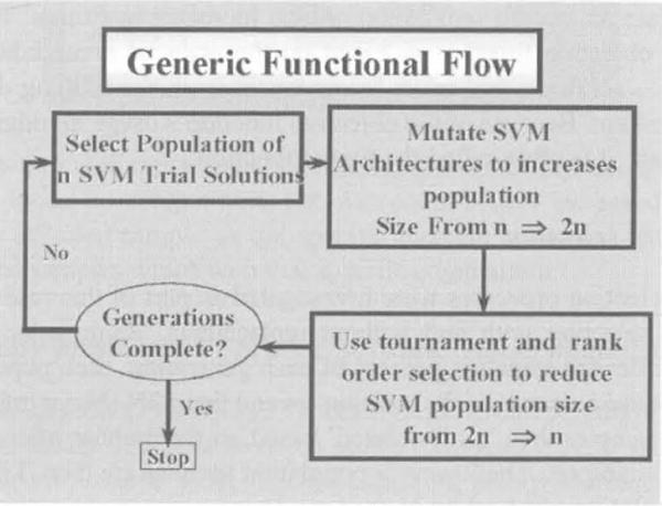
Generic description of Evolutionary Programming derived families of Support Vector Machines (see online version for colours)

The mutation and selection cycle is repeated for a pre-specified number of generations. If this cycle results in population elements (candidate solutions) that increase in fitness, the average and maximum population fitness will asymptotically increase to some maximum value as the population is evolved over several generations.

The mutation process implemented in this study uses a self-adaptive mutation vector. This vector stores the variances corresponding to the normal distribution being sampled for each configurable parameter. During mutation, each element of the mutation vector is updated using the following expression:

$$v_i^{\prime }=v_i{e}^{\left(\frac{1}{\sqrt{2n}}\mathrm{N}(0,1)+\frac{1}{\sqrt{2\sqrt{n}}}{\mathrm{N}}_i(0,1)\right)}$$ (1)

where n is the total number of configurable parameters being evolved. (Note, here n is not the population size, it is the length of the v vector for each element of the population.) N(0, 1) is a standard normal random variable sampled once for all n parameters of the v vector. N_i(0, 1) is a standard normal random variable sampled for each of the n parameters in the v vector.

The second step of this more rigorous mutation process comprises the updating of each configurable parameter for all elements of the evolving population. If we let the vector x_i denote these elements for each of the individual member of the population, this update process will be accomplished as follows:

$$x_i^{\prime }=x_i+C{v}_i^{\prime }$$ (2)

where i is the ith component of the x vector. x is the vector containing the current values of the configurable parameters, v′_i is the variance computed by Equation (1) and C is a standard Cauchy random variable (this random variable has slightly longer tails than a normal random variable and usually offers slightly better mutation performance). This new x′_i vector is then computed, in turn, for each child element of the next generation.

While one anticipates that the mutation process will improve the fitness of individual population elements, the objective function is used to sort out which elements to keep and which to discard. As such, the objective function chosen affects the ability of the EP process to generate an overall population, which increases in fitness. Typically (and in this study), this objective function is based on the error of a candidate solution over the training data – solutions that make fewer mistakes on the training data are declared ‘more fit’ and are kept. Because of the objective function’s usage in judging the fitness of candidate solutions, it is often called the fitness function.

2.2 Tournament selection

Three types of selection processes were investigated as part of this research: rank order, and tournament selection with and without replacement. Rank order selection is the simplest, where after the mutation process of each generation, each population sample is evaluated against the elements of the training set and these 2N (N = number of samples in the training set) samples then ‘rank ordered’ based on the number of correctly classified samples of the training set. The lowest N population samples are then ‘killed off’, thereby reducing the population size back to N.

Tournament selection (with and without replacement) is a bit more complex, where selection without replacement is depicted in Figure 2. The advantage of this approach is that the population elements undergo more competitions, thereby allowing samples with initially low fitness to improve and, consequently, not be eliminated early, which could occur with a simpler process, such as rank order selection. The process operates as follows. Each of the 2N population elements is deterministically selected, say $\mathcal{E}$, (see Figure 2) as a candidate sample.

Figure 2.

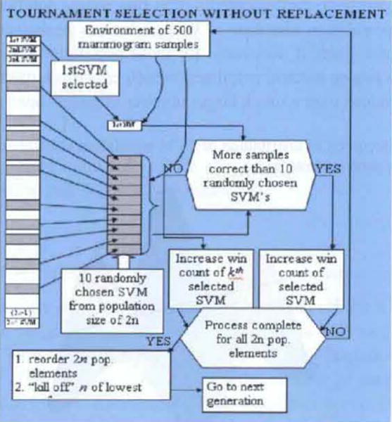
Tournament selection without replacement (see online version for colours)

Then $\mathcal{F}$ samples (usually $\mathcal{F}=10$) are randomly selected, which are competed against the first deterministically selected sample. If the $\mathcal{E}$ sample wins the competition (classifies the most samples in the training set correctly) then $\mathcal{E}$ keeps its place in the 2N array of samples and its ‘win count’ is increased. If $\mathcal{E}$ looses, then the win count of randomly selected $\mathcal{F}$ sample subset’s win count is increased. This same process is repeated for each of the 2N samples and the resultant population set is reordered based on the number of win counts, with the lower ranking N population elements then being ‘killed off’, thereby reducing the population size again to N.

Tournament selection with replacement operates in the same way, except the samples are replaced if they loose the competition. The win count is also increased for either the $\mathcal{E}$ deterministically selected sample or the specific element belonging to the $\mathcal{F}$ subset of randomly selected samples which won that specific competition.

2.3 Evolutionary programming process provides global minimum

This section describes the methodology by which the software paradigm is developed for implementing the family of SVMs so that a global minimum may be realised. This is an important component because SVM statistical learning theory addresses the problem of how a global minimum is theoretically possible by minimising the true risk as opposed to the empirical risk. The reader will recall that training neural networks by back propagation, using the gradient method, almost always results in a local minimum, as only the empirical risk is minimised.

A great majority of the kernels utilised in SVM classification problems involve one parameter, which has to be optimised (i.e., the σ for the Gaussian or exponential function, or the order of the spline or polynomial). The other is the regularisation parameter, C, which specifies the upper bound on the size of the Langrangian multipliers. A second parameter may sometimes be required for some kernels, such as the hyperbolic tangent. Consequently, the search (or solution) space can generally be specified by a two (or three) dimensional search apace, where one axis specifies the bounds on the regularisation parameter while the other axis specifies the parameter characterising the mapping kernel K(x_i, x_j) = ϕ(x_i)•ϕ(x_j). For example, in the Figure 3, one axis could represent the kernel parameter, the other axis the regularisation parameter while the 3rd axis could represent the area under the receiver operator characteristic curve (AZ) index. It is clear that if the grid is partitioned into grids of small size, some of these elements will be over or at least close to the global minima. However, a more dense SVM distribution will require a large population size, which will result in a longer solution time. Consequently, we have implemented a dual fine/course solution approach, where a large initial set of population elements is used, which is optimised over only a small number of generations. Then, if necessary, for those population samples in the region of the global minima, a coarse method is utilised, which contains a much smaller population size, but can be optimised over a much larger number of generations in less time.

Figure 3.

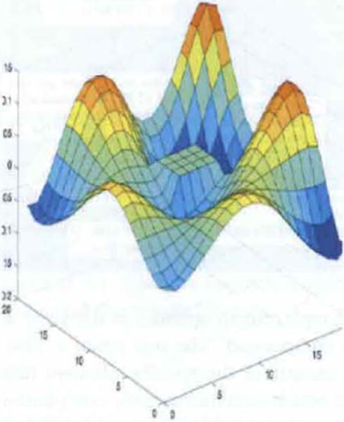
Generic description of distribution of SVM population elements over solution space (see online version for colours)

2.4 Support vector machines

We now summarise SVMs (Cristianini and Shawe-Taylor, 2000; Gunn, 1998; Burges, 1998). This discussion provides the theoretical explanation for why SVMs can always be trained to a global minimum, and thereby should provide better diagnostic accuracy, when compared with neural network performance trained by back propagation. Assume there exist N observations from a data set. Each observation (or training example) consists of a vector x_i containing the input pattern and a corresponding known classification yi. The objective of the learning machine is to formulate a mapping x_j → y_j Now consider a set of functions f(x, α) with adjustable parameters a, that defines a set of possible mappings x → f(x, α). Here, x is given and α is chosen. In the case of a traditional neural network of fixed architecture, the α values would correspond to the weights and biases. The quantity R(α), known as the expected (or true) risk, associated with learning machines is defined as:

$$R(\alpha )={\displaystyle \int \frac{1}{2}\left|y-f(\mathbf{x},\alpha )\right|}p(\mathbf{x},y)d\mathbf{x}dy$$ (3)

where, p(x, y) is an unknown probability density function from which the examples were drawn. This risk function is the expected (or true) value of the test (or validation) error for a trained learning machine. It may be shown that the best possible generalisation ability of a learning machine is achieved by minimising R(α), the expected (or true) risk. This generalisation bound, for binary classification, holds with the probability of at least 1 − η (0 ≤ η ≤ 1) for all approximating functions that minimise the expected (or true) risk.

$$R(\alpha )\le R_{\text{emp}}(\alpha )+\sqrt{\left(\frac{h\left(\log \left(\frac{2N}{h}\right)+1\right)-\log \left(\frac{\eta }{4}\right)}{4}\right)}.$$ (4)

The first term on the right hand side of the above equation is known as the ‘empirical risk’, where the empirical risk R_emp(α) is expressed by:

$$R_{\text{emp}}(\alpha )=\frac{1}{2N}{\displaystyle \sum _{i=1}^N\left|y_i-f({\mathbf{x}}_i,\alpha )\right|}.$$ (5)

This function is a measure of the error rate for the training set for a fixed, finite number of observations. This value is fixed for a particular choice of α and a given training set (x_i,y_i). The second term in the above expression is the “Vapnik-Chervonenkis (VC) confidence interval”. This term is a function of the number of training samples N, the probability value η and the VC dimension h. The VC dimension is the maximum number of training samples that can be learned by a learning machine without error for all possible labelling of the classification functions f(x, α), and is, therefore, a measure of the capacity of the learning machine. In traditional neural network implementations, the confidence interval is fixed by choosing a network architecture a priori. The function is minimised by generally obtaining a local minimum from minimising the empirical risk through adjustment of weights and biases. Consequently, neural networks are trained based on the Empirical Risk Minimisation (ERM) principle. In a SVM design and implementation, not only is the empirical risk minimised, the VC confidence interval is also minimised by using the principles of Structural Risk Minimisation (SRM). Therefore, SVM implementations simultaneously minimise the empirical risk as well as the risk associated with the VC confidence interval, as defined in the above expression. The above expression also shows that as N → ∞, the empirical risk approaches the true risk because the VC confidence interval risk approaches zero. The reader may recall that obtaining larger and larger sets of valid training data would sometimes produce (with a great deal of training experience) a better performing neural network using classical training methods. This restriction is not incumbent on the SRM principle and is the fundamental difference between training neural networks and training SVMs. Finally, because SVMs minimise the true risk, they provide a global minimum.

2.5 Kernel functions and similarity

Consider now kernel functions and their application to SVMs. SVM solutions in nonlinear, non separable learning environments, utilise kernel based learning methods. Consequently, it is important to understand the practical implications of using these kernels. Kernel based learning methods use a kernel as a nonlinear similarity to perform comparisons. That is, these kernel mappings are used to construct a decision surface that is nonlinear in the input space, but has a linear image in the feature space. To be a valid mapping, these inner product kernels must be symmetric and also satisfy Mercer’s theorem (Cristianini and Shawe-Taylor, 2000). The concepts described here are not limited to SVMs, and the general principles also apply to other kernel based classifiers as well.

A kernel function should yield a higher output from input vectors which are very similar than from input vectors which are less similar. An ideal kernel would provide an exact mapping from the input space to a feature space, which was a precise separable model of the two input classes; however, such a model is usually unobtainable, particularly for complex, real-world problems, and those problems in which the input vector provided contains only a subset of the information content needed to make the classes completely separable. As such, a number of statistically-based kernel functions have been developed, each providing a mapping into a generic feature space that provides a reasonable approximation to the true feature space for a wide variety of problem domains. The kernel function that best represents the true similarity between the input vectors will yield the best results, and kernel functions that poorly discriminate between similar and dissimilar input vectors will yield poor results. As such, intelligent kernel selection requires at least a basic understanding of the source data and the ways different kernels will interpret that data.

Some of the more popular kernel functions are the (linear) dot product, the Gaussian Radial Basis Function (GRBF), the Exponential Radial Basis Function (ERBF), and the polynomial kernel, which will be discussed below. However, specific kernels can be constructed using attributes from the feature space. That is, the kernel is developed by beginning with the features and then formulating the inner product. An advantage of this approach is that there is no need to check for the positive semi-definiteness because it follows automatically from the definition of the inner product (Cristianini and Shawe-Taylor, 2000).

The dot product and polynomial kernels are given by:

$$K(\mathbf{\mu },\mathbf{v})=\mathbf{\mu }•\mathbf{v}=\Vert \mathbf{\mu }\Vert \Vert \mathbf{v}\Vert \cos \theta$$ (6)

and

$$K(\mathbf{\mu },\mathbf{v})={(\mathbf{\mu }•\mathbf{v}+1)}^d$$ (7)

respectively, where u. are v, two arbitrary input vectors as defined above. Both use the dot product (and therefore the angle between the vectors) to express similarity; however, the input vectors to the polynomial kernel must be normalised (i.e., unit vectors). This restricts the range of the dot product to ±1, yielding kernel outputs between 0 and 2^d, where d is the degree of the polynomial. The implication of the dot product kernel having a positive and negative range (vs. the strictly non-negative polynomial kernel) is that the classification process can learn from the unknown vector’s dissimilarity to a known sample, rather than just its similarity. While the dot product kernel will give relatively equal consideration to similar and dissimilar input vectors, the polynomial kernel will give exponentially greater consideration to those cases which are very similar than those that are orthogonal or dissimilar. The value of d determines the relative importance given to the more similar cases, with higher values implying a greater importance. Measures of similarity for these two kernels are depicted in Figures 4 and 5.

Figure 4.

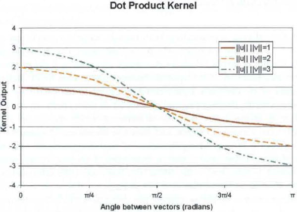
Dot product kernel output as function of angle (see online version for colours)

Figure 5.

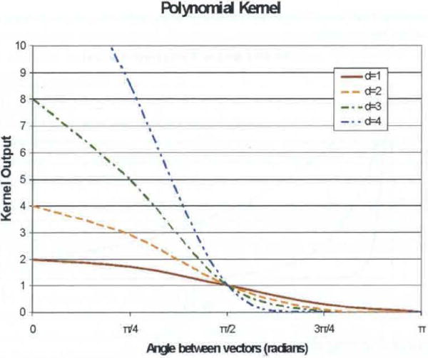
Polynomial kernel output as function of angle between input vectors (see online version for colours)

The GRBF and ERBF kernels use the Euclidean distance between the two input vectors as a measure of similarity instead of the angle between them (see Figure 6).

$$\mathit{\text{Gaussian}}\{K(\mathbf{\mu },\mathbf{v})\}=\mathit{\text{exp}}\left(-\frac{{\Vert \mathbf{\mu }-\mathbf{v}\Vert }^2}{2{\sigma }^2}\right).$$ (8)

$$\mathit{\text{Exponential}}\{K(\mathbf{\mu },\mathbf{v})\}=\mathit{\text{exp}}\left(-\frac{{\Vert \mathbf{\mu }-\mathbf{v}\Vert }^2}{2{\sigma }^2}\right).$$

Since ∥ μ − v∥ is always non-negative, both kernels achieve a maximum output of one when ∥ μ − v∥ = 0, and approach zero as ∥ μ − v∥ increases. This approach is made faster or slower by smaller or larger values for σ, respectively. Figure 6 shows the output of the GRBF kernel as a function of the squared distance between the input vectors for several different values of σ. The same figure could demonstrate the ERBF by relabelling the horizontal axis with the distance (instead of squared distance) between the input vectors.

Figure 6.

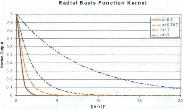
Gaussian RBF kernel output as function of squared distance between vectors (see online version for colours)

It is clear from the figure that the distance at which the kernel output reaches approximately zero varies with sigma, and therefore the choice of sigma for this kernel is essential in properly distinguishing the level of similarity between two input vectors. If the value of sigma is too small – that is, most pairs of vectors are far enough apart that the kernel output is near zero – the SVM will have too little information to make an accurate classification. If the value of σ is too large, so that even very distant pairs of input vectors produce a moderate output, the decision surface will be overly smooth. This may mask smaller distinctive characteristics that exist in the ideal decision surface, and will also increase the effect of outliers in the training data have on the classification of an unknown point.

2.6 Statistical learning theory/decision methods

Beginning with the example of least squares, this section will now address essential decision learning theory concepts necessary for these applications, which are:

• Data items are embedded into a vector space called a feature space.

• Ascertaining linear relations developed from the data items in a feature space.

• Using kernels in an attempt to design and implement algorithms so that the coordinates of the imbedded points are not directly used. Only the pair wise inner products of these are used.

• From the above item, the pair wise inner products can be computed efficiently using a kernel function directly from the original data items.

In this work, new decision paradigms are proposed for use in clinical applications. It is imperative to show exactly why these methods are preferable to existing techniques. The natural way to show this is by taking a comparative look the mathematical foundations for the various decision methodologies. This is provided below as evidence that the proposed methods will generalise and are scalable.

The reader should also consult reference (Shawe-Taylor and Cristianini, 2004) for a comprehensive discussion of statistical learning theory. For example, Shawe-Taylor and Cristianini (2004), describes: the theory of kernel functions, how statistical stability can be controlled, develops tools for analysing data in a kernel-defined feature space, creates a novelty detection algorithm, studies discovering patters using eigen-analysis, and develops a number of approaches for creating kernels.

2.7 Overview of the decision methods

• Linear regression may be used when linear relations between the input variables and the output decision are assumed. However, the relationship may not be linear and the solution may not be exact, which presents as a competing compromise when determining the solution.

• Principal Component Analysis (PCA) may be introduced to the linear problem discussed above, which has the desirable effect of reducing the dimensionality of the data set but does not address the possibility of non-linear relationships. PLS may also be used to reduce the dimensionality with some advantages over PCA in that it represents an intelligent learning system.

• A nonlinear mapping may be found that transforms the original problem into the linear-type problem discussed above. This relies on determining the proper kernel that allows the data transformation. Once this is found, the PLS may be applied, which gives the KPLS approach (kernel-PLS).

• The SVM development is provided because it is better known for its ability in achieving a global minimum in training, whereas KPLS’s ability to achieve this is less known but theoretically possible. The ability to train the KPLS in near real time (for data bases of reasonable size) is a significant main advantage over the SVMs, trained by gradient methods. Thus, the K-PLS represents the new decision method and the SVM is used solely as a means of comparison as well as is the neural network.

2.8 Primal Linear Regression (PLR)

The objective of PLR is the standard problem of finding a function for where the differences between training pairs are small. This will be accomplished by the most commonly chosen measure of ‘collective’ discrepancy (sum) between the training data (the reader will note that this regression analysis is formulated as a learning problem) and a particular function, g, and is represented by:

$$\pounds (\mathrm{g},\mathrm{S})=\pounds (\mathbf{w},\mathrm{S})={\displaystyle \sum {\{{\mathrm{y}}_{\mathrm{i}}-\mathrm{g}({\mathbf{x}}_{\mathbf{i}})\}}^2={\displaystyle \sum {\left|{\mathbf{\xi }}_{\mathbf{i}}\right|}^2={\displaystyle \sum \pounds \{({\mathbf{x}}_{\mathbf{i}},{\mathrm{y}}_{\mathrm{i}}),\mathrm{g}\}}}}.$$ (9)

Observe that £{(x_j,y_j),g} = |ξ_i|² (which is the same notation) both represent the squared loss error of g on the sample (x_i, y_i) and £(f, S) denotes the collective loss of a function f on the training set S. One can define the regression learning problem with this simple formulation: The learning problem is that of identifying a vector w ⊂ ℑ, which minimises the collective loss.

This problem was originally studied by Gauss and is commonly known as least squares approximation. The collective loss is minimised by finding w such that the collective loss is minimised as shown below. First, define ξ = [y−Xw]. Note that X is defined as the matrix whose rows are the row vectors, X = {x₁, x₂^T, x₃^T,………. x₁^T} and y denotes the vector y = {y₁, y₂, y₃…y₁}. Note that, the Equation (9) expression is related to this linear problem by letting the g = {g₁, g₂, g₃…g₁} with g = Xw.

The loss is given by: Loss = £ (w, S) = |ξ| = [y − Xw ] ^T [y − Xw], where T is the transpose of the vector difference. To find the correct w, form:

$$\partial \pounds (\mathbf{w},\mathrm{S})/\partial \text{w}=-2{\mathbf{X}}^{\mathbf{T}}\mathbf{y}+2{\mathbf{X}}^{\mathbf{T}}\mathbf{X}\mathbf{w}=0$$ (10)

which becomes: (X^TX)w = X^Ty. Solving for w gives, w = (X^TX)⁻¹ X^TY. Although Equation (10) has the same form as the standard least squares approximation, there is a fundamental difference in the formulism. In the standard least squares approach, the form of w is normally assumed and then the system is minimised with respect to this assumed functional relation in contrast to finding the unique w = w_CL that minimises the collective loss, which is the intent here. That is, many least squares solutions exist that satisfy equation (10). However, only one solution, g = g(x, w_CL), exists that will minimise the collective loss, which is characterised by the vector w_CL.

If (X^TX)⁻¹ is singular (meaning there is not enough data to ensure that (X^TX)⁻¹ is invertible), a pseudo inverse is used to solve the problem. This pseudo inverse will ascertain w, which satisfies (X^T X)w = X^Ty, with a minimum norm. Alternately, one can trade- off the size of the norm against the loss, which is the process known as ridge regression. That is, ridge regression corresponds to solving the optimisation problem: Min £(w, S) = min λ |w|² + Σ[y_i − g(x_i)]², where λ = the positive number, which establishes the trade off between the norm and loss and, consequently, controls the degree of regularisation. Ridge regression is further discussed in Cristianini and Shawe-Taylor (2000).

2.9 Non-linear mappings

The methods presented thus far primarily addressed the problem of identification of linear relationships between an output and features characterised by the expressions x_i. However, most practical problems can only be estimated as a nonlinear mapping from the x_i into the y_i. This mapping leads to the definition of a kernel function (ℑ), which is: A kernel function is one that for all x, z ε X, satisfies

$$\Im (\mathbf{x}\mathbf{,}\mathbf{z})=\langle \mathrm{\varphi }(\mathbf{x}),\mathrm{\varphi }(\mathbf{z})\rangle ,$$ (11)

where ϕ is a mapping from and input into a feature space F, defined as:

$$\mathrm{\varphi }:\mathbf{X}\Rightarrow \mathrm{\varphi }(\mathbf{X})\in \mathrm{F}.$$ (12)

More will be said about kernel defined feature space subsequently.

2.10 Kernel principal component analysis (K-PCA)

PCA is used to reduce the effective dimensionality of a data set, which causes the representation (of the information content in the data) to lie on a lower dimensional surface. This well known fact is very useful in the solution of practical problems because fewer input variables are needed to characterise the data. Consequently, one can then re-construct the data from a ‘new’ set of coordinates. For a linear system, the problem is equivalent to projecting data onto a smaller dimensional linear subspace so that the distance between the vector and its projection is minimised. Minimising the average squared distance between the vectors and their projections is equivalent to projecting data onto a subspace spanned by the first k eigenvectors of the X^TX matrix, given by: X^TXv_I = λ_iv_i. Consequently, the coordinates of a new vector X in this new space is obtained from its projection onto the eigenvector (X, v_c) with c = 1, 2, 3…, k.

The more complex problem of adapting this PCA approach to a non-linear system is considered now, which is provided by a mapping. This mapping is accomplished by first embedding the data into a feature space. Kernels are used to define the feature space, since an algorithm can be rewritten using a format, which requires only inner products between the inputs. Therefore, non-linear relationships between data variables may be found by embedding this data into the kernel-induced feature space, where linear relations can be found by means of PCA. This approach has come to be known as kernel PCA.

2.10.1 Partial Least Squares (PLS) regression

PLS is another method that reduces the number of variables needed to optimally characterise the environment. PLS has one major advantage when compared to PCA and that is both independent and dependent variables are used in the compression step. Adding this dependent variable usually has a profound effect on the PLS predictive performance when compared to PCA. Secondly, because the independent variables are compressed in such a way to achieve an apriori specified output, PLS can be characterised as a supervised leaning process, and, therefore, defined as an intelligent process. The collective result of these advantages is that an intelligent linear training method results, which runs in real time (for data sets of reasonable size), and whose results (Land et al., 2005a, 2005b) have been shown to agree with statistical learning theory paradigms that theoretically have been demonstrated to provide global minima.

PLS was originally introduced by these researchers (Wold, 1975; Wold et al., 2001) who were motivated by finding a practical solution to data analytic problems in econometrics and the social sciences. The same fundamental problem is addressed as that for PCA: to fit a calibration model to empirical data, and then use this model to predict certain outputs, given a set of sparse data, not ordinarily large enough to characterise all the environment variables (i.e., an undetermined system where an undetermined system would result when using primal linear regression). Therefore, PLS can be viewed as a better Principal Components Analysis (PCA). In PLS data are first transformed into a different and non-orthogonal basis, similar to Principal Component Analysis (PCA), and only a few (the most important) PLS components (or latent variables) are considered for building a regression model (just as in PCA). The difference between PLS and PCA is that the new set of basis vectors (similar to the eigenvectors of X^TX in PCA) is not a set of successive orthogonal directions that explain the largest variance in the data, but are actually a set of conjugant gradient vectors to the correlation matrices that span a Krylov space (Ipsen and Meyer, 1998; Awais, 2007). Just like in PCA, the basis vectors can be peeled off from the data matrix X successively in the NIPALS algorithm (Nonlinear Iterative PLS), also introduced by Wold (1996) by approximating X as X = TP^T (similar to X = TB in PCA, where the T contains the scores and B is a matrix of eigenvectors corresponding to the largest eigenvalues for X^TX).

PLS is sometimes called abstract factor analysis, or rank reduction, because physically significant quantities comprising (and within) the system cannot always be identified directly by using the mathematical modelling process (Malinowski, 1977). However, the factor analysis method of PLS can be of significant help in identifying key environment factors in the data, which can be extracted from the environment, and used by the PLS modelling process. Furthermore, PLS is a ‘full spectrum approach’, which means that efficient outlier techniques can be used by identifying residuals resulting from the PLS process. These outliers are those environment samples which are “out of the nominal range”, and therefore not representative of valid training samples. The practical consequence of using this capability means that these methods may be employed to ‘clean’ the data sets of those contradictory samples that can degrade CAD classification and diagnostic performance. Consequently, estimated output can also be carefully examined to ascertain if these techniques should be used (Martens and Naes, 1989; Haaland and Thomas, 1988). The authors are not aware that comparable techniques exist for the standard multilayer feed forward neural network, trained by back propagation.

2.10.2 Kernel defined feature space

Kernel defined feature mappings are discussed next. Previously, it was stated that non-linear relationships between data variables may be found by embedding this data into a kernel induced feature space. This kernel ‘trick’ is used in PLS resulting in K-PLS. That is, consider now the following embedding map: ϕ : X ∈ ℜⁿ ⇒ ϕ (X) ε F ⊆ ℜ^N The objective of the map is to convert the non-linear relations into linear ones. This map will therefore reflect the expectations regarding the relation y= g(X), which must be learned. That is, the mapping will ‘recode’ the data set S as: S = {ϕ((x₁), y₁), ϕ((x₂), y₂), ϕ((x₁), y₁)}. This mapping of the data set is from nonlinear input space to a linear feature space. That is, the environment data representation in the input X space is non-linear. However, after the x_i data are processed by the ϕ((x_i), y_i) function, the data characterised by this mapping is linear, with the happy result that linear techniques may be used on the mapped data while preserving the non-linear properties represented in the input space. This mapping is accomplished, as previously stated, by using a valid kernel function.

In summary, the purpose of this kernel function is to map the data into a feature space where the original non linear pattern (or environment) now appears as linear. The practical consequence is that linear techniques may be applied to the feature space data without in any way disturbing the nonlinear environment properties in the input space. Adding this kernel induced capability to the PLS approach already described means that a real time, non-linear optimal training intelligent method now exists, which can be used to perform CAD diagnosis. A second advantage of this approach is that the Kernel computes inner products in the feature space directly from inputs.

3 Data set descriptions

Two data sets, described below, were used to evaluate these new EP/ES Statistic SVM learning system and the K-PLS machine intelligence paradigms.

3.1 Magnetic resonance mammography data set

The Magnetic Resonance Mammography (MRM) data set consisted of 395 samples, approximately equality divided between cases and controls. All cancer-positive cases were pathology verified. The patient population represents a subset of those patients encountered in diagnostic mammography that are undergoing diagnostic MRM. The data is retrospective and therefore was acquired with no specific imaging protocol. This collection of MRM subjects are patients who

• have a known diagnosis of cancer (to determine extent of disease, evaluate for synchronous lesions)

• have equivocal mammogram (suspicious mammogram) finding but not clearly localised

• require follow-up after therapy (for example, dense breasts in an XRT/lumpectomy patient).

The collection also consists of patients that were scanned prior to their surgeries (known cancer positive patients). The cases that have an equivocal mammogram are usually benign and are followed by repeat MRM, ultrasound, or x-ray mammogram. If an equivocal finding looks suspicious, it is biopsied. The patient data used as input features for the Logistic Regression (LR) modelling may be divided into two categories (I) non-image type (NI), and (II) and image type (IM) features observable in the MRM image. The NI features were

• patient age

• race/ethnicity

• weight

• age of menarche

• duration of menstruation

• age of menopause

• number of full term deliveries

• duration of hormone replacement therapy

• family history of breast cancer (yes or no)

• cigarette smoking (yes or no).

The IM based features were lesion

• size

• shape

• margin.

Since MRM requires contrast injection, the lesion description is dependent upon its enhancement. The shape and margins for masses are normally assessed from the first post-contrast image to avoid washout or enhancement (Morris and Liberman, 2005). The database was pared-down by discarding subjects for a particular trial that had open features fields for a given model arraignment (for either feature non-applicable reasons or when the feature was not-available).

3.2 BI-RADS and clinical feature data set

The other data set contains BI-RADS features in addition to the halo, family history and age features and comprises cases from women with biopsy verified malignant masses, and the controls are women with benign breast lesions. For this work breast masses define the lesion and the presence of calcifications, singular or clustered, are excluded. The benign controls consist of two distinct classes: those masses determined benign by biopsy and those determined benign after two-years follow-up without biopsy. The study consists of 175 distinct individuals with 55 malignant cases, 40 benign controls determined by biopsy, and 80 benign follow-up controls without biopsy. The data were collected from the diagnostic center at the Moffitt Cancer Center & Research Institute.

The standard BI-RADS descriptors used as input features are mass shape, mass margin, overall breast, composition, and density. In addition to the BI-RADS derived features, the presence of a halo (yes or no) around the tumour, family history (yes or no), and age were also used as input features. For reference, the relevant BI-RADS descriptions are provided. Mass shape is a five-category rating: round, oval, lobulated, irregular, and architectural distortion. Mass margin is a five-category rating: circumscribed-well defined, microlobulated, indistinct, obscured, speculated. Density is a four-category rating in the vicinity of the mass relative to the surrounding area: high, low, equal, or fat-containing-radiolucent. Overall breast composition is a four-category rating: entirely fat, scattered fibrogaldular tissue, heterogeneously dense, and extremely dense.

4 Results

This section focuses on three topics:

• performance comparison of the EP/ES SVM stochastic hybrid with the standard iterative method of training using an identical data set and statistical cross validation methods

• performance tradeoff and diagnostic accuracy of the auto-K-PLS, K-PLS and the EP/ES SVM hybrids using the MRM and non-image data sets

• EP/ES SVM hybrid and K-PLS classification accuracies using the BI-RADS and clinical feature data set.

4.1 Performance comparison between iteratively derived and EP derived SVMs

Performance comparison for the iterative and EP derived SVM approaches (using the above described mutation method) are depicted in Figures 9 and 10. Both the same as well as different kernels were evaluated by both methods. However, the EP SVM results used tournament selection with replacement. As expected, the results are essentially the same for identical kernels, the same data set, and the same statistical cross validation methods. For example, for the s2000, GRBF, and dot product kernels, the EP SVM approach obtained very small percentage performance improvements of 0.22, 0.76 and 0.0%, respectively, when compared to those obtained by the iteratively trained method. These results demonstrated, however, that the two methods yield essentially the same result. Secondly, both methods produced essentially perfect classification results, generally ranging from 0.926 to 0.931. Only the hyperbolic tangent kernel yielded a less accurate result of 0.87. These were also expected results because all ambiguous findings were ‘scrubbed’ from the features describing the screen film data set.

Figure 9.

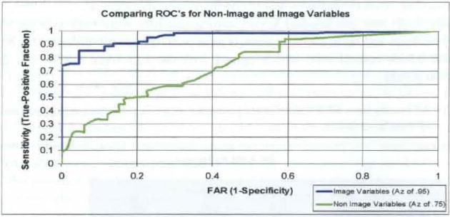
Comparing non-image and image ROC curves (see online version for colours)

Figure 10.

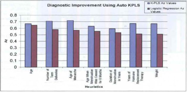
Predictive improvement gained with auto K-PLS in comparison with logistic regression (see online version for colours)

Finally, both sum and product kernel implementations were built into the EP SVM software package and these multiple kernels gave five fold cross validation AZ indices of 0.925 and 0.926, respectively, which agreed with the individual GRBF and degree-2 polynomial results.

4.2 Comparison of the Auto K-PLS, K-PLS and Stochastic EP/ES SVM using the MRM data set for image and non-image features

Both Non-Image (NI) and image (IM) type features were evaluated relative to their contribution to diagnostic accuracy (see data section for description). Table 1 depicts results for two types of K-PLS paradigms: auto-K-PLS and K-PLS. Auto K-PLS is an automated process which finds the optimal sigma value for the Gaussian Radial Basis Function (GRBF) mapping kernel as well as eliminating the outliers by an automated process. K-PLS has neither of these features. The EP-SVM process employs the same GRBF mapping kernel and used the EP process to optimise both the sigma (σ) value and regularisation parameter(C). Both auto-K-PLS and K-PLS result in essentially the same ROC AZ value (average of 0.76), while the EP-EVM result of 0.64 is 18.7% lower. This difference is attributed to the inclusion of the data set ‘outliers’. The MRM Image features size, shape and margin yielded a much better K-PLS AZ result, as expected, of 0.96. The EP-SVM process produced and expected lower AZ of 0.91, again because of the outliers. These ROC AZ curves are depicted in Figure 9.

Table 1.

AZ results for non-Image (NI) and image (IM) data sets.

Data set	Auto K-PLS AZ	KPLS AZ	EP-SVM AZ
NI	0.77	0.75	0.643052
IM	0.962742	0.9549	0.906607

Finally, Figure 10 demonstrates the K-PLS diagnostic performance improvement for some of the more significant non-image features, when compared to the LR diagnostic process (Land et al., 2006) for the development of the LR results). Note that in all cases a significant amount of diagnostic information in contained in the non-linear mapping region of the features to the diagnostic result. This is an important new finding, and demonstrates the importance of collecting and using this clinical information in the diagnostic process. Moreover, it shows that the choice of decision methodology is as important as determining input features with predictive capabilities, which is clearly demonstrated in Figure 10.

4.3 EP/ES Stochastic SVM and K-PLS results using BI-RADS, Halo and clinical feature variables

Table 2 shows the results using three EP/ES selection methods, where each selection method uses eight different mapping kernels and five fold cross validation for the full complement of BI-RADS, Halo, family history, and age features. Results are shown for all five folds as well as the average across all five folds The data in this table demonstrate that all kernels and selection methods yield approximately the same AZ results of approximately 0.90–0.92, which are excellent diagnostic/classification performances. K-PLS results, shown in Table 3, of AZ ~ 0.91 agrees well with the EP/ES stochastic SVM results and could most probably be improved by examining other mapping kernels.

Table 2.

EP/ES Stochastic SVM results with different kernels, and different selection methods using all feature variables

SVM
Selection method	Kernel	Fold1	fold2	fold3	fold4	fold5	avgAz
Rank	Add	0.869318	0.867754	0.956522	0.93939	0.9359	0.91378
Rank	Dot	0.871212	0.891304	0.929348	0.95455	0.95727	0.92074
Rank	Mult	0.856061	0.862319	0.960145	0.94318	0.93162	0.91067
Rank	Poly	0.857955	0.875	0.95471	0.93939	0.90598	0.90661
Rank	Rbf	0.856061	0.887681	0.949275	0.94697	0.95727	0.91945
Rank	S2000	0.867424	0.891304	0.929348	0.95076	0.95299	0.91837
Rank	spline	0.867424	0.862319	0.927536	0.94318	0.93162	0.90642
Rank	Tanh	0.869318	0.894928	0.938406	0.95076	0.92308	0.9153
Tourn w/o Repl	Add	0.869318	0.867754	0.956522	0.93939	0.9359	0.91378
Tourn w/o Repl	Dot	0.875	0.887681	0.92029	0.95455	0.94444	0.91639
Tourn w/o Repl	Mult	0.86553	0.869565	0.956522	0.94318	0.9188	0.91072
Tourn w/o Repl	Poly	0.863636	0.876812	0.956522	0.94318	0.90171	0.90837
Tourn w/o Repl	Rbf	0.856061	0.887681	0.949275	0.94697	0.95727	0.91945
Tourn w/o Repl	s2000	0.886364	0.880435	0.934783	0.95833	0.97009	0.926
Tourn w/o Repl	spline	0.867424	0.862319	0.927536	0.94318	0.93162	0.90642
Tourn w/o Repl	Tanh	0.875	0.891304	0.938406	0.95076	0.93162	0.91742
Tourn w/Repl	Add	0.876894	0.873188	0.956522	0.93939	0.92308	0.91382
Tourn w/Repl	Dot	0.875	0.887681	0.92029	0.95455	0.94444	0.91639
Tourn w/Repl	Mult	0.856061	0.862319	0.960145	0.94318	0.93162	0.91067
Tourn w/Repl	Poly	0.863636	0.876812	0.956522	0.94318	0.90171	0.90837
Tourn w/Repl	Rbf	0.878788	0.876812	0.923913	0.94697	0.92735	0.91077
Tourn w/Repl	s2000	0.852273	0.891304	0.929348	0.94318	0.98718	0.92066
Tourn w/Repl	spline	0.878788	0.865942	0.927536	0.94318	0.93162	0.90941
Tourn w/Repl	Tanh	0.875	0.884058	0.938406	0.94697	0.92735	0.91436

Table 3.

K-PLS results using a Gaussian kernel with five latent variables

KPLS options:	Outliers	Latent variables	Sigma	Az
	No	5	4.792	0.906894

The question now becomes: which variables are the most significant contributors to diagnostic/classification accuracy. Several LR statistical studies were done, as described in Land et al. (2006) and not reported here, to ascertain the most important features in this data set. This research showed that Halo, Family History and Breast composition were not contributors to the diagnostic/classification accuracy. Consequently, these features were removed from the original dataset and the remaining subset was processed by all of the same EP/ES Stochastic SVM and K-PLS classifiers. The results are depicted in Tables 4 and 5.

Table 4.

EP/ES Stochastic SVM results with different kernels, and different selection methods using a selected subset of feature variables

SVM
Selection method	Kernel	fold1	fold2	fold3	fold4	fold5	avgAz
Rank	Add	0.818182	0.884058	0.949275	0.94697	0.97009	0.91371
Rank	Dot	0.867424	0.884058	0.945652	0.95076	0.98718	0.92701
Rank	Mult	0.818182	0.876812	0.952899	0.93939	0.97436	0.91233
Rank	Poly	0.814394	0.891304	0.949275	0.95076	0.97009	0.91516
Rank	Rbf	0.882576	0.880435	0.949275	0.95076	0.97436	0.92748
Rank	s2000	0.867424	0.887681	0.945652	0.95076	0.98291	0.92688
Rank	Spline	0.876894	0.873188	0.945652	0.94697	0.98718	0.92598
Rank	Tanh	0.867424	0.916667	0.949275	0.95833	0.95727	0.92979
Tourn w/o Repl	Add	0.82197	0.876812	0.952899	0.94318	0.97222	0.91342
Tourn w/o Repl	Dot	0.867424	0.884058	0.945652	0.95076	0.98718	0.92701
Tourn w/o Repl	Mult	0.818182	0.876812	0.952899	0.93939	0.97436	0.91233
Tourn w/o Repl	Poly	0.814394	0.891304	0.949275	0.95076	0.97009	0.91516
Tourn w/o Repl	Rbf	0.882576	0.880435	0.949275	0.95076	0.97436	0.92748
Tourn w/o Repl	s2000	0.867424	0.887681	0.945652	0.95076	0.98291	0.92688
Tourn w/o Repl	Spline	0.876894	0.873188	0.945652	0.94697	0.98718	0.92598
Tourn w/o Repl	Tanh	0.867424	0.90942	0.949275	0.96591	0.94444	0.9273
Tourn w/Repl	Add	0.82197	0.876812	0.952899	0.94318	0.97222	0.91342
Tourn w/Repl	Dot	0.867424	0.884058	0.945652	0.95076	0.98718	0.92701
Tourn w/Repl	Mult	0.818182	0.871377	0.952899	0.93182	0.97009	0.90887
Tourn w/Repl	Poly	0.814394	0.891304	0.949275	0.95076	0.97009	0.91516
Tourn w/Repl	Rbf	0.882576	0.880435	0.949275	0.95076	0.97436	0.92748
Tourn w/Repl	s2000	0.867424	0.887681	0.945652	0.95076	0.98291	0.92688
Tourn w/Repl	Spline	0.876894	0.873188	0.945652	0.94697	0.98718	0.92598
Tourn w/Repl	Tanh	0.867424	0.90942	0.949275	0.96591	0.94444	0.9273

Table 5.

K-PLS results using Gaussian kernel with five latent variables

KPLS options:	Outliers	Latent variables	Sigma	Az	Delta
	No	5	6.8	0.904924	−0.00197

The results in these tables use mass margin, mass shape, density and age features only. Halo, family history and breast composition were removed. EP/ES SVM stochastic results (Table 4) slightly improved to within the range 0.912~0.927, indicating that the removed features appear to act like ‘noise’. Note from Table 5, the K-PLS results agree will with the EP/ES SVM hybrid results, verifying that the removed features are unimportant contributors to diagnostic accuracy.

5 Conclusions

This paper described the theory and application of a EP/ES stochastic SVM hybrid and two types of kernelized PLS paradigms (auto K-PLS and K-PLS) that were applied to the diagnosis of breast cancer using two separate data sets and a five fold statistical cross validation technique. The objectives were to:

• validate these new algorithms

• investigate the FP biopsy artifact in diagnostic mammography, which is a consequence of maintaining a high true positive breast cancer classification rate.

Results were obtained for the following three research studies:

1. performance comparison of the EP/ES SVM stochastic hybrid with the standard iterative method of training using an identical data set and statistical cross validation methods

2. performance tradeoff and diagnostic accuracy of the auto-K-PLS, K-PLS and the EP/ES SVM hybrids using the MRM and NI data sets

3. EP/ES SVM hybrid and K-PLS classification accuracies using the BI-RADS and clinical feature data set.

Specifically, we showed for study (1) that the results are essentially the same for identical kernels, the same data set and the same statistical cross validation methods. For example, for the s2000, GRBF, and dot product kernels, the EP SVM approach obtained very small percentage performance improvements of 0.22, 0.76 and 0.0%, respectively, when compared to those obtained by the iteratively trained method. Consequently, the newly developed EP/ES stochastic SVM is in agreement with results produced by the frequently used lib SVM software, but the results were obtained more rapidly. Secondly, (2) we found that, for NI features, both auto-K-PLS and K-PLS result in essentially the same AZ value (average of 0.76), while the EP-EVM result of 0.64 is 18.7% lower value. This difference is attributed to the inclusion of the data set ‘outliers’. The MRM IM features size, shape and margin yielded a much better K-PLS A_z result, as expected, of 0.96. The EP-SVM process produced and expected lower AZ of 0.91, again because of the outliers. This AZ = 0.76 for NI features is an important new finding, and demonstrates the importance of collecting and using this clinical information in the diagnostic process. Finally for study (3), using the mammogram screen film, clinical and other features, we verified the somewhat surprising conclusion that Halo, family history and breast composition features were not contributors to the diagnostic/classification accuracy (at least for this data set).

Figure 7.

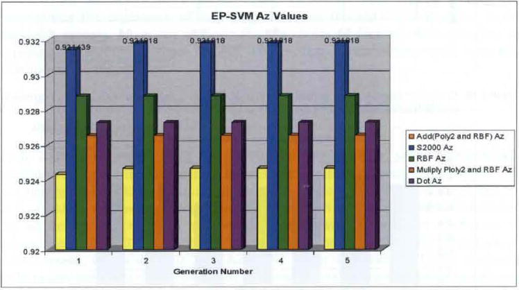
AZ results from EP SVM software package using five fold cross validation (see online version for colours)

Figure 8.

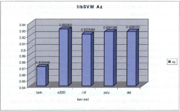
AZ results from Iteratively trained SVM software package using five fold cross validation (see online version for colours)

Biographies

Walker H. Land Jr. is currently a Research Professor in the Department of Bioengineering as well a Principal Investigator and Director of a Computational Intelligence group there. He has over 30 years of industrial research experience and over 25 years of academic research and teaching experience. He is the author/co-author of over 200 peer reviewed research as well as several other publications.

John J. Heine is currently an Associate Professor at the Moffitt Cancer Center and the University of South Florida Tampa, FL. He has over 15 years experience in imaging physics and in the automated statistical analysis of mammograms.

Tom Raway is currently a graduate student in the Department of Bioengineering at Binghamton University and a member of the Computational Intelligence research Group.

Alda Mizaku is currently a graduate student in the Department of Bioengineering at Binghamton University and a member of the Computational Intelligence research Group.

Nataliya Kovalchuk is research associate with the Moffitt Cancer Center and University of South Florida Tampa, FL, 33620 USA.

Jack Y. Yang is with Harvard Medical School, Harvard University. He received his PhD from Purdue University, and his post doctoral training from Harvard University. He was a faculty member at Indiana University. He has published more than 90 peer-reviewed papers and book chapters. He has served as Editor of more than a dozen journals and proceedings. He was a recipient of best papers, outstanding research achievements and educational service awards. He was the invited General Chair of IEEE Bioinformatics and Bioengineering at Harvard Medical School in 2007. He is a computational as well as experimental scientist with more than 15 years of experience in teaching, research and engineering practice. He specialises in artificial intelligence and cancer biology.

Mary Qu Yang is with National Human Genome Research Institute, National Institute of Health. she received her PhD from Purdue University and her post doctor training from National Institutes of Health. She was a recipient of the Outstanding Interdisciplinary Bilsland Dissertation fellow for biological physics and computer engineering dual degrees, the NIH fellow for National Human Genome Research and the NIH – Oak Ridge, DOE fellowship. She received Best Paper, Smart Engineering Systems Design and Theoretical Developments in Computational Intelligence Awards at Artificial Neural Networks in Engineering, as well as Best Software and Best Inter/Multidisciplinary Awards at IEEE Bioinformatics and Bioengineering. She has published more than 80 peer-reviewed papers and has served as an Editor of a number of journals. She specialises in software engineering and genomics.

References

- Agency for Healthcare Research and Quality (AHRQ) Report Effectiveness of Noninvasive Diagnostic Tests for Breast Abnormalities. 2006 Published 02/09/2006, http://effectivehealthcare.ahrq.gov/reports/topic.cfm?topic=2&sid=32&rType=3. [PubMed]
- Awais MM, Shamail S, Ahmed N. Dimensionality reduced Krylov subspace model reduction for large scale systems. Applied Mathmetics and Computation. 2007 Aug;1(1):21–30. [Google Scholar]
- Burges CJC. Data Mining and Knowledge Discovery. Vol. 2. Kluwer; Boston: 1998. A tutorial on support vector machines for pattern recognition; pp. 121–167. [Google Scholar]
- Cristianini N, Shawe-Taylor J. An Introduction to Support Vector Machines and other Kernel-Based Learning Methods. Cambridge University, Cambridge University Press; The Edinburgh Building, CB2 2RU, UK: 2000. [Google Scholar]
- Delogu P, Evelina FM, Kasae P, Retico A. Characterization of mammographic masses using a gradient-based segmentation algorithm and a neural classifier. Comput Biol Med. 2007;37:1479–1491. doi: 10.1016/j.compbiomed.2007.01.009. [DOI] [PubMed] [Google Scholar]
- Elter M, Schulz-Wendtland R, Wittenberg T. The prediction of breast cancer biopsy outcomes using two CAD approaches that both emphasize an intelligible decision process. Med Phys. 2007;34:4164–4172. doi: 10.1118/1.2786864. [DOI] [PubMed] [Google Scholar]
- Floyd CE, Lo JY, Yun AJ, Sullivan DC, Kornguth PJ. Prediction of breast cancer malignancy using an artificial neural network. Cancer. 1994;74:2944–2998. doi: 10.1002/1097-0142(19941201)74:11<2944::aid-cncr2820741109>3.0.co;2-f. [DOI] [PubMed] [Google Scholar]
- Floyd CE, Lo JY, Tourassi GD. Case-based reasoning computer algorithm that uses mammographic findings for breast biopsy decisions. AJR Am J Roentgenol. 2000;175:1347–1352. doi: 10.2214/ajr.175.5.1751347. [DOI] [PubMed] [Google Scholar]
- Fogel DB, Wasson EC, Boughton EM. Evolving neural networks for detecting breast cancer. Cancer Letters. 1995;96:49–53. doi: 10.1016/0304-3835(95)03916-k. [DOI] [PubMed] [Google Scholar]
- Fogel DB, Wasson EC, Boughton EM, Porto VW. A step toward computer-assisted mammography using evolutionary programming and neural networks. Cancer Letters. 1997;119:93–97. doi: 10.1016/s0304-3835(97)00259-0. [DOI] [PubMed] [Google Scholar]
- Fogel DB, Wasson EC, Boughton EM, Porto VW. Evolving artificial neural networks for screening features from mammograms. Artificial Intelligence in Medicine. 1998a;14:317–326. doi: 10.1016/s0933-3657(98)00040-2. [DOI] [PubMed] [Google Scholar]
- Fogel DB, Wasson EC, Boughton EM, Porto VW, Angeline PJ. Linear and neural models for classifying breast masses. IEEE Trans Medical Imaging. 1998b;17:485–488. doi: 10.1109/42.712139. [DOI] [PubMed] [Google Scholar]
- Fogel DB. Evolutionary Compulation: Toward a New Philosophy of Machine Intelligence. IEEE Press; Piscataway, NJ: 1995. [Google Scholar]
- Gunn S. Support Vector Machines for Classification and Regression. ISIS Technical Report, Image Speech and Intelligent Systems Group, University of Southampton; Southampton, England: 1998. May 14, [Google Scholar]
- Haaland DM, Thomas EV. Partial least squares methods for spectral analysis relative to other quantitative calibration methods and the extraction of qualitative information. Analytical Chemistry. 1988;60:1193–1202. [Google Scholar]
- Habas PA, Zurada JM, Elmaghraby AS, Tourassi GD. Reliability analysis framework for computer-assisted medical decision systems. Med Phys. 2007;34:763–772. doi: 10.1118/1.2432409. [DOI] [PubMed] [Google Scholar]
- Ipsen CF, Meyer CD. The idea behind Krylov methods. American Mathematical Monthly. 1998 Dec;105(10):889–899. [Google Scholar]
- Land WH, Masters T, Lo JY, McKee D. Using evolutionary computation to develop neural network breast cancer benign/malignant classification models. 4th World Conference on Systemics, Cybernetics and Informatics. 2000a;10:343–347. [Google Scholar]
- Land WH, Jr, Masters T, Lo JY. IEEE Congress on Evolutionary Computation Proceedings. La Jolla Marriott Hotel, La Jolla, Ca: 2000b. Jul 16–19, 2000. Application of a new evolutionary programming/adaptive boosting hybrid to breast cancer diagnosis; pp. 436–1443. [Google Scholar]
- Land WH, Jr, Heine JJ, Embrechts M, Smith T, Choma R, Wong L. New approach to breast cancer cad using partial least squares and kernel-partial least squares. SPIE Medical Imaging. 2005a;5747:48–57. [Google Scholar]
- Land WH, Jr, Anderson F, Smith T, Falhbusch S, Choma R, Wong L. Applying knowledge engineering and representation methods to improve support vector machine and multivariate probabilistic neural network performance. SPIE M,i. 2005b:895–902. [Google Scholar]
- Land WH, Jr, Tomko GG, Heine JJ. Comparison of logistics regression (LR) and evolutionary programming (EP) derived support vector machines (SVM) and chi squared derived results for breast cancer diagnosis. Intelligent Engineering Systems Through Artificial Neural Networks. 2006;16:267–272. [Google Scholar]
- Lo JY, Baker JA, Kornguth PJ, Iglehart JD, Floyd CE. Predicting breast cancer invasion with artificial neural networks on the basis of mammographic features. Radiology. 1997;203:159–163. doi: 10.1148/radiology.203.1.9122385. [DOI] [PubMed] [Google Scholar]
- Malinowski ER. Theory of error in factor analysis. Analytical Chemistry. 1977;49:606–612. [Google Scholar]
- Martens H, Naes T. Multivariate Calibration. Wiley; New York: 1989. [Google Scholar]
- Mavroforakis ME, Georgiou HV, Dimitropoulos N, Cavouras D, Theodoridis S. Mammographic masses characterization based on localized texture and dataset fractal analysis using linear, neural and support vector machine classifiers. Artif Intell Med. 2006;37:145–162. doi: 10.1016/j.artmed.2006.03.002. [DOI] [PubMed] [Google Scholar]
- Morris EA, Liberman L, editors. Breast MRI Diagnosis and Intervention. Springer; NY: 2005. p. 55. [Google Scholar]
- Nandi RJ, Nandi AK, Rangayyan RM, Scutt D. Classification of breast masses in mammograms using genetic programming and feature selection. Med Biol Eng Comput. 2006;44:683–694. doi: 10.1007/s11517-006-0077-6. [DOI] [PubMed] [Google Scholar]
- National Cancer Institute SEER Cancer. Statistics Review 1975–2003. 2006 Table I-1, Estimated New Cancer Cases and Deaths for 2006, http://seer.cancer.gov/csr/1975_2003/
- Sahiner B, Chan HP, Petrick N, Helvie MA, Hadjiiski LM. Improvement of mammographie mass characterization using spiculation measures and morphological features. Med Phys. 2001;28:1455–1465. doi: 10.1118/1.1381548. [DOI] [PubMed] [Google Scholar]
- Shawe-Taylor J, Cristianini N. Kernel Methods for Pattern Analysis. Cambridge University Press; The Edinburgh Building, CB2 2RU, UK: 2004. Cambridge University Press. [Google Scholar]
- Shi J, Sahiner B, Chan HP, Ge J, Hadjiiski L, Helvie MA, Nees A, Wu YT, Wei J, Zhou C, Zhang Y, Cui J. Characterization of mammographie masses based on level set segmentation with new image features and patient information. Med Phys. 2008;35:280–290. doi: 10.1118/1.2820630. [DOI] [PMC free article] [PubMed] [Google Scholar]
- Strax P. Make Sure That You Do Not Have Breast Cancer. St. Martin’s, NY: 1989. [Google Scholar]
- Timp S, Varela C, Karssemeijer N. Temporal change analysis for characterization of mass lesions in mammography. IEEE Trans Med Imaging. 2007;26:945–953. doi: 10.1109/TMI.2007.897392. [DOI] [PubMed] [Google Scholar]
- Tourassi GD, Harrawood B, Singh S, Lo JY. information-theoretic CAD system in mammography: entropy-based indexing for computational efficiency and robust performance. Med Phys. 2007;34:3193–3204. doi: 10.1118/1.2751075. [DOI] [PubMed] [Google Scholar]
- Verela C, Timp S, Karssemeijer N. Use of border information in the classification of mammographie masses. Phys Med Biol. 2006;51:425–441. doi: 10.1088/0031-9155/51/2/016. [DOI] [PubMed] [Google Scholar]
- Wold H. Path models with latent variables: the NTPALS approach. In: Balock HM, editor. Quantitative Sociology: International Perspectives on Mathematical and Statistical Model Building. Academic Press; NY: 1975. pp. 307–357. [Google Scholar]
- Wold H. Estimation of principal components and related models by iterative least squares. In: Krishnaiah PR, editor. Multivariate Analysis. Academic Press; NY: 1966. pp. 391–420. [Google Scholar]
- Wold S, Sjölström M, Erikson L. PLS-regression: a basic tool of chemometrics. Chemometrics and Intelligent Laboratory Systems. 2001;58:109–130. [Google Scholar]