Using model-based proposals for fast parameter inference on discrete state space, continuous-time Markov processes

Abstract

Bayesian statistics provides a framework for the integration of dynamic models with incomplete data to enable inference of model parameters and unobserved aspects of the system under study. An important class of dynamic models is discrete state space, continuous-time Markov processes (DCTMPs). Simulated via the Doob–Gillespie algorithm, these have been used to model systems ranging from chemistry to ecology to epidemiology. A new type of proposal, termed ‘model-based proposal’ (MBP), is developed for the efficient implementation of Bayesian inference in DCTMPs using Markov chain Monte Carlo (MCMC). This new method, which in principle can be applied to any DCTMP, is compared (using simple epidemiological SIS and SIR models as easy to follow exemplars) to a standard MCMC approach and a recently proposed particle MCMC (PMCMC) technique. When measurements are made on a single-state variable (e.g. the number of infected individuals in a population during an epidemic), model-based proposal MCMC (MBP-MCMC) is marginally faster than PMCMC (by a factor of 2–8 for the tests performed), and significantly faster than the standard MCMC scheme (by a factor of 400 at least). However, when model complexity increases and measurements are made on more than one state variable (e.g. simultaneously on the number of infected individuals in spatially separated subpopulations), MBP-MCMC is significantly faster than PMCMC (more than 100-fold for just four subpopulations) and this difference becomes increasingly large.

1. Introduction

The development, testing and consequent refinement of dynamic mathematical models plays an increasingly important role in the study of many systems. Bayesian statistics provides a general framework for inference of both model parameters and unobserved/unobservable aspects of system dynamics, and gives a rigorous basis for prediction, decision-making and model comparison [1]. As a reliable statistical technique, Bayesian inference, in the context of the type of models studied here, is a well-established methodology for extracting information from biological data (e.g. see [2–4] for epidemiological examples). However, despite the success of applying Bayesian methods to many systems, use has often been limited by computing power. In this paper, we develop novel computationally efficient tools that implement Bayesian inference for discrete state space, continuous-time Markov processes (DCTMPs). As described below, DCTMPs have proved extremely useful in modelling a huge range of biological phenomena. Moreover, the innovative computational approach introduced in this paper leverages the specific structure of the model under study, and therefore has the potential to make an impact across the same broad range of applications.

DCTMPs are readily simulated using the Doob–Gillespie algorithm [5] and have been used to model stochastic dynamics in a wide range of systems, including: a long history of application to human, animal and plant epidemics (see [6] for an overview); the study of population dynamics in ecology [7]; variation in the concentration of various compounds resulting from chemical reactions [5]; financial crises [8]; biochemical networks [9]; gene expression [10] and the behaviour of quantum systems [11]. Gibson & Renshaw [11,12] demonstrated implementation of Bayesian inference for DCTMPs by applying Markov chain Monte Carlo (MCMC) methods, and this now standard approach has subsequently been employed to conduct inference in epidemics [13], ecology [14] and systems biology [15].

The computational costs of implementing Bayesian inference using MCMC have led to the development of alternative approaches including approximate Bayesian computation (ABC) [16] and methods based on particle filtering such as particle MCMC (PMCMC) [17]. In addition, several authors have attempted to enhance Bayesian inference for continuous state space dynamical systems by modifying MCMC to use local gradients in the posterior distribution [18,19]. By contrast, this paper proposes a more effective MCMC proposal to implement Bayesian inference in discrete state space dynamical systems and specifically for DCTMPs.

We begin with a brief review of DCTMPs (§2) and Bayesian inference on these systems (§3). Section 4 details the computational approaches used to achieve this inference: a standard MCMC algorithm, PMCMC and MCMC using a new proposal type that is computationally more efficient than the standard approach. This new proposal, termed a ‘model-based proposal’ (MBP), represents the important novel aspect of this paper. These MBPs are generically applicable to DCTMPs, but for clarity of exposition are introduced and demonstrated in the context of two simple models that are widely used in epidemiology. A numerical comparison of all three techniques is given in §5, the paper is summarized in §6 and, finally, we discuss future research possibilities in §7.

2. Discrete state space, continuous-time Markov processes

Consider the following generic DCTMP in which, at time point t, the system state can be represented by a vector n(t) that contains N state variables. Each variable represents the population size in the N compartments within the model. Because populations take integer values, the space of possible configurations that the system can potentially take is discrete. Transitions of individuals between compartments are also discrete and are captured by E possible event types. Each event type e has the effect of altering the state variables as follows:

2.1

where c denotes one or more compartments changed by the event and Q is a fixed matrix. The average rate at which each event type occurs is defined by the elements of vector r(t). An important simplifying assumption in DCTMPs is the Markovian property, which assumes that these rates are solely dependent on the current state vector n(t), rather than on any previous state of the system.¹ The functional dependence between r(t) and n(t) is characterized by parameters collectively referred to as θ.

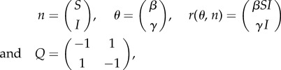
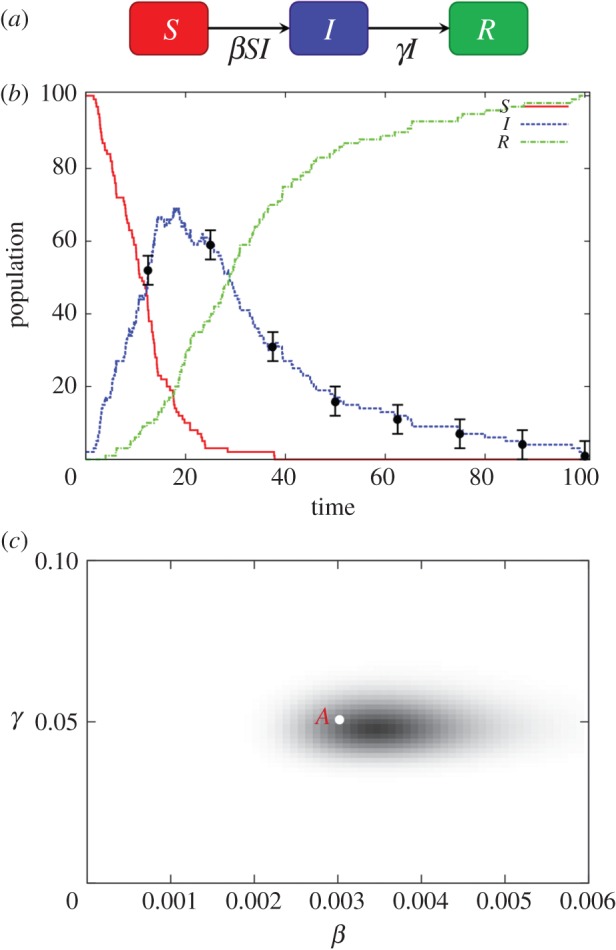
To give an example, a commonly used compartmental model in epidemiology is the SIS model, illustrated in figure 1a. This divides individuals into those that are not infected and are susceptible to infection (the ‘S’ compartment) and those that are infected and infectious (the ‘I’ compartment). In this model, two possible events can occur: an infection (S is reduced by one and I increased by one) or a recovery (I is reduced and S is increased). Such a model is relevant to infections such as the common cold or influenza, which do not confer long-lasting immunity. For the SIS model in figure 1a, the following definitions can be made:

2.2

where event 1 is infection and event 2 is recovery.

Figure 1.

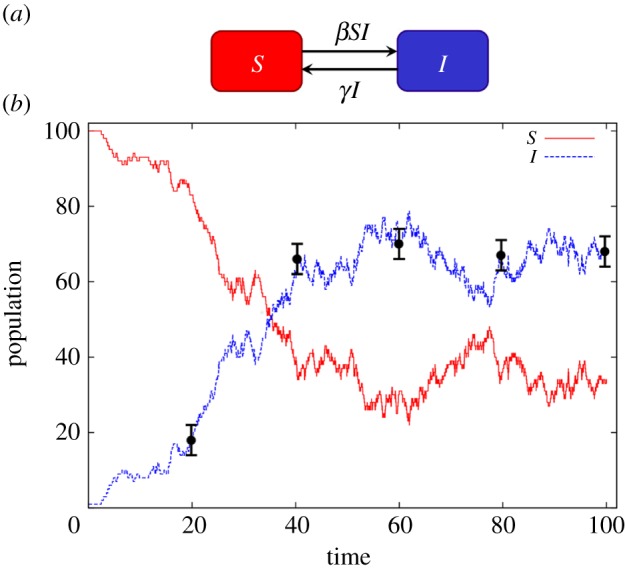
(a) The SIS compartmental model. S represents the population of individuals susceptible to an infection and I the infected population. The arrows represent movement of individuals between compartments. The average rate of infections and recoveries is given by βSI and γI, respectively. (b) A single realization of the dynamics of the system as modelled using the Doob–Gillespie algorithm with parameters β = 0.003 and γ = 0.1. The black circles denote hypothetical measurements made on the infected population and the error bars the associated uncertainty in these observations. (Online version in colour.)

This model can be simulated using the Doob–Gillespie algorithm (subsequently abbreviated as DGA), a standard stochastic simulation technique for generating event sequences from DCTMPs (see the electronic supplementary material, appendix A, for details). Results are shown in figure 1b for the case in which a single infected individual enters a population of 100 susceptible individuals (corresponding to an initial state vector n^init = n(0) = (100, 1)). The parameters used were θ = (β, γ) = (0.003, 0.1), with simulation time T = 100. An initial rapid increase in the infected population (dotted curve) settles towards an endemic scenario, in which the rate of infection and recovery events approximately balance.

The black circles in figure 1b denote potential estimates of the infected population size I, made at discrete time intervals. For this study, these data points are used as hypothetically observed data ‘y’, which are collected over the time period [0, T]. The error bars associated with the circles in figure 1b represent the uncertainty associated with these measurements.² In general, measurements on state variables are not necessarily regularly spaced, as in figure 1b, and can be made on different compartments at different times. For m ranging from 1 to M, we take c_m to represent the compartment measured with τ_m the time of measurement, v_m the observed value of the state variable (i.e. the population size in compartment c_m at time τ_m) and σ_m the uncertainty associated with the measurement. For example, the first measurement in figure 1b is defined by c₁ = I, τ₁ = 20, v₁ = 18 and σ₁ = 2. The hypothetical data in figure 1b is later used to provide a benchmark against which to assess the relative performance of the three computational approaches.

It should be stressed that these algorithms can be applied to arbitrary DCTMP. The simple SIS outlined above, and SIR and meta-population SIR models later used, have been selected for the purposes of clearly identifying the relative strengths and weaknesses of each approach. The implications of this analysis, however, are vitally important in developing practical Bayesian inference techniques for the wide range of applications identified in Introduction.

3. Bayesian framework

The data y from the previous section is insufficient to determine the precise sequence of events ξ and parameter values θ used to generate it. Bayesian analysis [1] assesses the probability, conditional on the model and the data, that the parameters θ and the so-called latent (unobserved) variables ξ take particular values. Using Bayes' theorem, this probability, termed the posterior, can be written as

3.1

Here, π(ξ|θ) represents the probability that a DGA simulation (as outlined in electronic supplementary material, appendix A) of the model using parameters θ generates event sequence ξ. It can be expressed as (see below for a brief derivation) [12,20]:

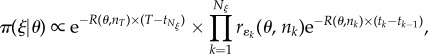3.2

where the product runs over all N_ξ events in ξ. The quantities t_k and ɛ_k represent, respectively, the time and type (i.e. infection or recovery for the SIS model) of each event. The rates r(θ, n_k), such as those given in equation (2.2), are evaluated using parameters θ and the state vector n_k immediately prior to time t_k. R(θ, n_k) = Σ_er_e(θ, n_k) is the total event rate. We define t₀ = 0 as the time at which the initial conditions are set.

Equation (3.2) can be derived by considering the two ways in which stochasticity enters the DGA (see electronic supplementary material, appendix A): (1) event times are drawn from the exponential distribution P(t_k) = R(θ, n_k)exp(−R(θ, n_k) × (t_k − t_k−1)) and (2) event types are selected with probability P(ɛ_k) = r_ɛk(θ, n_k)/R(θ, n_k). Multiplying these terms for all events in ξ leads to equation (3.2). The first term on the right-hand side of equation (3.2), where n_T represents the final state vector of the system, accounts for the time between the last event and the final observation time T.

The probability of measuring data y given that the actual system has event sequence ξ is given by π(y|ξ), referred to as the observation model. If we assume a simple normal distribution³ in the error of a single measurement y_sing, the probability of observing a population value v given it actually has a value n is

3.3

where n and σ² are the mean and variance of a normal distribution (see electronic supplementary material, appendix B, for a definition of this function). If we assume that the M measurement errors in y are uncorrelated,⁴ the observation model for the complete data y can be written as the product

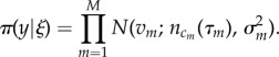3.4

This term contributes to the posterior probability equation (3.1) by giving greater weight to event sequences ξ that pass near to the measurements.

In the Bayesian framework, previous knowledge about model parameters is encapsulated in the prior distribution π(θ) in equation (3.1).⁵ A flat uninformative prior is assumed for the numerical results in this study.

Figure 2 shows a two-dimensional representation of the posterior distribution marginalized in parameter space π(θ|y), as discretized on an 80 × 80 grid, for the SIS model with θ = (β, γ) assuming data y from figure 1b. Darker shaded regions indicate more probable parameter combinations that are consistent with the observed data, model and prior. Point A represents the parameter values used to generate the true event sequence. This point lies within the shaded area, indicating that there is sufficient information within the measurements to approximately infer the true parameter values underlying the system's dynamics.⁶

Figure 2.

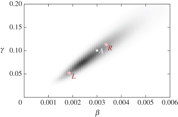
The posterior distribution in parameter space. Point A represents the parameters used to generate the data in figure 1b. Points L and R represent regions at either end of the posterior (see electronic supplementary material, appendix E, for details). (Online version in colour.)

4. Material and methods

We now describe three different algorithms to generate the plot shown in figure 2. Standard MCMC and the PMCMC methods are briefly described below (details in the electronic supplementary material), and then the new MBP technique, which represents the novel contribution of this paper, is presented in some detail.

4.1. Standard Markov chain Monte Carlo

The standard method consists of generating an MCMC chain of event sequences ξⁱ and parameters values θⁱ (where i denotes the position on the chain) using proposals randomly selected from four possibilities: (1) change a parameter value, (2) insert an event, (3) remove an event or (4) change the time of an event. Details of this procedure are given in electronic supplementary material, appendix C. These changes permit the algorithm to explore complete parameter and event space, and the resulting chain is guaranteed to asymptotically be distributed in accordance with the posterior probability, i.e. in the limit as the number of iterations goes to infinity.

The dotted-dashed line in figure 3a illustrates an example of an output from the standard MCMC algorithm, above. This shows the sequence of samples generated for β based on the data from the SIS model example in figure 1b. Observe that the curve moves up and down very slowly (note the large number of iterations on the x-axis). Within MCMC, the process whereby parameters explore the posterior is known as ‘mixing’. The problem of slowly varying parameters, or poor mixing, results from consecutive samples in the Markov chain being highly correlated (see [15] for another example). Mixing may be quantified through the autocorrelation function R (described in electronic supplementary material, appendix G). This is plotted as a function of CPU time in figure 3b (time is used instead of sample number to allow a direct comparison with the other methods, later). The dotted-dashed curve shows that after 1 s of computation (corresponding to around 5200 MCMC iterations), R = 0.96, indicating that the chain is still highly correlated over this timescale. (An intuitive explanation for this high degree of autocorrelation is presented in electronic supplementary material, appendix E.)

Figure 3.

(a) Trace plots for the variation in β as a function of iteration number generated using the three inference methods with measurements from figure 1b. PMCMC is found to mix best, MBP-MCMC not quite as well and the standard MCMC mixes extremely slowly (note the much longer timescale). (b) The autocorrelation in β, approximated using electronic supplementary material, equation (D1) for C = 10⁷ iterations, as a function of CPU time. (Online version in colour.)

4.2. Particle Markov chain Monte Carlo

PMCMC is a recently proposed technique that exploits knowledge of the model and is naturally parallelizable. Its operation reduces the problematic correlations in event sequences found above [17], and application of PMCMC to compartmental models has recently been proposed [21,22]. The actual operation of PMCMC comes in two main varieties described below.

4.2.1. Particle marginal Metropolis–Hastings

This approach treats parameters and event sequences somewhat differently. In terms of events, a sequential Monte Carlo (SMC) method [23] takes a given set of parameter values θ and simulates a series of possible event sequences, or ‘particles’, from the model. At measurements, a so-called ‘particle filter’ is applied to prune those generated sequences that are not in good agreement with the data. An overall measure of how well the simulated event sequences agree with the data y provides an unbiased estimate of the posterior distribution marginalized in parameter space In PMCMC, exploration in parameter space is achieved through an MCMC scheme that uses the approximation rather than the full posterior π(θ, ξ|y). A consequence of this approach is that event sequences become largely uncorrelated between subsequent iterations of the MCMC chain. This benefit in terms of mixing, however, comes at the significant computational cost of simulating the system multiple times. Further details of particle marginal Metropolis–Hastings (PMMH) are presented in electronic supplementary material, appendix F, and suitable optimization (e.g. selecting particle number) is described in electronic supplementary material, appendix H.

4.2.2. Particle Gibbs

Iteratively, SMC is used to draw samples from π(ξ|y,θ) (by means of a Metropolis–Hastings step) and Gibbs (for cases in which it is possible) is used to directly sample from π(θ|ξ). For typical DCTMPs, there is a high degree of correlation between model parameters and state space. This leads to the Gibbs step only proposing relatively small jumps in parameter space (demonstrated by the fact that the distribution π(θ|ξ) in electronic supplementary material, figure 3, is much smaller than the full posterior shown in figure 2), resulting in highly correlated PMCMC samples. Consequently, the particle Gibbs version of PMCMC was found to be much less efficient than the PMMH procedure above, and the results presented here are obtained solely from the latter.

The dashed curve in figure 3a shows the variations in β, again based on the data from figure 1b. Observe that this curve moves up and down much more quickly than the standard MCMC method (note the different scales on the x axes). Although it takes significantly longer to run per iteration, it is a superior algorithm. This finding is emphasized by the autocorrelation function in figure 3b, which shows that the MCMC chain becomes largely uncorrelated after approximately half a second of computation time.

4.3. Model-based proposal Markov chain Monte Carlo

Above we demonstrated that the standard MCMC procedure is an inefficient means of obtaining posterior estimates for DCTMPs due to the strong autocorrelation of samples. Because event sequences and parameter values are highly correlated, any efficient scheme must simultaneously change parameters and events during the proposal step. Here, we present a generic method that achieves this by first proposing a large jump in parameter space θ^f and then constructs a suitable event sequence ξ^f based on θ^f, θⁱ and ξⁱ. The algorithm is as follows.

4.3.1. Initialization

Initial parameter values θ¹ and event sequence ξ¹ are set. These may be generated by first randomly assigning plausible values for θ¹ (perhaps guided by a prior distribution) and then simulating ξ¹ using the DGA. In this study, we simulated an event sequence to generate data y in the first place (figure 1b), so it was convenient to use this for ξ¹. (It should be stressed, however, that arbitrary choice of ξ¹ would be equally valid, and this decision has no impact on the results presented in this paper because the system is sufficiently burned in before samples are taken.)

4.3.2. Step 1

Generate θ^f based on θⁱ. Many possibilities exist, but for this study we use a multivariate normal jumping distribution centred at θⁱ scaled by a jumping size j_F:

4.1

The covariance matrix Σ of the posterior distribution in parameter space is numerically approximated during the adaptation phase (see electronic supplementary material, appendix H, for details) along with an optimal choice for j_F. The advantage of using a multivariate distribution (rather than a simple normal of for each parameter separately) is because it accounts for potential correlations between parameters which would otherwise restrict jumping size.

4.3.3. Step 2

Generate event sequence ξ^f using ξⁱ, θ^f and θⁱ. The essential concept is to construct a new sequence of events that is representative of that generated from the model using θ^f, based on the assumption that ξⁱ is representative of that generated using θⁱ. This represents the key novel aspect of this algorithm. The approach is illustrated in figure 4. At time t = 0, we initialize the state vectors for both the existing sequence and the proposed sequence n^f(0) = nⁱ(0) = n^init. The difference in rates between the two sequences for each event type e is calculated as:

4.2

Figure 4.

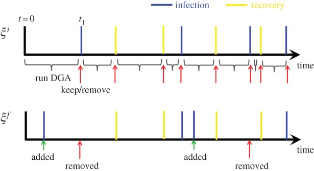
Illustrates the generation of the proposal event sequence ξ^f from an initial sequence ξⁱ in MBPs. Events are added and removed in accordance with step 2 of §4. (Online version in colour.)

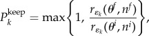
Note, the max function ensures that this quantity is always non-negative and represents the excess rate for each event type at θ^f compared with θⁱ. The DGA is run based on Δr_e(t) (as opposed to the usual r_e(t)) up to the first event time (see t₁ in the sequence ξⁱ in figure 4). This potentially adds new events to the timeline, e.g. a new infection event is added to ξ^f in the diagram. Next, we assess whether or not to copy the event present in ξⁱ (e.g. at t₁) into ξ^f (this accounts for cases when the rates at θ^f are lower than that at θⁱ). This copying is done with probability

4.3

where k is the event number on sequence ξⁱ, which at t₁ is k = 1 (figure 4). The process of running the DGA based on Δr_e to insert new events (represented by the curly brackets on the timeline in figure 4) and probabilistically copying events using equation (4.3) (represented by the arrows in the diagram) is repeated until the maximum observation time T is reached.

It should be noted that the procedure above applies to arbitrary DCTMP, and not simply the models investigated in this paper.

4.3.4. Step 3

Accept or reject the proposal. Set ξⁱ⁺¹ = ξ^f and θⁱ⁺¹ = θ^f with Metropolis–Hastings probability

4.4

else ξⁱ⁺¹ = ξⁱ and θⁱ⁺¹ = θⁱ. Two important points can be made about this expression. Firstly, it is proportional to the ratio of observation model probabilities equation (3.4) for the two event sequences π(y|ξ^f) and π(y|ξⁱ). Therefore, sequences in better agreement with the observations will be preferentially selected. Secondly, equation (4.4) does not contain the event sequence probability from equation (3.2), unlike the corresponding Metropolis expression used in the standard MCMC method. This is because the model, itself, is used to generate the proposal in step 2 above,⁷ and consequently terms in the event sequence probability and proposal distribution cancel each other out (as shown in electronic supplementary material, appendix J).

4.3.5. Step 4

Increment i and jump to step 1 or stop if sufficient accuracy has been achieved.

An example implementation of the MBP procedure written in C++ has been placed in the electronic supplementary material (download the file MBPexample.cc).

The solid curve in figure 3a shows how β varies as a function of iteration number for model-based proposal MCMC (MBP-MCMC). We observe that it does not mix quite as well as PMCMC, but because it is computationally faster per iteration,⁸ the autocorrelation function in figure 3b shows the MBP method to be significantly less autocorrelated than PMCMC at short computational timescales and it does not exhibit the same long tail.

A key justification for the procedure outlined in steps 1 and 2 above is that it ensures the acceptance probability in equation (4.4) does not contain the model, but rather only the data y, the current and proposed event sequences, and the prior. The model is incorporated into the proposal, hence the terminology ‘model-based’ proposal. This has important implications. Supposing no measurements are made on the system (i.e. π(y|ξ) = 1), repeated application of MBPs result in the Markov chain mapping out the prior distribution, as would be expected. Importantly, however, j_F in equation (4.1) can be chosen to propose arbitrarily large jumps in parameter space. These large jumps mean that consecutive samples on the MCMC chain are highly uncorrelated, and hence mixing is good. This is in stark contrast with proposals that use the normal Metropolis–Hastings expression, which relies of calculating event sequence probabilities. Here, even in the absence of measurements, the proposal jumping size is typically highly restricted by the model (because large jumps in either parameter space or state space have a very low probability of acceptance), leading to poor mixing. In reality, of course, any meaningful Bayesian analysis requires measurements. But because the number of observations is typically much smaller than the number of events in the system, a Metropolis–Hastings acceptance rate based on the ratio of observation model probabilities is much less restrictive that one based on the ratio of event sequence probabilities.

5. Results

Simulations were performed to assess the speed and accuracy of the three algorithms presented in §4 (standard MCMC method, PMCMC and MBP-MCMC). An efficient scheme for plotting the posterior distribution (based on Rao–Blackwellization) is outlined in electronic supplementary material, appendix G. Assessing the accuracy of this distribution after a certain number of iterations of a given algorithm presents difficulties because there is no analytical expression available with which to compare the results. Consider, however, running W different versions of the algorithm. They are each started with a different random seed⁹ and so the approximations to the posterior they generate are different. In the asymptotic limit, these approximations all converge to the actual posterior. The efficiency of each algorithm is evaluated by how quickly this convergence occurs (electronic supplementary material, appendix L, describes how this measure is defined).

Figure 5 shows how average posterior accuracy improves as a function of CPU time¹⁰ (based on a 2 GHz processor) for the three methods when using the data from figure 1b (note the log–log axes). Here, W = 50 chains are used and the MBP-MCMC, PMCMC and standard MCMC methods are iterated for 6 × 10⁵, 10⁵ and 6 × 10⁶ steps, respectively. An adaptation phase of 10⁵ iterations is used to ensure each method uses optimized constants and is sufficiently burned in.

Figure 5.

Shows how the accuracy of the posterior estimate improves with CPU time for the three different methods. The black arrows indicate the average autocorrelation times, and The thin black line, with slope −1/2, shows the expected long-term scaling behaviour. (Online version in colour.)

Consider the solid curve representing the MBP-MCMC results. Initially, the accuracy remains fairly flat, which can be interpreted as the time over which the chain mixes (the average autocorrelation times, as defined in electronic supplementary material, appendix G, for the three methods are denoted by the black arrows). In the long time limit, the curve approaches its theoretically expected slope¹¹ represented by the thin black line. An accuracy of 10% is taken to correspond to an acceptable approximation of the posterior. We see from the black dot in figure 5 that MBP-MCMC takes around 52 s of calculation to achieve this. Compare now the dashed line for the PMCMC results in figure 5. This is shifted to right of the solid curve, hence it is slower. To achieve the same 10% accuracy requires around 295 s of computation, almost six-times longer. This increase is mainly due to the fact that it was necessary for p = 20 particles to be used, hence the DGA was effectively simulating the model 20 times per PMCMC step. The dotted-dashed line shows the results from the standard MCMC method. It is vastly slower than the other two methods, and it was not feasible to achieve an accuracy of 10%. However, an estimate of the time it would have taken is obtained by fitting a line of slope −1/2 to the final point on the curve and extrapolating, an approximation that is used in the subsequent analysis.

Next, we discuss how the three methods compare in various limits. Figure 6a shows how the computation time needed to achieve an accuracy of 10% varies as a function of measurement uncertainty (i.e. the error bar sizes in figure 1b, which are set to a constant value σ_m). The solid curve presents results for MBP-MCMC, showing that reducing σ_m from moderate to small values increases CPU time. This is because it becomes necessary to reduce the proposal jumping size j_F in step 1 of §4 to retain a good chance of acceptance, which leads to longer mixing times. The reason large jumps in parameter space are not permitted is that the method for generating ξ^f does not take into account the data y, so changing many events inevitably leads to a large discrepancy between the observation and what ξ^f suggests really happened, i.e. π(y|ξ^f) in equation (4.4) becomes small. When σ_m increases from moderate to large values in figure 6a, the simulation time also increases, but for a different reason. Due to greater uncertainty in the measurements, the size of the posterior distribution enlarges. Correspondingly, the jumping size gets larger, but not at the same rate, again leading to longer mixing times.

Figure 6.

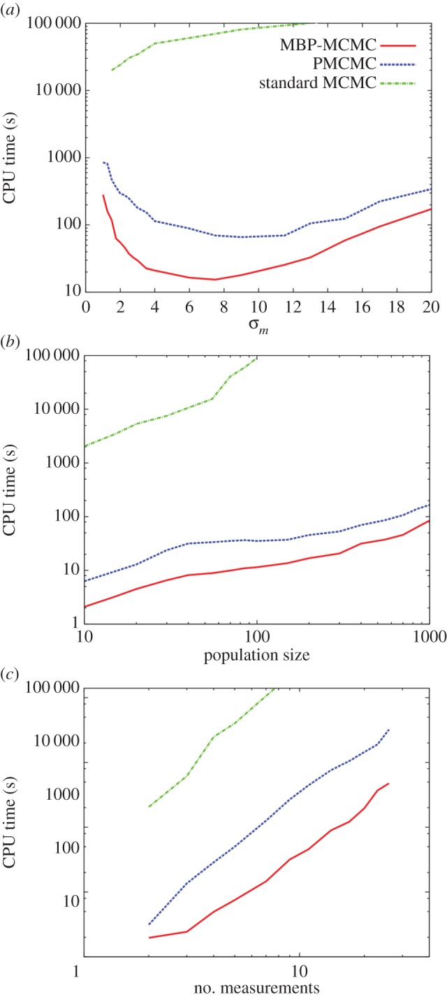
Shows how the CPU time to achieve an accuracy of 10% varies under three different scenarios: (a) the uncertainty in the measurements σ_m is changed, (b) the population size is changed and (c) the number of measurements is changed, assuming a constant time between measurements (hence, the observation period T is also changed). (Online version in colour.)

The situation for the PMCMC simulations, as shown by the dashed curve in figure 6a, is similar although the underlying mechanisms are different. In the case of small σ_m, most, if not all, the particles end up sufficiently far from the measurements that they have a very low observation probability and hence they do not represent samples from the posterior. This results in a larger number of particles being needed to achieve a sufficient accuracy for hence a longer simulation time. The dotted-dashed curve shows that the standard MCMC method is much slower. However, in this case, it becomes faster as σ_m → 0 because the reduction in the size of the posterior more than compensates for the reduction in acceptance rate resulting from the stricter limitations imposed by the observations.

Figure 6b shows the case when the initial susceptible population size S^init is varied. The initial infected population is taken to be I^init = S^init/10, rounding to the nearest integer. S^init was set to have values varying between 10 and 1000. The size of the measurement error was also adjusted to maintain a constant relative error using

5.1

The results were averaged over 10 datasets generated using DGA simulations, with measurements taken at five time points separated at 20 time unit intervals. The speed of PMCMC and MBP-MCMC were found to vary in a similar way. The increase in CPU time is less than linear with S^init because the size of the posterior distribution shrinks as a result of the scaling used in equation (5.1).

Next, we investigate how the computation time depends on the number of measurements made on the system, assuming a constant time difference between them. Figure 1b shows the scenario in which five measurements are made. We now consider what happens if further measurements to this system are added at times τ₆ = 120, τ₇ = 140, etc… (i.e. at 20 time unit intervals). Alternatively, measurements can be removed from this diagram, starting from τ₅ = 100. Results from this process are summarized in figure 6c. We find that MBP-MCMC scales similarly to PMCMC as the number of measurements is changed.

The new MBPs can equally be applied to other compartmental models. For example, figure 7a shows perhaps the most well-known example, the SIR model [6]. In this case, recovered individuals no longer become susceptible, but enter a ‘recovered’ compartment. This model is applicable to diseases which confer lifelong immunity on the host, such as measles or mumps. An example of such system dynamics is given in figure 7b in which a single infected individual enters a susceptible population. An initial explosion in infections (i.e. an epidemic) leads to exhaustion of the susceptible population, after which the remaining infected individuals slowly recover. As in figure 1b, we take the circles in figure 7b as the basis of hypothetical data. Figure 7c shows the posterior distribution generated using MBP-MCMC. Investigation of the scaling shows broadly the same behaviour as in figure 6, although the inference times are much shorter due to fewer events occurring than in the previous SIS example.¹² MBP-MCMC is marginally faster than PMCMC and they are both much quicker than the standard MCMC technique (results not shown).¹³

Figure 7.

(a) The SIR compartmental model with susceptible (S), infected (I) and recovered (R) subpopulations. The arrows represent the possible movement of individuals between compartments. The average rates of infections and recoveries are given by βSI and γI, respectively. (b) A typical DGA simulation from the model which used parameters β = 0.003 and γ = 0.05. The black circles represent hypothetical data. (c) The posterior distribution generated using MBP-MCMC (10⁶ iterations were used), where point A represents the parameters used to generate the data. (Online version in colour.)

Lastly, we look at the scenario in which measurements are made on more than one state variable simultaneously. Figure 8a shows an example of this, which represents a spatial one-dimensional meta-population model. Here, several different spatial regions are considered (two shown in the diagram) whose dynamics are locally described by SIR models. Movement of individuals, characterized by a migration parameter μ, result in a coupling between neighbouring regions. The diagram in figure 8a can be extended to include any number of linked regions in a line. This simple one-dimensional model may, for example, represent different populations along a coastline in which the habitat restricts the population to lie close to the sea. Figure 8b shows an example of the dynamics exhibited by this model, using three regions. An infected animal is initially assumed in the first region, and this leads to an epidemic (see the dark peak on the left). For clarity, the curves showing variation in the susceptible and recovered populations have been omitted. Due to migration of infected individuals to the second region, this initiates a second epidemic occurring at a slightly later time, as shown by the middle peak, and finally in the third region (light peak on the right).

Figure 8.

(a) A one-dimensional meta-population SIR model. The system consists of a number of spatially separated regions whose dynamics are locally described by SIR models. These regions are linked by nearest neighbour migration of individuals at per capita rate μ. (b) A typical realization of the dynamics of the system for the case of three meta-populations as modelled using the DGA with parameters β = 0.003, γ = 0.05 and μ = 0.01. For clarity, only the curves for the infected populations I₁, I₂ and I₃ are shown. (c) How the CPU time required to achieve an accuracy of 10% for the joint posterior distribution in the (β,γ) plane varies as a function of the number of meta-populations. (Online version in colour.)

The circles in figure 8b represent hypothetical measurements made on the system. As in figure 7b, we assume that eight periodic measurements are made, but here they are made simultaneously across all regions. Based on these observations, the posterior distribution in the (β,γ) plane can be established using the approach outlined above (equally it would be possible to investigate inference on parameter μ). Figure 8c shows how the computational time taken to calculate this distribution within 10% depends on the number of regions being observed. We find for PMCMC that this dependency is exponential, and calculation becomes computationally demanding beyond four regions. Using MBP-MCMC, however, the computational time grows much more slowly. This indicates that MBPs can be useful applied to scenarios in which it is not realistically possible for PMCMC to give acceptable results.

6. Summary and conclusion

This paper addresses the computational challenge of generating samples from posterior distributions which arise when conducting Bayesian inference on DCTMPs.

MCMC can be used to implement such inferences [9,11] by constructing a Markov chain to explore the joint space of parameters and events. Standard MCMC approaches typically make independent proposals to the parameters and event sequence, and changes to the event sequence use simple proposals such as adding, deleting or moving individual events. Proposals are retained or rejected according to a Metropolis–Hastings probability. However, if changes in parameter and event space are proposed independently, large changes are typically rejected due to the strong dependence of probable event sequences on parameter values. This means only small changes are likely to be accepted and the algorithm explores the posterior distribution very slowly via a diffusion-like trajectory.

Here, we proposed a generic approach applicable to any DCTMP model to mitigate this problem which generates joint proposals of parameters and event sequences by exploiting the dynamics of the underlying model. Specifically, in MBP-MCMC when a parameter change is proposed, the model dynamics are used to construct a corresponding event sequence proposal. With such MBPs, even large changes have a relatively high acceptance rate and this enables a rapid exploration of the posterior. This novel approach was compared with a standard implementation of MCMC for DCTMPs and a recently proposed PMCMC technique [12].

Often previous attempts to develop complex proposals to help ameliorate mixing problems depend sensitively on exactly how they are implemented for each new model. One of the key advantages of MBPs is that for arbitrarily complex models, only a single tuneable parameter exists (j_F defining the jumping size in parameter space) which can easily be optimized to give a good acceptance rate. Thus, the MBP-MCMC method adapts to the structure of different models.

Homogeneous SIS and SIR models and a meta-population SIR model were used as benchmark computational tests for the three methods. The following conclusions are drawn:

• — standard MCMC is extremely slow for all but the simplest models. It was found to be several orders of magnitude slower than MBP-MCMC and PMCMC;

• — PMCMC and MBP-MCMC had comparable performance when measurements were made on a single compartment (with MBP-MCMC having a slight advantage). They were found to scale in the same way under variation in measurement uncertainty, measurement number and population size; and

• — when measurements were simultaneously made on several state variables (as in, for example, a spatial meta-population model), MBP-MCMC was much faster than PMCMC.

7. Discussion

This paper has presented the case for a new type of generic MCMC proposal (termed ‘MBP’) used to speed up Bayesian inference on DCTMPs. This new proposal has the advantage of having only a single tuneable parameter (making optimization straightforward) and is applicable to arbitrarily complex models. Comparisons were made with standard MCMC and PMCMC approaches, and MBP-MCMC was clearly demonstrated to be significantly computationally faster. Although most of these comparisons were done in simple non-spatial models (the SIS and SIR models), a final application looking at a meta-population model demonstrates that MBPs can, indeed, be scaled up to more complex models. Furthermore, the relative difference in speed between MBP-MCMC and PMCMC was found to increase with larger model complexity, pointing to the fact that MBPs will permit rigorous statistical inference in complex problems that have so far remained computationally infeasible.

Within this paper, MBP-MCMC is compared to the simplest and most widely used version of PMCMC, namely PMMH. This uses a simple SMC scheme that simulates directly from the model and applies a particle filter after each measurement. As pointed out in [17], more advanced SMC techniques and particle filtering procedures have been developed, and these may improve the performance of PMCMC (at the expense of increased algorithm complexity). One strong possibility to improve efficiency is to generate a modified ‘simulation’ that, to some extent at least, takes into account the next set of observations (rather than simulating directly from the model in the SMC step). This may permit PMCMC to overcome its main shortcoming, namely being unable to cope well with multiple simultaneous measurements. However, due to the nonlinear nature of the models, these improved proposals are challenging to be made sufficiently computationally fast to be of practical use.

Another approach that shares the same fundamental aims as MBPs (i.e. to simultaneously propose changes in parameter values and the event sequence) is known as non-centred MCMC [24,25]. Here, the strict separation between model parameters and event sequence times is broken through reparametrization. A simple example, presented in [24], considers the SIR model in which recovery times are known. The difference in the recovery and infection times is assumed to be exponentially distributed. One way to represent the system is to consider some new quantity U drawn from a unit time exponential distribution, and from this reconstruct the infection times as the recovery time minus U/γ. Thus, proposed changes in γ simultaneously alter infection times. In complex problems many different reparametrizations often exist, and it can be challenging to ascertain the best approach. A key advantage of MBPs is that they can be applied to arbitrary DCTMP models without the need to consider this flexibility. Furthermore, unlike non-centred approaches, the jumping probabilities in MBPs (see equation (4.4)) are independent of model complexity and constrained solely by the observation model and prior.

We now briefly discuss ABC in relation to the methods applied in this paper. In particular, we show that there is no reason to believe it can be computationally faster than PMCMC for DCTMPs. One of the key advantages of ABC is that it is a likelihood-free approach. For the models investigated here, however, calculating the likelihood (which is effectively achieved in equation (3.2)) is actually significantly faster than performing a single simulation from the model. The simplest type of ABC algorithm, called the ‘rejection algorithm’, consists of sampling parameter values from the prior, simulating the model using these values and then accepting or rejecting the resulting event sequence depending on some statistic that characterizes how near it falls to the measurements (crudely implementing the observation model in equation (3.4) by, for example, introducing a cut-off observation probability ɛ below which the sample is rejected). Since during this study, we assume no prior knowledge regarding parameter values, this would mean that in order to identify the posterior distribution in figure 2, it would be necessary to randomly select points within this diagram (in a scatter-gun approach), the vast majority of which would have almost zero posterior probability. To overcome this highly inefficient approach, the ABC-MCMC approach has been introduced (e.g. [26]). This is essentially the same as PMCMC but using only a single particle (with the crude implementation of the observation model), and therefore would not be expected to be faster than PMCMC, and in some circumstances (when ɛ becomes smaller) would be much slower.

The concepts underpinning MBPs may be applicable to coarse-grained models of DCTMPs, for example by applying the tau-leaping method [27] or through the use of stochastic differential equations to model the dynamics of the system [21]. Furthermore, extensions of MBPs to generic non-Markovian stochastic discrete event-based models should be relatively straightforward. In addition, the construction of different MBPs (i.e. modifications to step 2 in §4) that satisfy the condition equation (4.4) would permit the application of this new approach to a much wider range of statistical models. These promising developments remain the subject of future work.

Competing Interests

We declare we have no competing interests.

Funding

We wish to thank the Scottish Government for funding through the Strategic Partnership in Animal Science Excellence (SPASE) and the BBSRC through the Institute Strategic Programme Grant.

References

- 1.Box GEP, Tiao GC. 1973. Bayesian inference in statistical analysis. Reading, MA: Addison-Wesley Publishing Co. [Google Scholar]
- 2.Lekone PE, Finkenstadt BF. 2006. Statistical inference in a stochastic epidemic SEIR model with control intervention: Ebola as a case study. Biometrics 62, 1170–1177. ( 10.1111/j.1541-0420.2006.00609.x) [DOI] [PubMed] [Google Scholar]
- 3.Cauchemez S, Carrat F, Viboud C, Valleron AJ, Boelle PY. 2004. A Bayesian MCMC approach to study transmission of influenza: application to household longitudinal data. Stat. Med. 23, 3469–3487. ( 10.1002/sim.1912) [DOI] [PubMed] [Google Scholar]
- 4.Dukic V, Lopes HF, Polson NG. 2012. Tracking epidemics with Google flu trends data and a state-space SEIR model. J. Am. Stat. Assoc. 107, 1410–1426. ( 10.1080/01621459.2012.713876) [DOI] [PMC free article] [PubMed] [Google Scholar]
- 5.Gillespie DT. 1977. Exact stochastic simulation of coupled chemical reactions. J. Phys. Chem. 81, 2340–2361. ( 10.1021/j100540a008) [DOI] [Google Scholar]
- 6.Keeling MJ, Rohani P. 2008. Modeling infectious diseases in humans and animals. Princeton, NJ: Princeton University Press. [Google Scholar]
- 7.Pulliam HR. 1988. Sources, sinks, and population regulation. Am. Nat. 132, 652–661. ( 10.1086/284880) [DOI] [Google Scholar]
- 8.Demiris N, Kypraios T, Smith LV. 2014. On the epidemic of financial crises. J. R. Statist. Soc. 177, 697–723. ( 10.1111/rssa.12044) [DOI] [Google Scholar]
- 9.Ciocchetta F, Hillston J. 2008. Bio-PEPA: an extension of the process algebra PEPA for biochemical networks. Electron. Notes Theor. Comput. Sci. 194, 103–117. ( 10.1016/j.entcs.2007.12.008) [DOI] [Google Scholar]
- 10.Hargrove JL. 1998. Dynamic modeling in the health sciences. New York, NY: Springer. [Google Scholar]
- 11.Renshaw E, Gibson GJ. 1998. Can Markov chain Monte Carlo be usefully applied to stochastic processes with hidden birth times? Inverse Probl. 14, 1581–1606. ( 10.1088/0266-5611/14/6/015) [DOI] [Google Scholar]
- 12.Gibson GJ, Renshaw E. 1998. Estimating parameters in stochastic compartmental models using Markov chain methods. Math. Med. Biol. 15, 19–40. ( 10.1093/imammb/15.1.19) [DOI] [Google Scholar]
- 13.O'Neill PD, Roberts GO. 1999. Bayesian inference for partially observed stochastic epidemics. J. R. Statist. Soc. A 162, 121–129. ( 10.1111/1467-985X.00125) [DOI] [Google Scholar]
- 14.Catterall S, Cook AR, Marion G, Butler A, Hulme PE. 2012. Accounting for uncertainty in colonisation times: a novel approach to modelling the spatio-temporal dynamics of alien invasions using distribution data. Ecography 35, 901–911. ( 10.1111/j.1600-0587.2011.07190.x) [DOI] [Google Scholar]
- 15.Boys RJ, Wilkinson DJ, Kirkwood TBL. 2008. Bayesian inference for a discretely observed stochastic kinetic model. Stat. Comput. 18, 125–135. ( 10.1007/s11222-007-9043-x) [DOI] [Google Scholar]
- 16.Brooks-Pollock E, Roberts GO, Keeling MJ. 2014. A dynamic model of bovine tuberculosis spread and control in Great Britain. Nature 511, 228–231. ( 10.1038/nature13529) [DOI] [PubMed] [Google Scholar]
- 17.Andrieu C, Doucet A, Holenstein R. 2010. Particle Markov chain Monte Carlo methods. J. R. Stat. Soc. B 72, 269–342. ( 10.1111/j.1467-9868.2009.00736.x) [DOI] [Google Scholar]
- 18.Neal RM. 2011. MCMC using Hamiltonian dynamics. See http://arxiv.org/pdf/1206.1901.pdf. [Google Scholar]
- 19.Atchade YF. 2006. An adaptive version for the metropolis adjusted Langevin algorithm with a truncated drift. Methodol. Comput. Appl. 8, 235–254. ( 10.1007/s11009-006-8550-0) [DOI] [Google Scholar]
- 20.Walker DM, Perez-Barberia FJ, Marion G. 2006. Stochastic modelling of ecological processes using hybrid Gibbs samplers. Ecol. Model. 198, 40–52. ( 10.1016/j.ecolmodel.2006.04.008) [DOI] [Google Scholar]
- 21.Dureau J, Ballestero S, Bogich T. 2014. plom-pipe: Bayesian inference for compartmental models, with a Unix flavour. See http://arxiv.org/abs/1307.5626stat.CO.
- 22.Golightly A, Wilkinson DJ. 2011. Bayesian parameter inference for stochastic biochemical network models using particle Markov chain Monte Carlo. Interface Focus 1, 807–820. ( 10.1098/rsfs.2011.0047) [DOI] [PMC free article] [PubMed] [Google Scholar]
- 23.Doucet A, Godsill S, Andrieu C. 2000. On sequential Monte Carlo sampling methods for Bayesian filtering. Stat. Comput. 10, 197–208. ( 10.1023/A:1008935410038) [DOI] [Google Scholar]
- 24.Neal P, Roberts G. 2005. A case study in non-centering for data augmentation: stochastic epidemics. Stat. Comput. 15, 315–327. ( 10.1007/s11222-005-4074-7) [DOI] [Google Scholar]
- 25.Papaspiliopoulos O, Roberts GO, Skold M. 2007. A general framework for the parametrization of hierarchical models. Stat. Sci. 22, 59–73. ( 10.1214/088342307000000014) [DOI] [Google Scholar]
- 26.Csillery K, Blum MGB, Gaggiotti OE, Francois O. 2010. Approximate Bayesian computation (ABC) in practice. Trends Ecol. Evol. 25, 410–418. ( 10.1016/j.tree.2010.04.001) [DOI] [PubMed] [Google Scholar]
- 27.Cao Y, Gillespie DT, Petzold LR. 2006. Efficient step size selection for the tau-leaping simulation method. J. Chem. Phys. 124, 044109 ( 10.1063/1.2159468) [DOI] [PubMed] [Google Scholar]
Associated Data
This section collects any data citations, data availability statements, or supplementary materials included in this article.