Aging Research Using Mouse Models

Abstract

Despite the dramatic increase in human lifespan over the past century, there remains pronounced variability in “health-span”, or the period of time in which one is generally healthy and free of disease. Much of the variability in health-span and lifespan is thought to be genetic in origin. Understanding the genetic mechanisms of aging and identifying ways to boost longevity is a primary goal in aging research. Here, we describe a pipeline of phenotypic assays for assessing mouse models of aging. This pipeline includes behavior/cognition testing, body composition analysis, and tests of kidney function, hematopoiesis, immune function and physical parameters. We also describe study design methods for assessing lifespan and health-span, and other important considerations when conducting aging research in the laboratory mouse. The tools and assays provided can assist researchers with understanding the correlative relationships between age-associated phenotypes and, ultimately, the role of specific genes in the aging process.

INTRODUCTION

Since 1900, human lifespans have dramatically increased in developed countries due to significant improvements in environmental conditions and advances in medical care (Oeppen and Vaupel, 2002). However, aging is still associated with declining function in many organ systems and frequent long-term disability and morbidity. Frailty, declining cognitive function, heart disease, diabetes, kidney failure, sarcopenia, osteoporosis and many other ailments are common as humans age (Murabito et al., 2012). All have significant adverse effects on quality of life, health-span and lifespan and create an enormous strain on the medical care system that will only grow as the population continues to age.

Lifespan and health-span are intricately entwined complex traits influenced by many genes that can either predispose to age-related diseases or slow the aging process itself. Each gene may exert only a small influence, and their collective effects are influenced by environmental factors, which makes it challenging to parse the mechanisms that underlie aging. It is nonetheless crucial to identify genes regulating these complex processes, as this is a critical first step in designing effective risk assessments and therapeutic interventions to boost longevity and disease-free lifespan.

A large body of work over many decades has firmly established the laboratory mouse as an excellent model of human aging (Yuan et al., 2011; Kenyon, 2010). The mouse has a relatively short lifespan, allowing for maximum lifespan studies to proceed in a reasonable amount of time, and environmental factors that affect aging can be exquisitely controlled. Importantly, the wealth of genetic resources and tools available for use in mice enable detailed examination of the genetics of aging in a robust mammalian model system. We have extensively characterized >30 inbred strains for lifespan and multiple health-span measures (Leduc et al., 2010; Petkova et al., 2008; Sinke et al., 2011; Wooley et al., 2009; Xing et al., 2009; Yuan et al., 2012, 2009). We have documented changes in many organ systems in aging mice including changes in cognition, body composition, and cardiac electrical activity; declining kidney, hematological, and immune function; and declining physical function. We have shown that inbred strains of mice are prone to declining immune function including decreased T-cell and natural killer cell levels, kidney damage, physical frailty (loss of grip strength), anemia and osteoporosis. Importantly, these aging phenotypes are highly consistent with those observed in humans as they age. Thus, these studies confirm that mice get the same diseases and impairments with aging as humans do and that a substantial genetic component contributes to disease-associated phenotypes. Moreover, mouse and human lifespan and health-span QTL (quantitative trait locus/loci) and human genome-wide association study “hits” show remarkable concordance; meaning, they map to homologous chromosomal regions (Yuan et al., 2011; Ackert-Bicknell et al., 2010). Thus, mice not only get the same diseases of aging as humans do, but also share genetic loci influencing lifespan and health-span.

To support our detailed studies of the genetics of aging in mouse model systems, we have developed a broad yet versatile high-throughput phenotyping pipeline that enables characterization of the pleiotropic effects of single-gene knockouts on lifespan and health-span, as well as the characterization of aging phenotypes among inbred strains. The pipeline is designed to support long-term studies of aging and longevity over the mouse’s natural lifetime, i.e., longitudinal studies, or at discrete ages within a population of mice, i.e., cross-sectional studies. Our current phenotyping pipeline includes behavior/cognition testing, body composition analysis and tests of kidney function, hematopoiesis, immune function and metabolic and physical parameters. Using this pipeline, we have documented changes in many organ systems in aging mice, including changes in cognition, body composition and declining kidney, hematological and immune function as well as declining physical function (these and other datasets are available via The Jackson Laboratory’s Mouse Phenome Database, phenome.jax.org). Here, we provide detailed methods for many of the individual protocols within our pipeline, as well as information on study design, interpretation and analysis.

STRATEGIC PLANNING

Considerations related to study design: Longitudinal versus cross-sectional studies

The two major study designs we use for aging research are longitudinal and cross-sectional studies. In the longitudinal method, populations of individual mice are tested for a variety of traits as they age, and without the use of testing methods that would prematurely terminate the animal’s natural life. However, attention must be given to the order of testing to ensure that any given measure is not adversely influenced by preceding tests. Mice are then allowed to live out their maximum natural lifespan and either die naturally or are euthanized when in terminal decline (i.e. moribund; see Commentary for details). It is important in a longitudinal study to track the identity of individuals animals over time, even multiple animals of the same inbred strain are included in the study. Tracking individual animals allows for the application of statistical methods, such as a repeated measure ANOVA (Fitzmaurice et al., 2008) that account for the serial correlation of measurements on the same animal over time.

In cross-sectional studies, data on parameters of health-span and aging are collected at predetermined ages from different individuals within a population. Unlike longitudinal studies, this enables the experimenter to cut across a population and obtain phenotypic data on health-span from animals of different ages at the same time. The design should carefully staged so that animals of different ages are assayed at the same time in order to avoid confounding effects of environmental factors that change over the course of the study. Cross-sectional designs are essential when an assay cannot be repeated at different ages, either because testing influences subsequent measures, or because the measure is obtained in a terminal procedure. When planning a cross-sectional study that includes an advanced age group, it is important to initialize aging cohorts with extra animals to ensure sufficient statistical power in the event of premature mortality. After natural death or euthanasia, mice can be analyzed histologically for pathological changes and genotyped for gene-mapping studies.

The advantage of the longitudinal study is that maximum lifespan is determined, but this study design is severely limited by the types of measures that can be made on the mouse while it is alive. Conversely, the cross-sectional study design facilities the inclusion of invasive or terminal testing methods, but precludes the collection of lifespan. When designing a cross-sectional study, care must be taken when choosing the endpoints desired. We have found that when it is desired to collect data on “healthy aged mice”, it is advisable to avoid having data collected in the last three months of a mouse’s natural lifespan. We have found that many values collected in these last three months of life reflect the pathology burden of the mouse, not necessarily the impact of the aging. For example, the A/J strain is well known to develop lung adenomas with advanced age and measures of pulmonary function may actually reflect increased tumor burden, not the desired age-associated change in a physiologic parameter. If the median and maximum lifespan of a strain or population of mice is unknown, this may be difficult to determine. It is therefore advisable to not choose end points that exceed the median lifespan of the majority of already studied inbred strains. Thus, the choice of a longitudinal versus cross-sectional study design is dependent on the questions that the study is designed to answer, and the choice of one over the other is dictated by the methods needed to collect the data needed to answer those questions.

Power calculations for lifespan (i.e., longitudinal) and health-span (i.e., cross-sectional) studies

It is important to determine, prior to initiating studies, the number of animals that will be needed to observe meaningful differences in lifespan and health-span among strains of mice. Based on our previous lifespan studies in 32 inbred strains, we determined that at α=0.05 and 80% power, we can detect a 20% change in lifespan using 40 mice of each sex on average, although considerable strain and sex differences exist (Fig. 1, Table 1). Including both sexes is required to detect sex-dependent differences. Notably, however, it is becoming the standard in the aging field to detect changes in lifespan of 10%, for example in the Interventions Testing Program (ITP)(Fox et al., 2006). At this level, on average, about 100 mice/sex are required for most strains (Peters et al., in preparation). Again considerable strain and sex differences exist. For C57BL/6J, for example, 100 females and 30 males are required to detect ~10% lifespan changes. One also must consider that additional males should be included, as fighting amongst males is common, resulting in inevitable loss of sample numbers.

Figure 1.

Percent change detectable at a <0.05 and 80% power for different sample sizes using C57BL/6J mice from inbred aging study.

Table 1.

Power calculations to determine number of mice needed to identify % change in lifespan.

n	% Change:
	Female	Male
10	39.3	18.7
20	25.6	12.5
40	17.2	8.6
60	13.8	6.9
80	11.8	5.9
100	10.5	5.3

For health-span studies, we generally phenotype at least 10 males and 10 females per strain (or genotype, i.e., knockout versus wild-type) at three time points (young, six months; middle-aged, 12 months; old, 18 months or more). Based on experience, a sample of 10 mice per sex and age-point is sufficient to detect significant health-span differences between young and old mice, if present, for all phenotypic measures described here. If necessary, testing can be divided among two cohorts of 10 males and 10 females each. In this way, the stress of handling and testing in each animal is reduced. Additionally, behavioral testing should always be done in different cohorts at each time point, to ensure that all age groups are naïve to the tests. If a time point at near-to-maximum lifespan is needed, larger cohorts of mice may need to be set-up initially to ensure that sufficient numbers of aged mice are available at the desired endpoint.

Phenotyping pipeline: tests performed and rationale

Tables 2 and 3 provide an overview of our current aging phenotyping pipeline. The phenotypes cover a spectrum of highly relevant biological indicators of longevity and aging. Urinary incontinence is a critical problem of aging, and a frequent reason for nursing home admissions (Milsom et al., 2014; Natalin et al., 2013; Tikkinen et al., 2013). Kidney damage is a significant cause of morbidity in aged populations. Aging-related metabolic changes in blood glucose, blood urea nitrogen, electrolyte balance and insulin-like growth factor-1 (IGF1) increase the risk for type 2 diabetes as well as cardiac and renal dysfunction. Alterations in weight, muscle mass and body composition are common and often predictive of mortality, independent of disease. Cataracts, or clouding of the eyes, are the principal cause of blindness and are most common in older people. Finally, alterations in cognition and spatial learning and memory are indicative of neural deficits and affective disorders, while alterations in neuromuscular function contribute to frailty and substantially increase the risk of injury. The pipeline incorporates a variety of analytic and behavioral tools to assess these parameters, which we describe in detail in the Basic Protocols section.

Table 2.

Outline of basic protocols to test various aging-related phenotypes.

Phenotype	Method(s)	Basic Protocol
Bladder function	Urine spotting assay	1
Behavior and grip	Open field, novel object exploration/recognition, continuous spontaneous alternation maze, tail suspension, grip strength	2
Kidney function	Chemical analysis of urine microalbumin and creatinine	3
Hematology	Assessment of complete blood counts, differentials and reticulocytes	4
Immune function	Flow cytometric analysis of T, B cells	4
Glucose	Chemical analysis of serum	4
IGF1	ELISA	4
Body composition	Whole-body densitometry	5
Cataracts	Portable slit lamp	6
Lifespan	See commentary	N/A

Table 3.

Cross-sectional and longitudinal testing pipelines

Cross-sectional pipeline*
Day	Test
1	Open field test
2	Novel object exploration - day 1
3	Novel object recognition - day 2
4	Rest
5	T-maze
6	Rest
7	Rest
8	Rest
9	Tail suspension
10–14	Rest
15	Urinary incontinence – trial 1
16	Urinary incontinence – trial 2
17	Urinary incontinence – trial 3
18	Urine collection for chemical analysis – collection 1
19	Bone density assessment
	Urine collection for chemical analysis – collection 2
	Body weight
20	Rest
21	Rest
22	Urine collection for chemical analysis – collection 3
23	Rest
24	Rest
25	Euthanasia
Longitudinal pipeline**
Blood collection 1 – Electrolytes (Na+, K+, BUN) Cataracts
Blood collection 2 – Complete blood count (CBC) Cataracts
Blood collection 3 – Serum IGF1, glucose, immune function Cataracts
Lifespan

^*Cross-sectional testing performed over 25 days centered around 6, 12 and 18 months.

^**The three bleeds are centered around 6, 12, and 18 months of age spaced two weeks apart. Body weights are obtained at the time of blood collection and again at 24 months.

Note that the bleeding schedule to obtain blood and serum/plasma samples for testing purposes includes multiple time points when glucose, insulin, cytokines, liver function, and immune function are tested. Bleeds are always spaced at least two weeks apart. Extensive data from our group and other large-scale phenotyping programs at JAX have shown that this schedule allows mice to recover fully between bleeds with all blood parameters reverting to normal. As an example, data comparing peripheral blood traits obtained by eye-bleeding mice (8–10 weeks of age) for the first time is compared to data from mice previously sampled one and two weeks prior (Table 4).

Table 4.

Hematology data (Advia) following serial bleeding (mean ± standard deviation)

Females							Males
	WBC ×103/μL	RBC ×106/μL	Hgb g/dL	Hct %	Plt ×103/μL	Retic %	WBC ×103/μL	RBC ×106/μL	Hgb g/dL	Hct %	Plt ×103/μL	Retic %
No prior bleeds (n=101)	9.6±2.7	9.4±0.1	14.3±1.6	42.6±3.0	966±130	3.2±1.3	10.8±2.1	9.4±0.1	14.5±0.8	42.8±2.8	1146±149	4.1±1.6
Two bleeds in prior two weeks (n=45)	9.2±1.8	9.6±0.4	14.8±0.6	42.2±1.7	944±100	2.0±0.6	9.4±1.9	9.5±0.4	14.9±0.6	42.2±1.9	1062±144	2.3±0.6

All values X ± SD WBC, white blood cells; RBC, red blood cells; Hgb; hemoglobin; Hct, hematocrit; Plt, platelets; Retic, reticulocytes.

Tracking mice for longitudinal and cross-sectional studies

For any study in which there will be measures made at multiple time points over a mouse’s life, the tracking of individual mice is critical. Rigorous attention to tracking the mice is needed to ensure that data are accurate, that tests are not duplicated on the same mice and that tissues samples taken for genotyping correspond to the correct mice. Several methods have been developed for marking individual mice, and each has advantages and disadvantages.

A popular tracking method is the subcutaneous microchip implant. The advantage is that each mouse is easily and accurately identified using a microchip reader. The disadvantages, however, are many. First, the cost of this system is high, both for the microchip reader and for the individual microchips. Second, the microchips can “fall out” after initial implantation, necessitating re-chipping of the mice, which is stressful for the mouse. Third, the microchips are X-ray opaque, which means that any tests based on X-ray, such as dual-energy X-ray absorptiometry (DXA), cannot be used with micro-chipped mice, as the data is rendered invalid (see Notes, Basic Protocol 5). Lastly, this method can be stressful for the mice as it involves handling the mouse above the norm for animal husbandry and restraining the mouse beyond a momentary picking up of the mouse. This may influence future testing results for measures such as behavior testing, where it is desired that the mouse be handled as little as possible by humans.

Ear notching or ear-punching is also commonly used to mark individual mice. In this method, a notch is punched into the edge the ear pinna, or a hole is punched through the pinna. Different patterns of notches and holes are used to identify individual mice. This method is simple, does not require expensive investment in equipment, and does not require anesthetizing the mice. However, like all methods, there are disadvantages. Some strains of mice, like MRL/MpJ, will heal over hole punches in the earflap and, as such, ear marks may become unreadable after weeks or months. Other methods include toe and tail tattooing and toe clipping. Whatever method of marking mice is used, it must be durable in that the markings can be read weeks and months after the mice are marked.

At The Jackson Laboratory, a laboratory information management system (LIMS) is used to track mice and data associated with individual mice as it is collected. These tracking databases are critically important for phenotype project management, particularly as mice exit the study due to having become moribund or died. These databases need to be flexible and have multiple levels of entry. For example, several investigators associated with a study may need to be able to see and download data, but the ability to enter data and or modify that data should be restricted to minimize the introduction of errors and/or accidental deletions.

NOTE: All protocols using live animals must first be reviewed and approved by an Institutional Animal Care and Use Committee (IACUC) or must conform to governmental regulations regarding the care and use of laboratory animals.

BASIC PROTOCOLS

Basic Protocol 1: ASSESSMENT OF BLADDER FUNCTION—URINARY INCONTINENCE TEST

Urinary incontinence and other lower urinary tract symptoms are a critical problem of aging, and a leading cause of depression and nursing home admissions. This test is a fast albeit low-precision test for urinary incontinence in mice that assesses urinary spotting patterns as a way of indirectly measuring bladder function and outlet control (Yu et al., 2014). Usually, only female mice are tested, since territory-marking behaviors exhibited by male mice can confound the analyses. Mice are placed on a 10.25 × 4.25 inch piece of Whatman #540 or #1 filter paper that has been taped to the bottom of a standard mouse cage devoid of bedding material. Whatman #540 filter paper is acid-hardened and is therefore tougher for mice to chew through or shred. Chewing and shredding in some strains/populations can be common and therefore problematic since the destruction is often sufficiently bad that reliable information cannot be obtained. If the filter paper is placed flush with the floor, mice are less likely to attempt to chew or shred the paper. The mice are allowed to explore this paper for four hours on successive days (three days in total), after which they are returned to their home cage. While this testing can be conducted in either the morning or the afternoon, a consistent time of day should be chosen for all testing. The filter paper is dried and imaged under UV light, which allows for easy visualization of where urine has been deposited.

This method is semi-quantitative, since overlapping urine spots are not separated by image analysis but are counted as a single event. This leads to an undercounting of individual urination/leak events and an underestimation of the total volume (which can be found by summing all the individual spots). Therefore any differences noted between strains, ages and other variables would likely be greater in magnitude than the analysis indicates. The number of urine spots, the total urine area, the percent of voiding in the corners and the percent of voiding in the center are calculated using computer-imaging software. These measures provide information on the following aspects of bladder dysfunction: overactive bladder, enlarged or obstructed bladder, and continence.

Materials

• Masking tape

• Pencil

• Whatman Filter paper sheets (#1 or #540, 30 cm diameter)

• Paper cutter or scissors

• Cardboard template of same dimensions as mouse cage

• Clean duplex cages (one per mouse for the four hour duration of the test)

• Timer

• Resealable plastic bags

• Latex gloves

• UV transilluminator

• Digital camera, preferably one capable of taking RAW or TIFF images

• Computer-based imaging software (i.e., ImageJ software (NIH), imagej.nih.gov)

Preparation for testing

• 1Cut the large piece of filter paper into pieces equal to the floor area of the cage. Pieces should be cut such that when placed in the cage bottom they do not roll up the sides. The corners should be rounded to allow the paper to lay flat on the cage bottom. Store unused pieces of filter paper in a clean, dry resealable plastic bag. Take care to keep the sheets as clean as possible and handle the sheets with gloves.
• 2Label each sheet on the back (under) side with the mouse number, date, and trial number in pencil. Avoid the use of ink as this could run when wet. Computer-printed stickers should also be avoided.
• 3Prepare a filter paper calibration curve that will allow for the conversion of urine spot area into volume. Pipette 1, 5, 10, 25, 50 and 100 μl, in triplicate, of mouse urine or a dye solution onto the filter paper to be used with the mice. Photograph and then graph averaged area versus volume, to generate a standard curve that will allow volumes of voided urine to be calculated.

Testing procedure

• 4Remove the bedding material from the cage. Wipe out the dust with a clean dry paper towel.
• 5Tape one piece of filter paper to the bottom of the cage with masking tape. Taping the paper in place eliminates the possibility of mice going under the paper or gnawing and shredding the edges. Care should be taken when taping the filter to the cage floor so that the amount of filter covered by tape is kept to a minimum and the area of uncovered filter paper is maximized. Do not use plastic or other waterproof tape to hold down the filter. Urine will pool on this type of tape, and potentially run onto the adjacent filter paper, creating an artificial void spot.
• 6Place the mouse carefully in the center of the cage to avoid causing reflex urination.
• 7Provide food for the mouse, but NO WATER. If water dribbles onto the paper, it spreads, dilutes and disrupts the urine-spotting pattern.
• 8Place a card on the cage so that you know what mouse is present. Put a note on the cage indicating that testing is ongoing and that the box is not to be moved. Avoid startling the mice and thereby impacting the urine dispersal pattern. Avoid moving or manipulating the cages around the ones holding the mice during testing as much as possible.
• 9Place the cage back on the shelf and leave alone for four hours.
• 10After four hours, return the mice to their home cage with regular food and water.
• 11Remove the filter paper from the bottom of the cage.
• 12This test should be repeated on three consecutive days. Repeated measures are needed to get consistent, per-mouse pattern data. Any filter with no urine on it is considered non-informative and should be discarded, as it is possible that the mouse emptied its bladder prior to placement in the cage.

Examination of urine dispersion patterns

• 13Hang the filter paper up until it is dry. This should not take long (approximately one hour). Alternatively, allow filter paper to dry in the cage and then collect after an hour.
• 14Place the dried sheets into a re-closable plastic bag. It is okay to stack dry sheets on top of each other, but do not mixed used and clean sheets.
• 15Once dried, place filter paper under a UV transilluminator to examine the urine dispersion pattern by UV light and photograph in grayscale mode using TIFF or RAW image format.
• 16Mice that are diabetic and certain other strains (such as NZO) will eat holes in the paper specifically where there is urine. While the cause of this is not completely understood for all strains, this may be due to the high urine glucose seen in pre-diabetic and diabetic mice. As long as the edges of the urine void can be seen, these filters can still be analyzed.

Analysis

• 17Multiple images can be analyzed simultaneously using the Fiji version of Image J (http://fiji.sc/wiki/index.php/Fiji). Open the images and convert them to a stack.
• 18Set the scale for the images based on the known length of the filter paper and define using the line tool. Check the ‘global’ option.
• 19Autothreshold the stack of images (‘Max entropy’ or ‘Yen’ methods work well) and convert to binary. Examine the stack by scrolling through images to ensure thresholding captures bright urine spots and distinguishes urine from filter paper background. Remove artifacts, such as scratch marks from the mouse clawing at the paper, if necessary by hand.
• 20Use the “analyze particles” function excluding all particles of <6.6 mm² (if calibration was done in mm) which corresponds to ~0.5μl urine. This eliminates very small bright dots which are not voiding events but likely to be claw or other marks.
• 21Export the contents of the results table, which contains the number of spots/filter and the area of each spot, to a spreadsheet such as Excel. The area of each spot can be converted to a volume if a calibration curve is completed.
• 22If quantitation of center voiding is desired, place a box of the correct dimensions (say 40% of the total filter area) in the center of the image stack using the rectangular drawing tool. Running the “analyze particles” function will now only quantitate urine spots within that region of interest.
• 23Parameters that can be extracted from the void-spot filters include: number of spots, total urine volume (or area), percent area in the primary void and percent area in the center.
• 24See Figure 2 for normal and atypical voiding patterns. Normal continent females of most strains will tend to urinate in one to three locations at the edge or in corners, repeatedly (Fig. 2A). Thus, they exhibit outlet control and volition. The largest urine spot is often the preferred urination location and this is called the primary void. Deviations from these patterns can indicate several problems. High spot counts can indicate bladder overactivity or problems of outlet control such as obstruction that may be due to several causes. Increased urine volumes, such as that resulting from polyuria (often seen in diabetic mice) or from enlarged bladders also can indicate problems of the lower urinary tract. Significant numbers of spots in the center of the filter is usually abnormal, since mice generally prefer urinating in the corners or at the edges of the cage.

Figure 2.

Images of voiding behavior captured by UV transilluminescence. A, a normal spotting pattern for a six-month-old female. B,C are spotting patterns from 26-month-old females and show distinct differences. In B a large number of small spots appear to be drips. C shows a larger than normal volume of urine deposited in six large, partially overlapping voiding events.

Basic Protocol 2: BEHAVIORAL INDICATORS OF HEALTH-SPAN: i) OPEN FIELD, ii) NOVEL OBJECT EXPLORATION AND RECOGNITION, iii) CONTINUOUS SPONTANEOUS ALTERNATION MAZE, iv) TAIL SUSPENSION

Behavioral indicators of health-span in mice include gait/ataxia, motivated activity, cognition, and affective function. In the context of aging, we primarily use the following four behavioral tests. The open-field test is a widely used 20-minute test in which mice are placed in a novel open space from which escape is prevented; it is designed to capture exploratory activity, anxiety and habituation. Many measures can be derived from this test, and apparatus dimensions, placement, temporal and spatial information are critical to interpretation (Walsh and Cummins, 1976; Royce, 1977). The novel object exploration/recognition test (Ennaceur and Delacour, 1988) assesses age-related cognitive decline, whereby mice are placed back into the open field on two consecutive days to explore novel and familiar objects; alterations in exploratory behavior are associated with declines in cortical function (Murray et al., 2007; Wimmer et al., 2012). This task is sensitive to time spent exploring the objects, exposure to test interval and other factors. Some investigators fix the amount of time spent exploring objects, but in a high-throughput setting, we record exploration time as an analysis covariate. The continuous spontaneous alternation maze assesses hippocampus-dependent spatial learning and memory; declines reflect changes in hippocampal cognitive performance (Gerlai, 1998; Deacon and Rawlins, 2007). The tail suspension test is a commonly used test to model depression-like behaviors. In the tail-suspension test, behavior can be monitored with a dedicated commercial force transducer unit. However, behavior can be conveniently monitored using a simple ring stand and bar apparatus through video recording (Lad et al., 2007), as we describe below.

TESTING PROCEDURES

This battery of behavioral tests is arranged to minimize “carry-over” effects in which one test may impact the outcomes of subsequent tests. The other constraint on test order is that tests that are required to obtain baseline exposure responses are positioned to precede tests of post-exposure responses. For example, the novel open-field response must be measured first to obtain an uncontaminated reading of behavior on initial exposure to the testing environment. This task also serves to habituate the mice to the chamber used in the novel object test. The recognition task must, by design, follow the exposure task. The continuous spontaneous alternation maze is an exploratory task conducted in a different testing room with the appropriate visual cues. Behavioral testing is thus ordered as follows (see also Table 2): Day 1—Open field, Day 2—Novel Object Exploration, Day 3—Novel Object Recognition, Day 4—Rest, Day 5—Continuous Spontaneous Alternation Maze, Days 6–8—Rest, Day 9—Tail Suspension. All testing is carried out in a temperature-, noise- and light-controlled room.

Mice are removed by the tail for each test and, after testing, placed into the clean side of a duplex home cage until each cage mate has completed testing for the particular assay. A single experimenter handles the mice. Limiting the number of experimenters to a single person avoids unnecessary nuisance variation. If multiple experimenters are to be used, incorporation of experimenter effects is required in subsequent statistical analysis (Chesler et al., 2002). Behavioral measures are recorded and analyzed by video tracking using the Noldus Ethovision XT (Noldus Information Technology, Netherlands).

i) OPEN FIELD

Materials

• Opaque Plexiglas box (39 × 39 × 39 cm) with a dark gray floor, illuminated at 43 ± 4 lux in a 10 × 15 foot room

  *Note that no sound-attenuating chambers are used because the intent of the assay is to evaluate exploratory and anxiety-related behaviors, not just activity.

• Video camera hooked to a computer monitor

• Real-time video-tracking software (e.g., Noldus Ethovision XT)

• Timer

• Holding cage

Prior to starting

• 1Delineate the zones of the testing arena (i.e., the open field) within the Plexiglas box. The proportion of these arena bounds varies across laboratories and test apparati. Open fields with different dimensions have somewhat distinct behavioral properties (Walsh and Cummins, 1976), and the arena zone boundaries do not scale proportionally. In our 39 cm³ apparatus, we used the following zones: Center, 10 × 10 cm; corners, 4 × 4 cm; periphery, 31 × 4 cm.
• 2Mount video camera directly above the open field and sync with computer monitor, tracking software.

Monitoring behavior—open field (Day 1)

• 3Transport mice to the testing room and let acclimate for at least 60 minutes.
• 4Turn on recording apparatus.
• 5Place mouse into the center of the open field and allow mice to explore for 20 min.
• 6During exploration, record all activity by video camera mounted above the open field.

Scoring behavioral parameters

• 7Score behavioral parameters in real time or following completion of the task using the video recordings. Parameters include:

  1. Distance traveled in first five minutes (a measure of locomotor activity in response to novelty).

  2. Slope of distance traveled (a measure of habituation). The slope is the distance traveled in cm over time spent in the arena. The slope is calculated as the total distance traveled within each of five 4-minute time bins regressed on the bin number. A negative slope indicates habituation to the environment over time.

  3. Percent time spent in corners, periphery and center, and defecation (a reflection of anxiety-like behaviors), as defined in step 1 above.

  4. Slopes of percent time spent in corners, periphery, and center (measures of habituation and anxiety-like behaviors) over 4-minute bins.

• 8Return mouse to clean duplex home cage with food and water after testing.
• 9Clean apparatus between trials.
• 10Return all mice to animal facility when testing is complete.

ii) NOVEL OBJECT EXPLORATION AND RECOGNITION

Materials

• Opaque Plexiglas box (39 × 39 × 39 cm) with a dark gray floor, illuminated at 43 ± 4 lux in a 10 × 15 foot room

• Video camera hooked to a computer monitor

• Real-time video-tracking software (e.g., Noldus Ethovision XT)—The Multiple Body Points module is used to differentiate nose-point and tail-base in the novel object exploration and recognition tasks.

• Two novel object types with at least two objects of each type per test arena (see Prior to Starting)

• Timer

• Holding cage

Prior to starting

• 1The testing arena is the same as for the open field test. Adjust open field position, video camera, computer monitor and tracking software as necessary if the apparatus was moved.
• 2Place two objects of the same type in the open field. The objects should be of similar complexity, material and brightness/reflectivity. Although many object types are used in the literature, the wild-derived Diversity Outbred population requires heavy objects, e.g., two large enamel-painted pipe fittings (Fig. 3). Paints should be non-toxic when dry and resistant to flaking/chipping.

Figure 3.

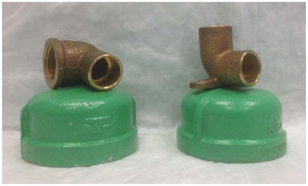
Painted pipe fittings used as novel objects suitable for strong, active mice.

Monitoring behavior—novel object exploration (Day 2)

• 3Transport mice to the testing room and let acclimate for at least 60 minutes.
• 4Turn on recording apparatus.
• 5Place mouse into the center of the open field and allow mice to explore environment, novel objects for 20 min.
• 6During exploration, record all activity by video camera mounted above the open field.
• 7Return mice to holding cage and animal facility when testing is complete.

Scoring behavioral parameters—novel object exploration

• 8Score behavioral parameters in real time or following completion of the task using the video recordings. Parameters include:

  1. Distance traveled (a measure of locomotor activity)

  2. Time spent exploring each object and total object exploration time (a measure of exploratory behavior). Exploration is measured as the time spent contacting or in close proximity to (<2.5 cm) the object but not sitting or perched on the object. If using Ethovison XT, a pre-defined buffer zone can be set around each object so that the boundary is 2.5 cm from all sides of the object. Mice close to the object but facing away from it are not considered to be exploring.

Monitoring behavior—novel object recognition (Day 3)

• 9Readjust open field, video camera, computer monitor and tracking software as necessary if the apparatus was moved.
• 10Place one of the two objects from the previous trial together with one new object of a different type into the open field arena. If multiple testing arenas are being used the position of the novel object should be varied so that it is not always on the same side.
• 11Transport mice to testing room and let acclimate for at least 60 minutes.
• 12Place mouse into the center of the open field and allow mice to explore environment, novel objects for 20 min.
• 13During exploration, record all activity with the video camera mounted above the open field.
• 14Return mice to holding cage and animal facility when testing is complete.

Scoring behavioral parameters—novel object recognition

• 15Score behavioral parameters in real time or following completion of the task using the video recordings. Parameters include:

  1. Distance traveled (a measure of locomotor activity)

  2. Time spent exploring each object and total time spent exploring objects (a measure of recognition memory)

  3. Location of the novel object (left or right side) should be noted so that side preferences can be accounted for.

iii) CONTINUOUS SPONTANEOUS ALTERNATION MAZE

The continuous spontaneous alternation maze is designed to test spatial working memory. A mouse with an intact hippocampus, normal visual acuity and no motor deficits will spontaneously alternate arms of a T- or Y- maze to fully explore its environment. The testing procedure described here does not rely on external motivation or previous experience. To minimize the adverse effects of repeated handling, especially given the variability in ease of restraint in the Diversity Outbred population and wild-derived strains, the continuous alternation version of the task is preferable to repeated trials in which the mouse is moved back to the start arm after each choice.

Materials

• The Med Associates T-maze for mice (St. Albans, VT) T-maze for mice is configured with 14.5″ runways, a square hub (ENV-334U) for the T configuration or a triangular hub (ENV-333U) for the Y configuration, and manually operated guillotine doors (ENV-339U).

• Blue floor inserts (Med Associates, MED-RAMM-BI) to better facilitate video tracking of multiple mouse coat colors.

• Appropriate visual cues (see Prior to starting)

• Video camera hooked to computer monitor

• Real-time video tracking software (e.g., Noldus Ethovision XT)

• Timer

• Holding cage

Prior to starting

• 1The mouse maze must be situated in a room with the appropriate visual cues (i.e., large geometric shapes). In our testing room, two walls contain striking visual cues, including the door wall and a wall with a rack of wire shelving. Prominent visual cues made from dark contact paper are adhered to the unobstructed white walls of the room. These are approximately 18 × 20 inches and cut into a circle and a ‘T’ (Fig. 4).
• 2Mount video camera and synchronize with computer monitor, tracking software.

Figure 4.

Configuration of T-maze and large geometric objects (top, T; bottom, circle).

Monitoring behavior—continuous spontaneous alternation maze (Day 5)

• 3Transport mice to testing room and let acclimate for at least 60 minutes.
• 4Turn on recording apparatus.
• 5Place mice into the enclosed arm of the T-maze and wait 10 seconds.
• 6Lift sliding guillotine door and allow mouse to explore freely for five minutes.
• 7After trial has ended, return mouse to clean duplex home cage with food and water.

Scoring behavioral parameters

• 8Score behavioral parameters in real time or following completion of the task using video recording. Parameters include:

  1. Time spent in each arm (a measure of quality control)

  2. Total distance travelled (a measure of activity)

  3. Number of transitions (a measure of quality control and of exploratory activity). Mice with <2 transitions are excluded from the analysis. In our experience, mice making so few transitions are physically impaired and therefore this assay is unlikely to provide an appropriate estimation of cognitive performance. These mice constitute <1% of the sample in our high-throughput conditions.

  4. Percent of correct alternations (a measure of spatial working memory). Percent of correct alternations is the number of alternations in which the mouse does not repeat either of the previous two arm choices. At each incorrect alternation (e.g., right, left, right), the sequence is reset and a correct alternation cannot be achieved until two non-repeating choices are made (e.g., right, start, left). This can be calculated manually or with the Sequence Analysis Tool macro if using the Ethovision XT software.

iv) TAIL-SUSPENSION TEST

The tail-suspension test places mice in a temporarily inescapable stress situation. The mice initially attempt to escape but eventually cease in an immobility response that is interpreted as learned helplessness or behavioral despair. Shorter durations of immobility or fewer bouts of immobility are thought to indicate a more resilient phenotype. Pharmacological intervention with anti-depressants reduces the time spent immobile.

A potential confound of the test is tail-climbing behavior, which essentially provides an escape. Mice that climb their tails to escape the suspended position will either rest on top of the apparatus and, having discovered this escape, will commonly climb repeatedly throughout the trial. The wild-derived Collaborative Cross and Diversity Outbred progenitor strains climb more than their inbred counterparts (Logan et al., 2013), though the tendency to climb is not limited to outbred or wild-derived strains and is quite common in C57BL/6J mice (Cryan et al., 2005). Subjects that climb must be removed from the immobility analysis. As an alternative, we devised a simple plastic cone (Fig. 5) that is readily cleaned between mice and largely eliminates this confounding behavior.

Figure 5.

Plastic cone to prevent climbing behavior.

Materials

• Horizontal ring-stand bar

• 15 ml polypropylene centrifuge tube, cut to 5.5–6.5 cm long

• Hacksaw

• 640 grit sandpaper or gentle heat source

• Timer

• Holding cage

• Masking tape

• Video camera hooked to computer monitor

• Real-time video tracking software (e.g., Noldus Ethovision XT)

Prior to starting

• 1Prepare the ring-stand bar: a horizontal bar placed approximately 30 cm above the floor of the testing apparatus (see Fig. 6).
• 2Prepare plastic cone:

  1. Using the hacksaw, cut off the top 4–6 cm and bottom 0.4 cm of a 15 ml centrifuge tube. In the Diversity Outbred, we use a variety of lengths to accommodate mice with very short or long tails, a common occurrence in this outbred population.

  2. Remove the burrs from the edges of cut end with 640 grit sandpaper or gentle heat so that no sharp edges remain (Fig. 5).

  3. Note that a cone is used once per mouse then cleaned with 70% ethanol.

• 3Mount video camera appropriately and sync with computer monitor, tracking software.

Figure 6.

Ring-stand bar, height 30cm from floor of testing apparatus to bar.

Monitoring behavior—tail suspension (Day 9)

• 4Transport mice to the testing room and let acclimate for at least 30 minutes. The tail suspension test provides reliable behavioral output with less acclimation time needed than for other tests.
• 5Turn on recording apparatus.
• 6Place plastic cone onto the tail.
• 7Suspend individual mice by a point within the last 2–3 cm from tip of tail on the ring-stand bar and secure using masking tape.
• 8Monitor mice for five minutes.
• 9Return mice to clean duplex home cage with food and water.

Scoring behavioral parameters

• 10Parameters to be measured include:

  1. Duration of immobility (a measure interpreted as behavioral despair). Immobility was quantified using the mobility state variable in Noldus Ethovision XT, which compares the change in pixels from one video frame to the next. We use a sample acquisition rate of 29.9 samples per second, an averaging factor of 1 and a mobility threshold of 5%. These settings were chosen based on the best practices described by Lad et al. 2007, and require optimization for individual laboratories.

  2. The occurrence of climbing behavior. Data from mice that climb are excluded from the analysis. With the use of the plastic tail cone, approximately 1 in 400 mice exhibit this behavior.

Alternate Protocol – Grip Strength as a Measure of Neuromuscular Function

Grip strength is another useful test of aging and might be useful should neuromuscular function be a focus. The grip-strength test assesses the peak amount of force an animal applies when grasping a specially designed pull-bar, and is an indicator of neuromuscular function. Our protocol for grip strength is as follows.

Materials

• Grip-strength meter with digital peak force display (Columbus Instruments, Columbus, OH) (Fig. 7).

• Holding cage

Figure 7.

Grip-strength meter.

Measuring grip strength

1. Transport mice to the testing room and let acclimate for at least 60 minutes prior to testing.

2. Ensure that the grip-strength pull bar is positioned horizontally.

3. Holding mouse by the tail, lower mouse towards the apparatus.

4. Allow mouse to voluntarily grasp the metal pull bar with their forelimbs.

5. Gently pull the mouse backward in the horizontal plane.

6. Record the force applied to the bar at the moment the grasp is released; this is the peak tension (kg).

7. Repeat the test five consecutive times; the highest value from the five trials is recorded as the grip strength for that animal.

8. Return mouse to home cage with food and water after testing.

9. Return all mice to animal facility when testing is complete.

Basic Protocol 3: ASSESSMENT OF KIDNEY FUNCTION

Kidney function is assessed by determining the ratio of microalbumin to creatinine in the urine and the blood urea nitrogen (BUN) levels in serum. Microalbumin does not normally pass through the glomerular membrane; hence, its presence in urine is an indication of kidney damage. Creatinine is a byproduct of muscle metabolism and is normally excreted by urine. The albumin levels are expressed as a ratio to creatinine (albumin-creatinine ratio; ACR) to control for differences in hydration, osmotic diuresis, and concentration (Levey et al., 2005). Elevated BUN also indicates declining kidney function. Specific aspects of kidney function can be assayed by measuring electrolytes, magnesium and glucose levels in the blood. Abnormalities, either high or low, in each of these tests help elucidate any alterations in the function of the kidneys, which serve to maintain the balance of these metabolites.

This assay allows experimenters to collect spot (i.e., single-time-point void) urine for kidney function analyses of microalbumin and creatinine. Freshly voided urine samples are collected in the mornings from individual mice over three days (days 18, 19 and 22 in the cross-sectional study design; see Table 3) and pooled, to ensure sufficient volume of sample for all analyses. Samples are kept at 4°C during pooling and are stable for up to one week (after which freezing is needed). We use the Beckman AU680 Chemistry Analyzer according to the manufacturer’s specifications for these analyses. See Basic Protocol 4 for procedures for obtaining the BUN and for assaying electrolytes, magnesium and glucose levels, which are all measured from plasma samples.

i) URINE COLLECTION

Materials

• Microcentrifuge tubes (1.5mL) for urine collection per animal

• Pasteur pipettes with rubber bulbs

• Weigh boat (one per animal)

Urine Collection using 1.5mL tube

• 1Pick up each mouse gently by scruffing the skin in the cervical region, behind the ears, and securing the head.
• 2Position mouse at appropriate angle so as to allow mouse to void urine freely. For a male mouse, this angle is approximately 60°. For a female mouse, the correct angle is approximately 45°. Proper positioning of the mouse over the microcentrifuge tube is critical to avoid losing urine sample.
• 3If needed, massage bladder gently with thumb by stoking towards legs 5–10 times and allowing urine to fall into tube.

Urine Collection using weigh boat

• 4Pick up mouse gently and position appropriately over weigh boat (as in steps 1–2).
• 5Allow mouse to void freely.
• 6If needed, massage bladder gently (as in step 3).
• 7Allow urine to fall into weigh boat.
• 8Transfer urine to 1.5mL tube with pipette.
• 9If using the Beckman AU680 chemistry analyzer, a minimum volume of 42μL is needed for urine analysis. The Beckman AU680 requires a minimum volume of 20μl of non-tested sample for proper operation, 9μl for the urine microalbumin test and 13μl for the creatinine test. If not all tests are run at once, an additional minimum operational volume is needed for each run.

ii) MEASUREMENT OF MICROALBUMIN CONCENTRATION

Microalbuminuria refers to the increased excretion of albumin in urine. Urine microalbumin levels can be used as a predictive biomarker of diabetic nephropathy and for assessing diabetic complications, as microalbumin tends to present early in urine during renal glomerular damage. This assay is based on an antigen-antibody reaction in which urine samples are combined with an anti-albumin antiserum, forming microalbumin-antibody complexes that scatter light in proportion to their size, shape and concentration. The Beckman Coulter AU680 analyzer measures the reduction in light created by the formation of complexes formed as an increase in absorbance. High absorbance readings indicate high concentrations of microalbumin in the urine. Calibration of the AU680 is done with a traceable albumin standard and is stable for 90 days. The mouse albumin standard dilution should be run at least daily, ideally once per cartridge per day.

Materials

• Chemistry analyzer (i.e., the Beckman Coulter AU680)

• Graphing software (i.e., Excel, GraphPad)

• Mouse albumin (Sigma-Aldrich, Cat. No. A3139)

Materials specific to the AU680

• Goat anti-human albumin antiserum (OSR6167 Beckman Coulter, CA)

• Beckman Protein Diluent (Cat. No. 442825)

• Tris buffer 95 mmol/L (pH 7.6)

• 0.9% saline solution

• Test tubes 12–16mm in diameter or sample cups (Cat. No. AU1063)

• Beckman AU680 Clinical Chemistry Analyzer (Beckman Coulter, CA)

• Beckman Coulter Microalbumin Calibrator (Cat. No. ODR3024)

• Beckman Coulter AU System Microalbumin Reagent (Cat. No. OSR6167)

Establishing a standard curve

• 1Calibrate the chemistry analyzer according to the manufacturer’s recommendations.
• 2Prepare a series of standard mouse albumin concentrations diluted with Beckman Protein Diluent. A series of six standards is typically used (e.g., 25, 12.5, 6.25, 3.125, 1.5625 and 0 mg/dL).
• 3Run these standards for mouse albumin.
• 4Plot known concentrations on x axis and measured values on y-axis using graphing software.
• 5Perform linear regression analysis to obtain slope of the curve. The slope becomes the correction factor for all experimental samples.

Measuring mouse urinary microalbumin concentrations

• 6Load urine samples into your chemistry analyzer, 9μl per sample if using the Beckman AU680.
• 7Determine final urine microalbumin concentration by dividing the measured microalbumin values by the standard slope: [measured microalbumin sample (mg/dL) ÷ standard slope] = actual urine microalbumin concentration (mg/dL).

iii) MEASUREMENT OF CREATININE CONCENTRATION

Measurements of creatinine are used to diagnose renal disease. The Beckman Coulter AU System uses a kinetic procedure modified from the Jaffe procedure (Jaffe, 1886). In this reaction, creatinine reacts with picric acid at alkaline pH to form a yellow-orange complex. The rate of change in absorbance at 520/800nm is proportional to the concentration of creatinine in the sample. For urine, a calibration using a blank (water) and a standard sample should be performed daily. For microalbumin measurements, urine samples may be stored for up to seven days at 2–8°C or up to a year when frozen at ≤−20°C. Creatinine in urine is stable for six days at 2–8°C, and indefinitely at ≤−20°C.

Materials

• Chemistry analyzer (i.e., the Beckman Coulter AU680)

• Graphing software (i.e., Excel, GraphPad)

• Mouse albumin (Sigma-Aldrich, Cat. No. A3139)

Materials specific to AU680

• Sodium hydroxide solution (final concentration 120 mmol/L)

• Picric acid (final concentration 2.9 mmol/L)

• Test tubes 12–16mm in diameter or sample cups (Cat. No. AU1063)

• Beckman AU680 Clinical Chemistry Analyzer (Beckman Coulter, CA)

• Beckman Coulter AU System Creatinine Reagent (Cat. No. OSR6178)

• Beckman Coulter Urine Chemistry Calibrator (Cat. No. DR0091)

Accurate calibration results depend on proper storage of the calibrator, proper use of the AU680 analyzer and proper use of their respective reagents. Discoloration of the reagent or calibrators or visible signs of microbial growth, turbidity or precipitation in the reagent may indicate degradation and warrant discontinuing use of these reagents. Open calibration reagents are stable when refrigerated for up to 90 days.

Measuring mouse urinary creatinine concentrations

1. Ensure that the chemistry analyzer is calibrated to the manufacturer’s specifications.

2. Load urine samples (13μl per sample for the creatinine test) in the calibrated analyzer.

3. Final urine creatinine concentration is reported directly by the analyzer in mg/dL (Grindle et al., 2006).

Interpreting results

Microalbumin readings are reported as the albumin-to-creatinine ratio (ACR) because interpretation requires correction for differences in hydration, osmotic diuresis, and concentration. To obtain the ACR, first correct the albumin values as instructed in step 7, ii) MEASUREMENT OF MICROALBUMIN CONCENTRATION above. Divide the corrected albumin values (mg/dL) by the creatinine values (mg/dL) and multiply this number by 1000 to get the mg/g ACR value.

ACR varies greatly between inbred strains of mice and with age. Normal inbred strains range between non-detectable and ACR values of 200mg/g, although we have seen ACR values in the thousands for certain knockout strains and other animals with known deficiencies in kidney function. In humans, the clinical threshold of 30 mg/g of albumin/creatinine is used as an indicator of potential kidney damage, since increased urinary albumin is one of the first markers of prolonged perturbations in kidney function. Whether this threshold also applies to mice is unclear at the moment. Some strains of mice with high ACR values do not seem to have any histological damage, while at the same time some strains with low ACR do. These could be exceptions due to specific genetic variations. More research on larger populations and more inbred strains is needed to determine a threshold for mice.

For the microalbumin assay, the AU680 analyzer is linear from 0.5–30 mg/dL. Samples exceeding the upper limit of linearity should be diluted and repeated. For the creatinine assay, the picric acid-creatinine reaction is not completely specific for creatinine since other reducing substances (e.g., glucose, pyruvate, ascorbic acid, and acetoacetates) will react with picrate to form a similar color. It is known that the Jaffe method is not useable for mouse serum (Grindle et al., 2006). Because of the problems in using the Jaffe method in mouse serum, creatinine clearance measures are not routinely used in mice as a measure of kidney function.

Basic protocol 4: BLOOD COLLECTION FOR ASSESSMENT OF HEMATOLOGICAL, IMMUNOLOGICAL AND METABOLIC PARAMETERS

In this protocol, we describe our method for collecting blood and measuring individual blood parameters. Mice are fasted for four hours (i.e., from 7:30 to 11:30 am for an 11:30 am collection) before they are bled via the retro-orbital sinus or via submandibular cheek puncture. Each blood collection consists of three individual collections spaced two weeks apart and centered around six, 12, and 18 months of age to enable the comprehensive measurement of a variety of hematological, immunological and metabolic parameters. In collection 1, the serum is isolated and used to measure basic electrolyte levels (sodium, potassium), magnesium, blood urea nitrogen (a measure of kidney function) and glucose (a measure of metabolic regulation). In collection 2, EDTA-anticoagulated whole blood is processed to obtain complete blood counts (CBC), including cell differentials and reticulocyte counts; this enables the detection of anemia and, when combined with other parameters, the source can often be deduced (e.g., anemia from renal dysfunction, anemia from inflammation, bone marrow failure). Collection 3 is split several ways to enable assessment of cytokines (i.e., IGF1) by ELISA and immune cell counts by flow cytometry. Over the three aforementioned ages, the comprehensive data provided enable detailed analysis of the changes in blood, immune and metabolic function in aging.

BLOOD COLLECTION 1

Collection of serum for blood chemistry analysis of:

• Blood Urea Nitrogen (BUN, mg/dL)

• Basic Electrolytes: (Sodium (mmol/L), Potassium (mmol/L)

• Magnesium (mg/dL)

• Glucose

Materials

• Yellow-capped Microtainer® tube with serum separator, one for each mouse (BD, Cat. No. 365967)

• 1.5mL collecting tubes, labeled, for each mouse

• Heparinized capillary tubes

• Tray for holding serum tubes

• Tray for holding 1.5mL tubes

• Ice in a container

• Weight scale

Preparation on day of procedure

• 1Remove food from cages four hours in advance of blood collection. For strains that shred their grain onto the floor of their cages, it may be necessary to move the mice to a clean cage for the duration of the fasting period.
• 2Mark mice to be bled beforehand.
• 3Transport mice to the procedure room to acclimate within 60 minutes of the procedure.
• 4Label yellow serum tubes for as many mice as are needed.
• 5Remove “pouring” cap from each tube, to be replaced with the yellow cap after bleeding.
• 6Mark up 1.5mL collection tubes for as many mice as are needed.
• 7Weigh each mouse and record weight on spreadsheet.

Bleeding of mice

• 8Bleed mice via the retro-orbital sinus or submandibular cheek puncture into a labeled yellow serum tube; about 200μL should be sufficient. The final volume needed will depend on which chemistry analyzer to be used. With the Beckman AU680, a full panel of renal metabolites requires 83μl of serum. Requirements are 20μl of dead volume, 21μl for the BUN (run in triplicate), 28μl for electrolytes, 7μl for magnesium and 7μl for glucose.
• 9Replace yellow plug cap onto tube and place tube on ice.
• 10Return the mouse to its cage and provide food and water as per normal for that caging system.
• 11Return the cage to its normal spot in the animal holding room.
• 12Centrifuge all samples at 18,000g for 10 minutes at 4°C. Timing is critical to minimize hemolysis between blood draw and centrifugation.
• 13Remove the plug caps from each tube.
• 14Reapply the pouring caps to each tube and pour serum into the corresponding clean 1.5 ml tube.
• 15Place the serum in either the refrigerator or on the bench top if the sample will be tested promptly, or place at −20°C if the testing of the samples will not be conducted for days or weeks (see below for sample storage information for the various assays).
• 16Dispose of serum tubes containing the whole pellet.

i) MEASUREMENT OF BLOOD UREA NITROGEN FROM SERUM

Blood urea nitrogen (BUN) levels can be used to assess renal function and failure. Urea nitrogen comprises approximately 75% of total non-protein nitrogen in blood, and is synthesized in the liver from ammonia as a product of protein deamination. Surplus nitrogen is eliminated from the body mainly through filtration of urea from the blood into the urine by the renal glomeruli. Renal causes of increased BUN include acute glomerulonephritis, chronic nephritis, polycystic kidney disease, nephrosclerosis and tubular necrosis.

We use the Beckman Coulter AU680 Analyzer for measuring BUN, which uses a method whereby urea is hydrolyzed by urease to yield ammonia and carbon dioxide. L-glutamate dehydrogenase (GLDH) catalyzes the conversion of ammonia and α-oxoglutarate to glutamate, while, simultaneously, a molar equivalent of reduced NADH is oxidized. The rate of change in absorbance at 340 nm is directly proportional to the BUN concentration in serum and results from the disappearance of NADH. Serum samples for BUN analysis are stable for up to 24 hours at room temperature (15–25°C), several days at 2–8°C, and 2–3 months at ≤−20°C. Calibration of BUN on the Beckman AU680 should be done when reagent lots are changed, and quality control with known standards should be performed daily.

Materials- Specific to AU680

• Test tubes 12–16mm in diameter or sample cups (Cat. No. AU1063)

• Beckman AU680 Clinical Chemistry Analyzer (Beckman Coulter, CA)

• Beckman Coulter Chemistry Calibrator (Cat. No. DR0070)

• Beckman Coulter AU System Urea (BUN) Nitrogen Reagent (Cat. No. OSR6134/6234)

Measuring mouse serum BUN concentrations

1. Calibrate the analyzer according to the manufacturer’s specifications.

2. Load serum samples into Analyzer (7μl for BUN).

3. If using the AU680, run the test in triplicate.

4. Results are automatically printed for each sample in mg/dL.

Interpreting results

Expected ranges for BUN in inbred mice range from 10.7–34.2 mg/dL.

ii) MEASURING BASIC ELECTROLYTES (Na+, K+) FROM SERUM

Electrolytes perform a variety of critical metabolic and physiological functions. They maintain osmotic pressure and hydration of various body fluid compartments as well as proper body pH, regulate heart and muscle function and participate in a variety of enzyme reactions. Electrolytes are measured from serum using the Beckman Coulter AU680 Analyzer. Crown ether membrane electrodes specific for Na+ and K+ are used to assess electrical potential. When compared to the internal reference solution, this electrical potential is translated into voltage and then into the ion concentration of the sample. Multipoint calibration of the machine is to be performed daily. Use fresh samples for analysis wherever possible, although Na+ and K+ are stable in serum for at least one week at 2–8°C in stoppered tubes.

Materials-Specific to AU680

• Test tubes 12–16mm in diameter or sample cups (Cat. No. AU1063)

• Beckman AU680 Clinical Chemistry Analyzer (Beckman Coulter, CA)

• Beckman Electrodes: Na⁺ Electrode (Cat No. MU9194), K⁺ Electrode (Cat No. MU9195) and Reference Electrode (Cat No. MU9197)

• Beckman ISE Buffer (Cat No. AUH1011)

• Beckman ISE Reference Solution (Cat No. AUH1013)

Accurate calibration results depend on proper storage of calibrator, proper technique the use of the AU680 analyzer, and in their respective reagents. Discoloration of reagent or calibrators, visible signs of microbial growth, turbidity or precipitation in the reagent may indicate degradation and warrant discontinuing the use of these reagents. Open calibration reagents are stable when refrigerated for up to 90 days.

Measuring mouse serum electrolyte concentrations

1. Calibrate analyzer according to the manufacturer’s specifications.

2. Load serum sample (28μL) into the analyzer.

3. Individual electrolyte concentrations are given in mEq/L at 37°C.

Interpreting results

Expected ranges for Na+ and K+ in mice are 129–188 mmol/L and 5.85–9.74mmol/L respectively.

For the serum Na+ assay, the AU680 analyzer is linear from 50–200 mEq/L. For the serum K+ assay, the AU680 analyzer is linear from 1.0–10.0mEq/L. Samples exceeding the dynamic range of the assay should be diluted with deionized water and re-assayed. The results obtained must be multiplied by the dilution factor to obtain the correct concentration for the undiluted sample.

According to the technical documents provided by the AU680 manufacturer, electrolyte determinations may be affected by the presence of certain coagulants, preservatives, drugs and organophilic compounds. Visually turbid urine samples should be centrifuged prior to analysis.

iii) MEASURING MAGNESIUM LEVELS FROM SERUM

Magnesium is a major intracellular cation that activates a number of important enzyme systems engaged in the transfer and hydrolysis of phosphate groups. Decreased serum magnesium levels have been observed in diabetes, thyroid disease, malabsorption, myocardial infarction and other conditions of aging, while increased serum magnesium can be seen in renal failure, severe diabetic acidosis and other conditions. Magnesium is measured in the Beckman Coulter AU680 analyzer using a direct method in which magnesium forms a colored complex with xylidyl blue in a strongly basic solution. The color produced is measured bichromatically at 520/800 nm and is proportional to the magnesium concentration. Magnesium in serum is stable for one week stored at 2–8°C. A calibration using a blank (water) and a standard sample (the Beckman Coulter AU System Creatinine Reagent) should be performed daily.

Materials specific to the AU680

• Test tubes 12–16mm in diameter or sample cups (Cat. No. AU1063)

• Beckman AU680 Clinical Chemistry Analyzer (Beckman Coulter, CA)

• Beckman Coulter Chemistry Calibrator (Cat. No. DR0070)

• Beckman Coulter AU System Magnesium Reagent (Cat. No. OSR6189)

Measuring mouse serum magnesium concentrations

1. Calibrate analyzer according to the manufacturer’s specifications.

2. Load serum samples into the analyzer (7 μl for magnesium).

3. Results are automatically printed for each sample in mg/dL. Results in mg/dL can be divided by 1.21 to obtain mEq/L.

Interpreting results

According to the mouse phenome database (http://phenome.jax.org/) expected ranges for Mg++ are 1.9–2.7 mg/dL.

iv) MEASUREMENT OF GLUCOSE FROM SERUM

Glucose metabolism is a vital indicator of health, and suboptimal glucose levels are commonly observed in aging, particularly in the context of type 2 diabetes. We use the Beckman Coulter AU680 analyzer to measure glucose concentration from serum according to a timed-endpoint method, in which hexokinase catalyzes the transfer of a phosphate group from ATP to glucose. This leads to the formation of ADP and glucose-6-phosphate (G6P). G6P is then oxidized to 6-phosphogluconate with the concomitant reduction of NAD to NADH by G6P dehydrogenase. The change in absorbance at 340nm is directly proportional to the concentration of glucose in the sample. The AU680 system should be calibrated every 30 days and precision-checked daily. However, a hand-held glucose meter may be used in place of the AU680 depending on the study protocol. Use of this is described in Blood Collection 3.

Materials specific to AU680

• Test tubes 12–16mm in diameter or sample cups (Cat. No. AU1063)

• Beckman AU680 Clinical Chemistry Analyzer (Beckman Coulter, CA)

• Beckman Coulter Chemistry Calibrator (Cat. No. DR0070)

• Beckman Coulter AU System Glucose Reagent (Cat. No. OSR2161)

Measuring mouse urinary creatinine concentrations

1. Calibrate analyzer according to the manufacturer’s specifications.

2. Load serum samples into the analyzer (7 μl for glucose).

3. Results are automatically printed for each sample in mg/dL.

Interpreting results

Expected ranges for blood glucose are 100–500 mg/dL and 150–200 mg/dL for fasted glucose. Strain and within strain sex differences exist for most phenotypes, including glucose, and can be found on the Mouse Phenome Database.

BLOOD COLLECTION 2

Collection of whole blood for complete blood cell counts, differentials and reticulocyte counts. A small amount of plasma is also stored for future assays. Unlike chemistry tests discussed above which require serum, EDTA-anticoagulated whole blood is required for complete blood counts to prevent clotting.

Materials

• Siemens ADVIA 2120 Hematology Analyzer equipped with mouse-specific software (see Notes below)

• Microhematocrit tubes: EDTA-coated, 75 mm, 75 μL volume size (Fisherbrand®)

• Blood collection tubes: Microtainer® tube containing lyophilized K₂EDTA (Becton-Dickinson Diagnostics, Franklin Lakes, NJ or Fisher Catalogue #36-5974)

• Second set of 1.5mL tubes for collecting plasma, labeled

• Pipetteman able to accommodate 100 μl of blood

• Pipette tips

• Trays for holding tubes

• Ice in a container

• Standard body weight scale

Preparation on day of procedure

• 1Remove food from cages four hours in advance of blood collection.
• 2Mark mice to be bled beforehand.
• 3Transport mice to procedure room to acclimate within one hour of the procedure.
• 4On the day of the bleed, mark EDTA tubes for each mouse, as well as the 1.5mL tubes.
• 5Set out tubes in two holding trays, as well as toothpicks and pipette tips.
• 6Label the 1.5mL tubes for the collection of plasma.
• 7Scan mice to verify identity.
• 8Weigh each mouse and record weight on spreadsheet.

Bleeding of mice

• 9Collect 270 μL of blood (about 13 drops plus one capillary tube) via retro-orbital bleeding or submandibular cheek puncture using an EDTA-coated capillary tube directly into a BD Microtainer tube coated with lyophilized K₂EDTA. (Note: If plasma is not needed, the amount of blood drawn can be reduced to 170 μL).
• 10Invert the tube to mix (do not vortex).
• 11Insert a wooden toothpick to determine if any clots are present, which will cling to the toothpick and be visible. Micro-clots will clog the analyzer. If anything larger than a micro-clot is present, accuracy of counts will be compromised and the sample should therefore be discarded.
• 12Aliquot 100 μL of whole blood into the corresponding 1.5mL collection tube.
• 17Place EDTA tube into the holder at room temperature (and use within 3h; otherwise, refrigerate and bring to room temperature prior to hematology analysis).
• 18Place 1.5mL tube on ice.
• 19Repeat for all mice.

Storage of serum for future assays

• 20Spin down the 1.5 mL collecting tubes for 10 minutes at 4°C.
• 21Remove 35–40 μL of plasma from each tube and aliquot into the corresponding plasma collection tube.
• 22Store samples at −80°C.

Blood cell count with differential using Siemens Advia 2120 system

• 23Analyze blood using the Seimens ADVIA 2120 system according to the manufacturer’s protocol.
• 24Select CBC/DIFF/RETIC to obtain the following measurements:

  1. White blood cell count (WBC),

  2. Red blood cell count (RBC),

  3. Hemoglobin (HGB),

  4. Hematocrit (HCT),

  5. Mean corpuscular volume (MCV),

  6. Mean corpuscular hemoglobin (MCH),

  7. Mean corpuscular hemoglobin content (MCHC),

  8. Differential count (% neutrophil, % lymphocytes, % monocytes, % eosinophils, LUCs),

  9. Platelet (PLT) count,

  10. % reticulocytes (Retic),

  11. Platelet count.

These are the basic parameters of a CBC. Depending upon the exact analyzer used, other parameters may also be available. For example, the Siemens Advia 2120 includes the RDW (red cell distribution width), HDW (hemoglobin distribution width), and MPV (mean platelet volume). The CBC is a rapid screen for many diseases arising from a lack of one (e.g., anemia, thrombocytopenia, neutropenia) or multiple (pancytopenia) cell types as well as diseases arising from an over-production of certain cell lineage(s) (i.e., leukemia). Although there are many differences in the absolute numbers of cells in mice versus humans, their relationships to disease are similar. For example, normal mouse RBC counts are much higher and the RBC volume (MCV) much smaller than in humans. Despite this, when mouse RBC numbers and sizes are decreased compared to a proper control of the same inbred strain, one can confidently diagnose anemia. Thus, because humans and mice get the same diseases, a basic clinical hematology text such as Henry’s (McPherson et al., 2011) is a valuable tool for interpreting the mouse CBC. Texts devoted to mouse hematology are also available (see chapter 5, Fox et al., 2007; McGarry et al., 2009). CBC data for >30 inbred mouse strains at ages up to 18–24 months are available on the Mouse Phenome Database (phenome.jax.org).

Complete blood counts (CBC) with differential and reticulocytes can be obtained using any standard hematology analyzer. In our program, we use the Siemens Advia 2120 Hematology Analyzer equipped with mouse-specific software. It is important to ensure the hematology analyzer is programmed using mouse-specific hematological settings. The size of red and other blood cells in mouse is smaller than in humans and different relative to other species. Therefore, the use of non-mouse parameters will significantly affect the results. Obviously, it is critical that blood analyzers are calibrated according to the manufacturer’s specifications and that appropriate controls are run appropriately for quality assurance.

BLOOD COLLECTION 3

This collection is split three ways, with an instant read of plasma glucose also being measured: For flow cytometry, as with the CBC, anticoagulated whole blood is required.

1. 65μL is collected as plasma and banked for experiment-specific assays such as ELISAs for serum cytokines or other or hormones. These assays are not described here.

2. 15μL plasma is saved for IGF1 measurements, which is measured by ELISA according to the instructions provided with the assay kit (Mouse/Rat IGF-I Quantikine ELISA Kit, MG100, R&D Systems).

3. The cell pellet left after spinning down the samples is analyzed with flow cytometry using standard surface markers of immune cells. This assay (adapted from Petkova et al., 2008) is described below.

Materials

• Microhematocrit tubes: heparinized, 75 mm, 75 μL volume size (Fisherbrand®)

• Blood collection tubes: Microtainer® tube containing lyophilized K₂EDTA (Becton-Dickinson Diagnostics, Franklin Lakes, NJ or Fisher Catalogue #36-5974)

• Second set of 1.5mL tubes for collecting plasma, labeled

• Pipetteman able to accommodate 100 μL of blood

• Pipette tips

• Trays for holding tubes

• Ice in a container

• Standard body weight scale

• Glucose Reader

• Glucose Strips

• Centrifuge

Flow cytometer (Beckton Dickinson (BD) FACScan (BD Biosciences, San Jose, CA) with 5-color upgrade (Cytek Development, Fremont, CA), or FACS Calibur (BD Biosciences, San Jose, CA)) Parafilm© all-purpose laboratory film

• 200 μL and 1000 μL pipette tips (USA Scientific, Ocala, FL)

• 12 × 75 mm polypropylene (USA Scientific 1450-0000FC)

• 0.9% phosphate-buffered saline (PBS)

• Hemolytic Geys buffer (see Julius and Herzenberg, 1974)

• FACS Buffer (PBS with 2 mM EDTA, 0.02% NaN3, and 2% FBS)

• FlowJo software (TreeStar, Inc., Ashland, OR)

• Propidium iodide 20 μg/mL solution in FACS buffer for dead cell exclusion

Antibody cocktail for B cells and myeloid cells (purchased from e-Biosciences, San Diego, CA or PharMingen, San Diego, CA):

• CD45R/B220—Pacific Blue clone RA3-6B2

• Gr-1—APC-Cy7 clone RB6-8C5

• CD11c—FITC clone N418

• CD11b/Mac-1—PE clone M1/70

• F4/80—AlexaFluor 647

*Antibody cocktail for T cells and NK cells:

• CD3e—PE clone 145-2C11

• CD4—APC clone RM 4-5

• CD8—AlexaFluor 700 clone 53-6.7

• CD44—APC-Cy7 clone IM7.8.1

• CD62L—PE-Cy7 clone MEL-14

• NKG2A/C/E—FITC clone 20d5

• B220—Pacific Blue.

NOTE: All antibodies should be titrated to determine optimal staining levels with minimum background staining for the conditions specific to your laboratory. The specified monoclonal antibody clones have not been tested on all strains. It is possible the antibodies do not recognize all isotypes of the marker. Thus, low cell numbers for a population might not be a good reflection of the actual count.

Preparation on day of procedure

• 1Remove food from cages four hours in advance of blood collection. (Note: This is important if glucose determinations are to be made, and possibly for certain hormone determinations. It is not necessary if only IGF1 will be assayed or for flow cytometry.) A 4–6 hour fast is common for determinations of blood glucose levels (Kebede et al, 2014; Svenson et al 2007), although variations are many. For example, IMPReSS (International Mouse Phenotyping Resource of Standardised Screens) does not fast at all for simple blood glucose determinations, but fasts overnight for a glucose tolerance test (details at https://www.mousephenotype.org/impress).
• 2Mark blood collection tubes for each mouse, as well as 1.5mL tubes for plasma.

Bleeding of mice and glucose measurement

• 3Remove a single mouse cage from the cage rack and place cage in a controlled air-flow hood or in the procedure room.
• 4Verify identity.
• 5Weigh each mouse and record weight on the spreadsheet.
• 6Collect 200 μL of whole blood (about six drops plus one capillary tube) via a retro-orbital or submandibular bleed, using a heparin-coated capillary tube, directly into a BD Microtainer tube coated with lyophilized K₂EDTA.
• 7Place tube on ice.
• 8Use the remaining blood in the capillary tube to dab onto glucose strip to get glucose reading.
• 9Record glucose value on the spreadsheet.

Handling of plasma, pellet samples

• 10Centrifuge tubes at 500g for five minutes at 4°C to separate cells from plasma.
• 11Aliquot plasma into the 1.5 mL polypropylene tubes for each sample. Store at −20°C to −80°C.
• 12Following removal of the plasma, resuspend the cell pellet in 200 μL FACS buffer and transfer to 12 × 75 mm polypropylene tubes.

Preparation of pellet for flow cytometry

• 13Add 3 mL hemolytic Geys solution to each polypropylene tube and incubate for five minutes at room temperature.
• 14Centrifuge tubes at 500g for five minutes to separate the hemolyzed red blood cells.
• 15Decant the hemolyzed red cell and buffer layer.
• 16Resuspend the pelleted cells in an additional 3 mL of Geys buffer and incubate for 3–5 min at room temperature, and then centrifuge again at 500g.
• 17Decant the wash buffer and resuspend the pelleted cells in 4 mL FACS buffer.
• 18Aliquot cells into three new 12 × 75 mm tubes and centrifuge at 500g for five minutes.
• 19Decant the supernatant layer and resuspend each tube of pelleted cells in 100 μL of FACS buffer with the appropriate fluorescently labeled antibodies.

Fluorescence labeling_and flow cytometry analysis of peripheral blood cell counts

• 20Add 10μL of antibody cocktail at the proper dilution to each sample. Mix the sample well and incubate on ice for 30 min to allow the cells to stain.
• 21Wash stained cells by adding 2 mL of FACS buffer to each tube and then centrifuging at 500g for five minutes at 4°C.
• 22Decant the supernatant and resuspend the pellet in 250 μL of FACS buffer.
• 23Add 10 μL of propidium iodide using a 20 μg/mL stock solution for identification of dead cells.

Flow cytometry analysis of peripheral blood cell counts

• 24Acquire cell counts on the BD FACScan (with Cytek 5 color upgrade) cytometer or the BD FACS Calibur according to the manufacturer’s protocol.
• 25Analyze the acquired cell count files with FlowJo software (TreeStar, Inc., Ashland, OR).

  1. Viable cells are gated by forward scatter channel (FSC) and exclusion of propidium iodide. Red blood cells are also excluded as they have lower FSC than lymphocytes.

  2. Lymphocytes are gated from the viable cells by FSC versus sides scatter channel (SSC) for T cells, B cells, and natural killer (NK) cells.

  3. B cells are gated from the lymphocytes as positive for the CD45R/B220 antigen (B220+ cells).

  4. T cells are gated from the lymphocyte gate on the basis of CD3 and CD4 expression for CD4+ T cells (T helper cells), and CD3 and CD8 expression for CD8+ T cells (cytotoxic T cells).

  5. CD4+ and CD8+ T-cell subsets are gated for CD44 and CD62L. The memory and naive cells are defined as: CD44 high, CD62L low (effector memory), CD44 high, CD62L high (central memory), CD44 low, CD62L low, and CD44 low, CD62L high (naive).

  6. NK cells are reported as CD3-, NKG2A/C/E+.

  7. Granulocytes are gated as CD11b+, Gr-1 high, and SSC high.

  8. Eosinophils are gated as Gr-1 mid to low, SSC very high, and CD11b mid to high.

  9. Monocytes are gated as CD11b-positive and SSC low (as compared to granulocytes).

  10. Inflammatory monocytes are gated as CD11b-positive, CD11c-negative, Gr-1 mid.

  11. Resident monocytes are gated as CD11b-positive, CD11c-positive, Gr-1-negative cells.

• 26Report the data for each cell subpopulation as the percentage of total viable cells. T-cell subsets are also reported as a percentage of total T cells.

Basic Protocol 5: ASSESSMENT OF SKELETAL AND BODY COMPOSITION

With aging, alterations in weight, muscle mass and body composition are common and often predictive of health status. For example, weight loss is strongly predictive of mortality, an association that appears to be independent of disease (Newman et al., 2005). Age-related reduction in lean muscle mass leads to fatigue, decreased strength, poor balance and increased risk of injury. Finally, decreased adult bone mineral density is an important risk factor for bone fracture, the risk of which increases significantly with age. Dual-energy X-ray absorptiometry (DXA) is the standard method for determining in vivo body composition in humans and is used clinically for diagnostic purposes for certain bone diseases such as osteoporosis. Here, we describe our DXA protocol using the PIXImusII mouse densitometer, an electrically driven dual-energy X-ray machine (Nagy and Clair, 2000). This machine allows us to measure total body areal bone mineral density, lean mass and fat mass with high sensitivity in living animals, and is therefore suitable for longitudinal and/or cross-sectional studies.

Materials

• LUNAR PIXImusII mouse densitometer (DXA; GE-Lunar)

• Tribromoethanol 2% (w/v) or other suitable anesthetic (check with the institution’s rules and recommendations for selecting an anesthetic for small animals for non-surgical procedures.)

• Standard weight scale

• Hypodermic needles and syringes

• Imaging tray to hold the mouse on the instrument (purchased specifically for use with the PIXImus instrument)

• Exogenous heat source for recovery from anesthesia, such as a water-circulating warming pad or a slide warmer placed under the cage

Method for animal handling and restraint

• 1Place mice in clean cages and bring to location of the PIXImusII.
• 2Weigh each mouse and anesthetize appropriately. [*Gwen to add cross-ref]
• 3Wait until the mouse is completely anesthetized as any movement of the mouse during the scan will invalidate the result.

Procedure for collecting body composition scan

• 4Place mouse on the plastic imaging tray and scan immediately following the instructions for the PIXImusII instrument. A single scan takes approximately five minutes to complete.

  1. Position the mouse carefully for imaging. The mouse must be placed ventral side down and the limbs arranged such that all four paws are placed flat against the imaging tray and are visible when viewing the mouse from above.

  2. Place the tail such that it too is on the imaging tray and is NOT left to extend off of the back of the tray.

  3. Ensure that the entire mouse (exclusive of the head) fits on the adhesive part of the imaging tray.

  4. Ensure that no part of the mouse (excluding head) is outside of this adhesive region as this the area that will be imaged. It is crucial that the whole body be imaged for accurate data collection and for valid comparisons between mice.

• 5At end of the scan, remove mice and allow to recover from anesthesia under an exogenous heat source.
• 6Return mice to original mouse room.
• 7Use the software to exclude the head region from the image. Apply any Regions of Interest (ROI) filters following the instructions in the PIXImusII user manual and export the data for further analysis.

Interpretation of data

The DXA provides three basic types of information: lean, fat and mineralized tissue mass. From these three values, all other measures made by the PIXImus are calculated. The values exported by the PIXImus are presented in Table 5.

Table 5.

Values exported by the PIXImusII

Measure	Units	Notes
Bone area	cm2	The total area of the mouse that was interpreted as mineralized tissue, looking down on the mouse from above.
Bone mineral content (BMC)	g	The calculated amount of mineral present in the whole mouse (exclusive of the head) or in the ROI.
Bone mineral density (BMD)	g/cm2	Calculated by dividing BMC by bone area and, as such, is an animal size–corrected parameter.
Total area	cm2	The projected area of the mouse looking down from above.
Ratio of soft tissue attenuation coefficients		This value is not used for small animal studies usually. This value is unitless.
Percent fat	%	The calculated amount of fat present in the whole mouse (exclusive of the head) divided by the total tissue mass of the mouse. Total fat mass is calculated by the machine, but not presented in the standard export function. It can be back-calculated from this exported value.
Total tissue mass (TTM)	g	This is the estimated bodyweight of the mouse and is calculated by summing BMC, total fat mass and total lean mass.
Total lean mass	g	The calculated amount of lean mass present in the whole mouse. Total lean mass is calculated by the machine, but not presented in the standard export function. It can be back-calculated using exported values. This value is presented on the output screen at the time of scan analysis.

Notes

Total tissue mass (TTM) should correlate strongly with the body weight of the mouse, as measured with a standard balance. That said, as the head is excluded from the TTM value, this value is usually approximately 1 g less than traditional whole mouse body weight.

Subcutaneous microchips and metal ear tags used for mouse identification may not be compatible with DXA analysis. The microchips, while usually implanted in the scapular region, will migrate around the mouse and months after implant can be found almost anywhere subcutaneously on the dorsal side of the mouse. As the microchips are X-ray-opaque, the microchip will be erroneously interpreted as mineral by the PIXImus software. As these migrate around the mouse, it is not a simple matter of simply excluding the microchip from the area imaged as different part of the mouse will be excluded each time. Metal ear tags that are small can be used as long as these are completely excluded with the head region during analysis of the image.

Gaseous anesthetics are usually administered to a mouse via a nose cone. These nose cones are often too large to be practically excluded with the head during the analysis and as such their use should be avoided.

The PIXImus takes a series of four images per mouse and each scanning cycle takes approximately one minute to complete. These four images are aggregated together for data collection. If the mouse moves during scanning, multiple “images” of the mouse will be collected, leading to artifacts in the data.

Basic Protocol 6: MORPHOLOGICAL EYE ANALYSIS

This protocol describes methods for assessing eye morphology, with an emphasis on cataracts, by slit-lamp ophthalmoscopy. Pupils are dilated using an anticholinergic solution to facilitate examination of cataracts and eye morphology.

Materials

• Slit-lamp biomicroscope (e.g., Nikon NS-1 Slit Lamp)

• Pupillary dilation solution (e.g., 1% Atropine Sulfate Ophthalmic Solution (sterile), Alcon

• Laboratories, or 1% Cyclopentolate Hydrochloride Ophthalmic Solution USP (sterile), Bausch & Lomb)

Procedure

1. Transport mouse to testing room and let acclimate for five minutes.

2. Restrain and hold the mouse firmly in one hand.

3. Adjust the light emitted from the slit lamp and shine the light into the mouse eye (Fig. 8).

4. Examine the cornea for clarity, size (buphthalmos versus microcornea), surface texture, and vascularization.

5. Examine the iris for pupillary size and central location, iris constriction when exposed to bright light, reflected luminescence and synechia (adhesion to the cornea or lens).

6. Dilate the eye using 1% atropine by placing one drop into one eye.

7. Once eye is dilated, use slit lamp to examine pupil for cataracts.

Figure 8.

A–B: Slit lamp biomicroscope for the examination of the anterior segment (i.e. iris, cornea, lens) of the eye. C–D: Close-up of the light source (green asterisk) of slit-lamp in A–B.

Notes: Morphological alterations of the cornea include, but are not limited to, changes in the normal transparency of the cornea (i.e., cloudy cornea, white cornea/corneal opacity); presence of corneal scarring (i.e., corneal spot) or fibrosis and neovascularization (i.e., corneal vessels); and signs of corneal trauma (i.e., corneal tear). Severity can be described as diffuse or focal (small, medium, and/or large spot). See examples in Fig. 9. Other alterations in the normal transparency of the cornea (i.e., diffusely hazy, cloudy or white corneas, focal spots) may be observed (Fig. 8). These can be congenital, infectious, traumatic or idiopathic in origin.

Figure 9.

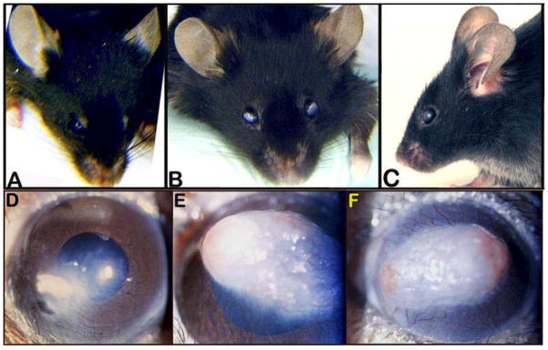
A: Superficial gross appearance of the normal eye and cornea. B and C: Superficial gross appearance of a bilateral corneal change in transparency. D: Small spot with peripheral cloudy appearance of the cornea. E: Large white spot with signs of neovascularization in the cornea. F: Diffusely white cornea with neovascularization and two foci of corneal ulcerations.

Morphological alterations of the lens include, but are not limited to, cataract formations originating from the lens nucleus or lens sutures (Fig. 10), aberrant adhesions of the lens to the cornea (i.e., corneal-lens synechia), abnormal lens location, and alteration of the overall transparency of the lens fibers (i.e., lens haze, lens snowflakes, lens spots). Fig. 9 shows a healthy dilated eye and lens along with examples of snowflake, nuclear or suture cataracts.

Figure 10.

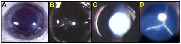
A: Fully dilated eye showing normal, clear and transparent, lens. B: An example of lens snowflake cataract. C: An example of a lens nuclear cataract. D: An example of a lens suture cataract.

COMMENTARY

Background information

In 2000, the Mouse Phenome Project (MPP) was proposed (Paigen and Eppig, 2000). The result has been an explosion of large-scale phenotyping in an ever-expanding repertoire of mouse populations. Prior to the initiation of the MPP, high throughput, comprehensive phenotyping in mice was largely limited to directed ENU (N-ethyl-N-nitrosourea) mutagenesis screens in a single mouse strain. The MPP succeeded in changing the scale of discovery such that systematic phenotyping was performed, in many cases, on > 30 strains including inbred, recombinant inbred, consomic, congenic, and knockout strains of mice. The Mouse Phenome (http://phenome.jax.org/), the IMPC (International Mouse Phenotyping Consortium, http://www.mousephenotype.org/), the German Mouse Clinic (http://www.mouseclinic.de/), and the European Mouse Disease Clinic (EUMODIC, www.europhenome.org) databases, to name just a few, are now populated with extensive phenotype data for laboratory mice.

Not unexpectedly, the application of high throughput phenotyping to aging mouse populations has followed; the Mouse Phenome Database is populated with multiple studies devoted to lifespan and the effects of aging on a wide range of biological disciplines (e.g., bone biology, chromosomal stability, hearing, hematology). In addition, a large ENU screen to uncover novel phenotypes in aging mice is underway (Goldsworthy and Potter, 2014). Phenotype-driven studies in defined strains of mice make it possible to uncover novel phenotype-genotype relationships and gene-environment influences in aging mouse populations.

Critical Parameters

Methods of euthanasia for gene expression and other post-mortem analyses and rationale for use

Projects that incorporate post-mortem analyses will need to consider the method of euthanasia to be used. While CO₂ asphyxiation is a well-accepted and common form of euthanasia, it is inappropriate for use in gene-expression, metabolic or proteomic studies from whole blood as this form of euthanasia results in hypoxia-induced changes in gene expression. For these types of studies, sera/tissues need to be free of anesthetics, diluents, gases or treatment-induced changes in the animal’s physiology. Two suitable alternatives that we use are cervical dislocation and decapitation, the latter of which is an ideal method for collecting large quantities of blood.

Rationale for food and water restrictions

When tissue will be collected for gene expression, or when blood will be collected for the purpose of measuring a factor affected by recent food intake (i.e., serum glucose levels), the mice are deprived of food for four hours prior to euthanasia or blood collection. This is necessary to minimize short-term changes in gene expression in the tissues of interest that would directly result from the consumption and digestion of food. Likewise, many factors in blood spike quickly after food consumption. Deprivation of food for four hours allows for a “wash out” of changes in blood factors and/or gene expression changes that are directly associated with immediate consumption of food.

Although a 4–6 hour fast is common for glucose determinations, overnight fasts of up to 16 hours are used as well. In our experience with aging mice, however, an overnight fast can be detrimental to aged mice, particularly in those strains that are small, have low baseline glucose to start with or are otherwise frail.

Definition of moribund: when to terminate life in studies of aging

To understand why mice must be allowed to live their full lifespans in the study of aging, consider that living creatures, mice and humans, are assemblies of biological systems, all working together at different levels—molecular, subcellular, cellular, tissue and organ. Lifespan is determined by the first biological system to fail beyond compensation. This has vital implications for studies of basic mechanisms of aging. Such mechanisms are rarely if ever involved in diseases and forms of damage that reduce lifespans, since only one system must fail to cause death in those instances.

By contrast, an increase in lifespan requires that no biological systems fail over a longer period of time. This is most likely to occur when the basic mechanisms of aging are altered, since these mechanisms affect many different biological systems. We do not yet know what such mechanisms are, but only that they exist. For these reasons, the gold standard for assessing the basic mechanisms of aging, particularly the genetic regulation of aging, is increased lifespan. To obtain a true measure of maximum lifespan we must not stress animals, but allow them to live as long as they can. We therefore must not euthanize animals until we are certain that they would die if we did not interfere.

After much experience with aging mice, and after extensive consultation with other members of the aging research community outside of The Jackson Laboratory, we have determined that the only reliable signs of terminal decline, i.e., moribund, are the following five symptoms:

1. Lack of response to touch or other stimuli.

2. Labored breathing.

3. Cold to the touch.

4. Hunched body posture with matted fur.

5. Signs of sudden weight loss, failure to eat/drink, prominent protrusion of ribs and spine, and sunken hips.

Rapid weight loss is defined as loss of 20% of body weight within six days; however, this measure is more accurate in large mice. Mice showing any of the other criteria listed above (AD) should be weighed every three days to assess rapid weight loss, and observed daily. Weighing the mice more frequently is stressful for older mice (and for the cage mates) and should be avoided. For small mice, prominent protrusion of ribs and spine and sunken hips may be evident before 20% of the animal’s weight is lost. If the spine or ribs become grossly apparent over the course of four days of observation, this will be considered “sudden weight loss” when determining the condition of moribund.

In our experience, the presence of these five criteria is required to define a mouse as truly moribund and, therefore, a single measure is not sufficient for all strains. For example, we recognize that “not responsive to touch” is a valid single endpoint for many strains. However, it is an insufficient criterion in mice that normally do not respond to touch, such as obese mice and some diabetic strains of mice. Furthermore, for studies using de novo knockout lines, it may not be clear from the outset what pathologies will develop over the course of their lifespan, making it impossible to be sure that “not responsive to touch” will be a valid endpoint to define a moribund state. This is why it is essential to incorporate additional criteria. When all these criteria are present, mice will die soon, and can be euthanized. Obviously even with these criteria, the people judging if an aging mouse is moribund must have experience with that population and must follow enough mice through natural death to be able to tell when the mouse is truly moribund, versus when a mouse has a good chance of recovery.

Troubleshooting

Instrumentation and sample procurement/processing

Problems in phenotyping (e.g. extreme outlier values) most commonly result from inappropriately maintained and/or calibrated equipment, inaccurately obtained or processed samples or inexperienced personnel. Effective phenotyping using sophisticated instruments such as the Beckman AU680 Clinical Chemistry Analyzer requires knowledge of the instrumentation being used, its sample requirements and limitations, common errors encountered and troubleshooting protocols. A detailed discussion of each instrument’s specific operating requirements is beyond the scope of this discussion. However, manufacturer literature provides a wealth of information on these topics. Moreover, for the use of advanced instruments, it is always prudent to attend training workshops, which are commonly offered by their manufacturers.

Technician variability

In our experience it is critical to develop “experts” for each phenotyping assay and to have the expert perform the assay in each animal at all time points, to the extent possible. All technical personnel have their strengths and weaknesses, and variations in technique add to variations in results.

Diurnal effects

Diurnal variations affect laboratory test results and are particularly important in glucose, white blood cell and hormone determinations, among many others. Hence, it is critical that any given test be performed at the same time of day.

Anticipated Results

The overall goals of long-term lifespan and health-span studies vary tremendously. Thus, only broad generalizations of anticipated results are helpful. Statistical analysis of the effects of an intervention (e.g., caloric restriction, effects of a gene knockout, inbred strain background effects) on lifespan is straightforward (Yuan et al., 2009, 2012). However, interpretation of health-span status depends on the parameters tested, as clearly not every tissue and organ system can be assayed directly. The pipeline described here was designed to give a broad systems view of the effects of aging in multiple physiological areas that reflect the interests and expertise of those involved; that can be done in tandem while preserving the integrity of each test; that fit within practical constraints such as budget; and that, most importantly, reflects current, compelling issues and problems in humans aging (e.g., cognitive decline, anxiety, declining physical strength, age-related disease).

Time Considerations

Longitudinal and cross-sectional studies of lifespan and health-span in mice represent an enormous commitment of resources. The most important time consideration is the overall pipeline. Our strategy was designed to phenotype a total of 600 mice (300 male, 300 females) centered around three time points (Table 3). By spreading the phenotyping “window” over 25 days, as well as by planned breeding to produce mice in cohorts for phenotyping, it was possible to include a large number of phenotyping assays in the pipeline. Thus, the pipeline was tailored to accommodate the desired phenotypes in a fashion that did not overwhelm available resources of time, budget and personnel.

References

- Ackert-Bicknell CL, Karasik D, Li Q, Smith RV, Hsu YH, Churchill GA, Paigen BJ, Tsaih SW. Mouse BMD quantitative trait loci show improved concordance with human genome wide association loci when recalculated on a new, common mouse genetic map. J Bone Miner Res. 2010;25:1808–1820. doi: 10.1002/jbmr.72. [DOI] [PMC free article] [PubMed] [Google Scholar]
- Chesler EJ, Wilson SG, Lariviere WR, Rodriguez-Zas SL, Mogil JS. Identification and ranking of genetic and laboratory environment factors influencing a behavioral trait, thermal nociception, via computational analysis of a large data archive. Neurosci Biobehav Rev. 2002;26(8):907–923. doi: 10.1016/s0149-7634(02)00103-3. [DOI] [PubMed] [Google Scholar]
- Cryan JF, Mombereau C, Vassout A. The tail suspension test as a model for assessing antidepressant activity: Review of pharmacological and genetic studies in mice. Neurosci Biobehav Rev. 2005;29(4–5):571–625. doi: 10.1016/j.neubiorev.2005.03.009. [DOI] [PubMed] [Google Scholar]
- Deacon RMJ, Rawlins JNP. T-maze alternation in the rodent. Nature Protocols. 2006;1:7–12. doi: 10.1038/nprot.2006.2. [DOI] [PubMed] [Google Scholar]
- Ennaceur A, Delacour J. A new one-trial test for neurobiological studies of memory in rats. 1: Behavioral data. Behav Brain Res. 1988;31(1):47–59. doi: 10.1016/0166-4328(88)90157-x. [DOI] [PubMed] [Google Scholar]
- Fitzmaurice Garrett, Davidian Marie, Verbeke Geert, Molenberghs Geert., editors. Longitudinal Data Analysis. Boca Raton, FL: Chapman and Hall/CRC; 2008. [Google Scholar]
- Fox JG, Barthold S, Davisson M, Newcomer CE, Quimby FW, Smith A, editors. The Mouse in Biomedical Research. 2. Academic Press, Inc; San Diego: 2007. pp. 566–567. [Google Scholar]
- Gerlai R. A new continuous alternation task in T-maze detects hippocampal dysfunction in mice. A strain comparison and lesion study. Behav Brain Res. 1998;95(1):91–101. doi: 10.1016/s0166-4328(97)00214-3. [DOI] [PubMed] [Google Scholar]
- Goldsworthy ME, Potter PK. Modelling age-related metabolic disorders in the mouse. Mamm Genome. 2014;25:487–496. doi: 10.1007/s00335-014-9539-6. [DOI] [PMC free article] [PubMed] [Google Scholar]
- Grindle S, Garganta C, Sheehan S, Paigen B, DiPetrillo K. Validation of High-throughput methods for measuring blood urea nitrogen and urinary albumin concentrations in mice. Comp Med. 2006;56(6):482–6. [PubMed] [Google Scholar]
- Jaffe MZ. Ueber den Niederschlag welchen Pikrinsäure in normalen Harn erzeugt und über eine neue reaction des Kreatinins. Z Physiol Chem. 1886;10:391–400. [Google Scholar]
- Julius MH, Herzenberg LA. Isolation of antigen-binding cells from unprimed mice: demonstration of antibody-forming cell precursor activity and correlation between precursor and secreted antibody avidities. J Exp Med. 1974;140(4):904–920. doi: 10.1084/jem.140.4.904. [DOI] [PMC free article] [PubMed] [Google Scholar]
- Kebede MA, Oler AT, Gregg T, Balloon AJ, Johnson A, Mitok K, Rabaglia M, Schueler K, Stapleton D, Thorstenson C, Wrighton L, Floyd BJ, Richards O, Raines S, Eliceiri K, Seidah NG, Rhodes C, Keller MP, Coon JL, Audhya A, Attie AD. SORCS1 is necessary for normal insulin secretory granule biogenesis in metabolically stressed β cells. J Clin Invest. 2014;124:4240–4256. doi: 10.1172/JCI74072. [DOI] [PMC free article] [PubMed] [Google Scholar]
- Kenyon CJ. The genetics of ageing. Nature. 2010;464:504–512. doi: 10.1038/nature08980. [DOI] [PubMed] [Google Scholar]
- Levey AS, Eckardt KU, Tsukamoto Y, Levin A, Coresh J, Rossert J, Zeeuw D, Hostetter TH, Lameire N, Eknoyan G. Definition and classification of chronic kidney disease: a position statement from Kidney Disease: Improving Global Outcomes (KDIGO) Kidney Int. 2005;67:2089–2100. doi: 10.1111/j.1523-1755.2005.00365.x. [DOI] [PubMed] [Google Scholar]
- Lad HV, Liu L, Paya-Cano JL, Fernandes C, Schalkwyk LC. Quantitative traits for the tail suspension test: automation, optimization, and BXD RI mapping. Mammalian Genome. 2007;18(6–7):482–491. doi: 10.1007/s00335-007-9029-1. [DOI] [PMC free article] [PubMed] [Google Scholar]
- Leduc MS, Hageman RS, Meng Q, Verdugo RA, Tsaih SW, Churchill GA, Paigen B, Yuan R. Identification of genetic determinants of IGF-1 levels and longevity among mouse inbred strains. Aging Cell. 2010;9:823–836. doi: 10.1111/j.1474-9726.2010.00612.x. [DOI] [PMC free article] [PubMed] [Google Scholar]
- Logan RW, Robledo RF, Recla JM, Philip VM, Bubier JA, Jay JJ, Harwood C, Wilcox T, Gatti DM, Bult CJ, Churchill GA, Chesler EJ. High-precision genetic mapping of behavioral traits in the diversity outbred mouse population. Genes Brain Behav. 2013;12(4):424–37. doi: 10.1111/gbb.12029. [DOI] [PMC free article] [PubMed] [Google Scholar]
- McGarry MP, Protheroe CA, Lee JJ. Mouse Hematology: A Laboratory Manual. Cold Spring Harbor Laboratory Press; New York: 2009. [Google Scholar]
- McPherson RA, Pincus MR. Henry’s Clinical Diagnosis and Management by Laboratory Methods. 22. Elsevier (Saunders); Philadelphia, PA: 2011. [Google Scholar]
- Milsom I, Coyne KS, Nicholson S, Kvasz M, Chen CI, Wein AJ. Global Prevalence and Economic Burden of Urgency Urinary Incontinence: A Systematic Review. European Urology. 2014;65(1):79–95. doi: 10.1016/j.eururo.2013.08.031. [DOI] [PubMed] [Google Scholar]
- Murabito JM, Yuan R, Lunetta KL. The search for longevity and healthy aging genes: insights from epidemiological studies and samples of long-lived individuals. The Journals of Gerontology Series A, Biological Sciences and Medical Sciences. 2012;67:470–479. doi: 10.1093/gerona/gls089. [DOI] [PMC free article] [PubMed] [Google Scholar]
- Murray EA, Bussey TJ, Saksida LM. Visual perception and memory: a new view of medial temporal lobe function in primates and rodents. Annu Rev Neurosci. 2007;30:99–122. doi: 10.1146/annurev.neuro.29.051605.113046. [DOI] [PubMed] [Google Scholar]
- Nagy TR, Clair AL. Precision and accuracy of dual-energy X-ray absorptiometry for determining in vivo body composition of mice. Obesity Res. 2000;8:392–398. doi: 10.1038/oby.2000.47. [DOI] [PubMed] [Google Scholar]
- Natalin R, Lorenzetti F, Dambros M. Management of OAB in Those Over Age 65. Current Urology Reports. 2013;14(5):379–385. doi: 10.1007/s11934-013-0338-5. [DOI] [PubMed] [Google Scholar]
- Newman AB, Lee JS, Visser M, Goodpaster BH, Kritchevsky SB, Tylavsky FA, Nevitt M, Harris TB. Weight change and the conservation of lean mass in old age: the Health, Aging and Body Composition Study. Am J Clin Nutr. 2005;82:872–878. doi: 10.1093/ajcn/82.4.872. [DOI] [PubMed] [Google Scholar]
- Oeppen J, Vaupel JW. Demography. Broken limits to life expectancy. Science. 2002;296:1029–1031. doi: 10.1126/science.1069675. [DOI] [PubMed] [Google Scholar]
- Petkova SB, Yuan R, Tsaih SW, Schott W, Roopenian DC, Paigen B. Genetic influence on immune phenotype revealed strain-specific variations in peripheral blood lineages. Physiological Genomics. 2008;34:304–314. doi: 10.1152/physiolgenomics.00185.2007. [DOI] [PMC free article] [PubMed] [Google Scholar]
- Royce JR. On the construct validity of open-field measures. Psychological Bulletin. 1977;84(6):1098–1106. [Google Scholar]
- Sinke AP, Caputo C, Tsaih SW, Yuan R, Ren D, Deen PM, Korstanje R. Genetic analysis of mouse strains with variable serum sodium concentrations identifies the Nalcn sodium channel as a novel player in osmoregulation. Physiological Genomics. 2011;43:265–270. doi: 10.1152/physiolgenomics.00188.2010. [DOI] [PMC free article] [PubMed] [Google Scholar]
- Svenson KL, Smith RV, Magnani PA, Suetin HR, Paigen B, Naggert JK, Li R, Churchill GA, Peters LL. Multiple trait measurements in 43 inbred mouse strains capture the phenotypic diversity characteristic of human populations. J Appl Physiol. 2007;102:2369–2378. doi: 10.1152/japplphysiol.01077.2006. [DOI] [PubMed] [Google Scholar]
- Tikkinen KA, Agarwal A, Griebling TL. Epidemiology of male urinary incontinence. Current opinion in Urology. 2013;23(6):502–508. doi: 10.1097/MOU.0b013e328364f520. [DOI] [PubMed] [Google Scholar]
- Walsh RN, Cummins RA. The open-field test: a critical review. Psychological Bulletin. 1976;83(3):482–504. [PubMed] [Google Scholar]
- Wimmer ME, Hernandez PJ, Blackwell J, Abel T. Aging impairs hippocampus-dependent long-term memory for object location in mice. Neurobiol Aging. 2012;33(9):2220–4. doi: 10.1016/j.neurobiolaging.2011.07.007. [DOI] [PMC free article] [PubMed] [Google Scholar]
- Wooley CM, Xing S, Burgess RW, Cox GA, Seburn KL. Age, experience and genetic background influence treadmill walking in mice. Physiology & Behavior. 2009;96:350–361. doi: 10.1016/j.physbeh.2008.10.020. [DOI] [PMC free article] [PubMed] [Google Scholar]
- Xing S, Tsaih SW, Yuan R, Svenson KL, Jorgenson LM, So M, Paigen BJ, Korstanje R. Genetic influence on electrocardiogram time intervals and heart rate in aging mice. American Journal of Physiology Heart and Circulatory Physiology. 2009;296:H1907–1913. doi: 10.1152/ajpheart.00681.2008. [DOI] [PMC free article] [PubMed] [Google Scholar]
- Yu W, Ackert-Bicknell C, Larigakis JD, MacIver B, Steers WD, Churchill GA, Hill WG, Zeidel ML. Spontaneous voiding by mice reveals strain-specific lower urinary tract infection to be a quantitative genetic trait. Am J Physiol Renal Physiol. 2014;306(11):F1296–1307. doi: 10.1152/ajprenal.00074.2014. [DOI] [PMC free article] [PubMed] [Google Scholar]
- Yuan R, Tsaih SW, Petkova SB, Marin de Evsikova C, Xing S, Marion MA, Bogue MA, Mills KD, Peters LL, Bult CJ, Rosen CJ, Sundberg JP, Harrison DE, Churchill GA, Paigen B. Aging in inbred strains of mice: study design and interim report on median lifespans and circulating IGF1 levels. Aging Cell. 2009;8:277–287. doi: 10.1111/j.1474-9726.2009.00478.x. [DOI] [PMC free article] [PubMed] [Google Scholar]
- Yuan R, Peters LL, Paigen B. Mice as a mammalian model for research on the genetics of aging. ILAR. 2011;52:4–15. doi: 10.1093/ilar.52.1.4. [DOI] [PMC free article] [PubMed] [Google Scholar]
- Yuan R, Meng Q, Nautiyal J, Flurkey K, Tsaih SW, Krier R, Parker MG, Harrison DE, Paigen B. Genetic coregulation of age of female sexual maturation and lifespan through circulating IGF1 among inbred mouse strains. Proc Natl Acad Sci USA. 2012;109:8224–8229. doi: 10.1073/pnas.1121113109. [DOI] [PMC free article] [PubMed] [Google Scholar]