Abstract
Background
When a drug is applied on the skin surface, the concentration of the drug accumulated in the skin and the amount of the drug eliminated into the blood vessel depend on the value of a parameter, r. The values of r depend on the amount of diffusion and the normalized skin-capillary clearence. It is defined as the ratio of the steady-state drug concentration at the skin-capillary boundary to that at the skin-surface in one-dimensional models. The present paper studies the effect of the parameter values, when the region of contact of the skin with the drug, is a line segment on the skin surface.
Methods
Though a simple one-dimensional model is often useful to describe percutaneous drug absorption, it may be better represented by multi-dimensional models. A two-dimensional mathematical model is developed for percutaneous absorption of a drug, which may be used when the diffusion of the drug in the direction parallel to the skin surface must be examined, as well as in the direction into the skin, examined in one-dimensional models. This model consists of a linear second-order parabolic equation with appropriate initial conditions and boundary conditions. These boundary conditions are of Dirichlet type, Neumann type or Robin type. A finite-difference method which maintains second-order accuracy in space along the boundary, is developed to solve the parabolic equation. Extrapolation in time is applied to improve the accuracy in time. Solution of the parabolic equation gives the concentration of the drug in the skin at a given time.
Results
Simulation of the numerical methods described is carried out with various values of the parameter r. The illustrations are given in the form of figures.
Conclusion
Based on the values of r, conclusions are drawn about (1) the flow rate of the drug, (2) the flux and the cumulative amount of drug eliminated into the receptor cell, (3) the steady-state value of the flux, (4) the time to reach the steady-state value of the flux and (5) the optimal value of r, which gives the maximum absorption of the drug. The paper gives valuable information which can be obtained by this two-dimensional model, that cannot be obtained with one-dimensional models. Thus this model improves upon the much simpler one-dimensional models. Some future directions of the work based on this model and the one-dimensional non-linear models that exist in the literature, are also discussed.
Background
A non-linear dual-sorption model of percutaneous drug absorption is described in [2]. Another mathematical model of percutaneous drug absorption and its exact solution is described in [3]. In [4], the non-linear percutaneous permeation kinetics of timolol is studied in vitro with human cadaver skin. A model for a suspension with a finite dissolution rate is solved numerically in [5]. In [6], a mathematical model is developed for percutaneous drug absorption with regular applications of the drug. All these models are one-dimensional and the region of contact of the skin with the drug, is a single point, say x = 0, where x measures the distance into the skin.
To the authors' knowledge, no two-dimensional mathematical model of percutaneous drug absorption exists in the literature, where the region of contact is a line segment, say x = 0, 0 ≤ y ≤ Lc. The purpose of this paper is to model the above situation mathematically and to obtain an efficient finite-difference method to solve it numerically. The usual loss of accuracy along the boundary, where the boundary conditions are of mixed type, is dealt with in a novel approach.
Methods
Model equations
It is an established fact that the stratum corneum, viable epidermis and upper dermis have distinctly different transport and partitioning characteristics, and diffusion through the dermis could be a critical determinant of the percutaneous absorption profiles at least for some kinds of drugs. The model is developed based on the classical view that a drug molecule is rapidly removed by the capillary once it is partitioned into the dermis. Therefore, the skin-capillary boundary may be, anatomically, interpreted as the stratum corneum-dermis boundary.
Let the drug be applied as an ointment on the skin-surface, say, {(0, y) : 0 ≤ y ≤ Lc}, at time t = 0. Let the thickness (distance between the skin-surface and skin-capillary boundary) of the skin be unity. Assuming that skin is an isotropic medium, that is, the diffusivity is the same in the x and y directions, the concentration c(x, y, t) of the drug is given by Fick's Second Law of Diffusion, namely
![]()
where Ld, Lu and Lc are positive real numbers. Assuming that the concentration at the uppermost epidermis {(0, y, t) : 0 ≤ y ≤ Lc} is maintained at unity, the boundary conditions for the model are given by
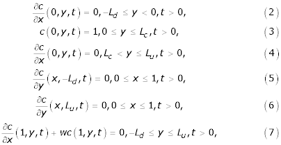
where  .
.
In the above notation, kc is the normalized skin-capillary clearence, kd is the diffusion parameter and r is the concentration at the skin-capillary boundary when the concentration at the uppermost epidermis is regarded as unity (see [3]). Assuming that there is no drug in the skin before the application, the initial distribution associated with the PDE is
c(x, y, 0) = 0, 0 ≤ x ≤ 1, -Ld ≤ y ≤ Lu (8)
The flux J = J(t), through the skin to the receptor site, per unit area, is given by
![]()
(Fick's First Law of Diffusion), so that, from (7),
![]()
The cumulative amount of drug eliminated into the receptor cell per unit area at time τ (see [2]) is
![]()
Numerical methods
The approach to be adopted in obtaining a numerical solution, is the method of lines in which the initial/boundary-value problem to be solved is transformed into a first-order initial-value problem. The region associated with the skin is given by Rs = {(x, y, t) 0 ≤ x ≤ 1, -Ld ≤ y ≤ Lu, t > 0}. Let N be a positive integer, and H = 1/(N + 1). Also it is assumed that Lc = QCH, Lu = QuH, Ld = QdH, where Qc, Qu and Qd are positive integers. Superimpose on Rs a square grid with mesh length H > 0 and let k > 0 be a constant time step. The grid points are given by (xl, ym, tj); xl = lH, l = 0(1)(N + 1), ym = mH, m = -Qd(1)Qu and tj = jk, j = 0,1,2,.... The finite-difference solution which approximates the solution c(x, y, t) of the two-dimensional parabolic equation (1), is sought at each mesh point (xl, ym, tj) in the region [Rs-{0, y), 0 ≤ y ≤ Lc}] × t > 0. For notational simplicity, denote
![]()
At any time-level  or
or  , the {(Qd+ Qu + 1)(N + 2) - (Qc + 1)} elements will be ordered in rows parallel to the x-axis and in vector form, and will be denoted by C(t) and Q, where Q is due to the boundary conditions and is independent of time. For W = C and Q, and
  or
or  , denote

In the above notation n takes the value 0 if m ≠ 0(1)Qc and takes the value 1 otherwise. The vector C(t) is a vector of unknowns and Q is given by by  , for m = 0(1)Qc . All other
  are zero. In the following discretizations, (xl, ym) and cl,m, respectively, denote (xl,ym,tj) and
  . At any time-level t = tj, the differential equation (1) can be discretized as
![]()
If  and
and  are respectively, suitable approximations to cxx;l,m, and cyy;l,m, the above discretization can be written as
![]()
Discretization at (x0, ym), m = -Qd:-
![]()
The boundary condition (5) gives c0,m-1 = c0,m+1. Discretizing the boundary condition (2) gives c-1,m = c1,m Substituting these values of c0,m-1 and c-1,m in (13) gives
![]()
The above equation can be written in the form
![]()
where
![]()
Discretization at (x0, ym), l = 1(1) N, m = -Qd:- Using the boundary condition (5), the required discretization is
![]()
where
![]()
Discretization at (x0, ym), m = -Qd + 1, -Qd + 2,...., -2, Qc + 2, Qc + 3,.., Qu -1:- Using the the boundary conditions (2) and (4), the required discretization is
![]()
where
![]()
Discretization at (x0, ym), m = -1:- Using the boundary conditions (2) and (3), the required discretization is
![]()
where
![]()
Discretization at (x1, ym), m = 0,1,....,Qc:- Using the boundary condition (3), the required discretization is
![]()
where
![]()
Discretization at (x0, ym), m = Qc + 1:- Using the boundary conditions (3) and (4), the required discretization is
![]()
where
![]()
Discretization at (xl, ym), m = Qu:- Using the boundary conditions (2) and (6), the required discretization is
![]()
where
![]()
Discretization at (xl, ym), l = 1(1)N, m = Qu:- Using the boundary condition (6), the required discretization is
![]()
where
![]()
Discretization along the boundary x = 1, -Ld <= y <= Lu.
At the grid point (xN+1, ym) the differential equation (1) can be written as
![]()
Let
cxx;N+1,m = αcN,m + βcN+1,m + γcxxx;N+1,m (24)
Using the Taylor-series expansion for CN,m about the point (xN+1, ym) in (24), and then equating the constant terms, and the coefficients of cxx;N+1,m and cxxx;N+1,m, gives
α = 2/H2, β = -2(1 + Hw)/H2, γ = H/3. (25)
Differentiating (1) with respect to x and (7) with respect to y and t, respectively, and then using the assumptions cxyy;N+1,m = cyyx;N+1,m and cxt;N+1,m = ctx;N+1,m, an expression for cxxx;N+1,m is obtained as
cxxx;N+1,m = -wct;N+1,m + wcyy;N+1,m (26)
Substituting (25) and (26) in (24) gives
cxx;N+1m = αcN,m + βcN+1,m + γ{-wct;N+1,m + cyy;N+1,m} (27)
Substituting (27) in (23) and then replacing ctN+1,m by  and using the approximation
  in the resulting equation, the required difference scheme along the boundary x = 1 is
![]()
where

At an interior grid point (xl, ym), the parabolic equation (1) is discretized as
![]()
where
![]()
Combining the discretizations (15) to (22), (28) and (29), a system of ordinary differential equations is formed as
![]()
where
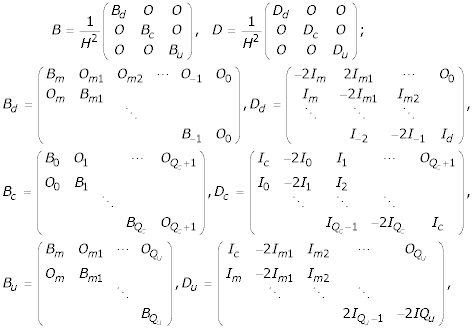
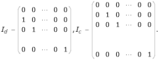
The value of m in Bd and Dd is -Qd, and that in Bu and Du is Qc + 1. The abbreviations m1, m2, ... etc. represent m + 1, m + 2, ... etc. The matrices Id and Ic are square matrices of order N + 1 and N + 2 respectively and are given by
For m = 0,1,2,...,Qc, Bm, are square matrices of order N + 1 and each is given by

For m ≠ 0,1,2,...,Qc, Bm are square matrices of order N + 2 and each is given by

For m = 0,1,...,Qc, Im and Om are the unit square matrix and zero matrix of order N + 1. For m ≠ 0,1,2,...Qc, Im and Om are the unit matrix and zero matrix of order N + 2. Solving the system of ordinary differential equations given by (30), subject to the initial condition(8), gives
C(t) = et(B+D) Q - (B + D)-1Q; (31)
which satisfies the recurrence relation
C (t + k) = ek(B+D) C(t) + (B + D)-1 ek(B+D) Q - (B + D)-1 Q. (32)
To obtain numerical solutions C(t + k), Padé approximants to the matrix exponential ek(B+D) may be used in (32). A fully implicit method may be developed by first writing (32) in the form
C(t + k) = ekD ekBC(t) + (B + D)-1 ekD ekB Q - (B + D)-1 Q; (33)
which has O(k2) error in time. Equation (33) may be approximated further, also with error O(k2), by introducing the (1,0) Padé approximants to the matrix exponential functions ekD, ekB and writing (33) in the split form
(I - kB)C* = C(t) + C+, (34)
(I - kD)C(t + k) = C* - (I - kD)C+.
where the vector C+ is independent of time and is calculated from the equation
(B + D)C+ = Q.
This fully implicit algorithm defined by (34) is first-order accurate in time and second order accurate in space, and is L0-stable. The accuracy in time is improved by extrapolating, as in Lawson and Morris [7]. Let C0, C1 and C2, defined by (35), (36) and (37), respectively, be the three approximations to the solution of (30) at time level t + 2k. The Lawson-Morris algorithm takes the form
(I - kB)C* = C(t) + C+,
(I - kD)C(t + k) = C* - (I - kD)C+,
(I - kD)C** = C(t + k),
(I - kB)C0 (t + 2k) = C** - (I - kB)C+. (35)
(I - 2kB)C* = C(t) + C+,
(I - 2kD)C1 (t + 2k) = C* - (I - 2kD)C+. (36)
(I - 2kD)C* = C(t + 2k) + C+,
(I - 2kB)C2 (t + 2k) = C* - (I - 2kB)C+. (37)
Then the linear combination of these three schemes (35), (36) and (37) defined by
![]()
is second-order accurate in time. That is, the first-order methods (35), (36) and (37) have been extrapolated to achieve second-order accuracy.
The values of the flux J(tj) and the cumulative amount of the drug eliminated into the receptor cell per unit area Ae(tj), at any time-level t = tj = jk, j = 0,1,2, ....etc, are calculated using the trapezoidal rule to approximate the integrals in (10) and (11). Thus, for second-order accuracy,
![]()
and
![]()
Results and discussion
In order to examine the behaviour of the extrapolation method, a number of experiments, similar to those in one space dimension described in [3], are carried out for two space dimensions. The parameter r was given the values 0.00001, 0.0001, 0.001, 0.2, 0.4, 0.6 and 0.8. The space step h was given the value 0.1 so that N = 9 and the time step k is put equal to 0.001. Also, Lc = 0.5, Lu = 3 and Ld = 2.5 so that Qc = 5, Qu = 30 and Qd = 25.
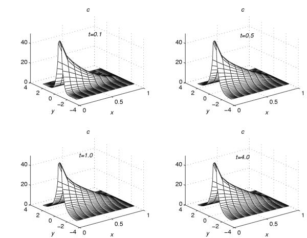
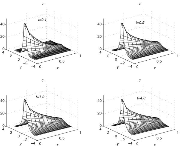
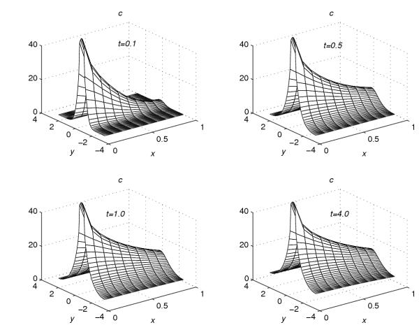
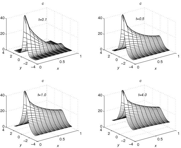
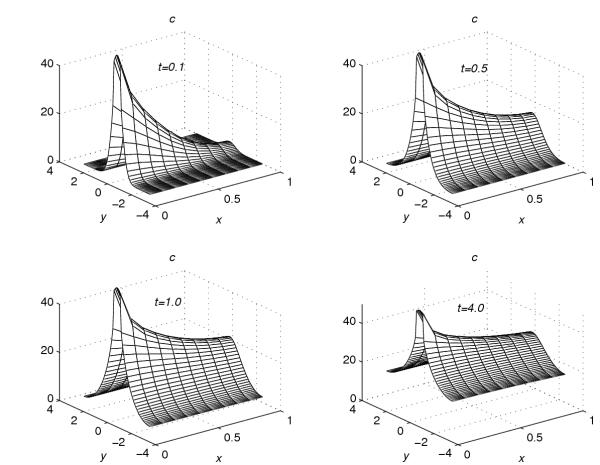
Using the extrapolation technique (38), corresponding to each value of r = 0.001, 0.2, 0.4, 0.6 and 0.8, the concentration profiles at t = 0.1, t = 0.5, t = 1.0 and t = 4.0 are given in Figures 1, 2, 3, 4, 5. These graphs show the effect of the value of the parameter r on the accumulation of the drug into the skin region.
Figure 1.
Concentration profiles for r = 0.001
Figure 2.
Concentration profiles for r = 0.2
Figure 3.
Concentration profiles for r = 0.4
Figure 4.
Concentration profiles for r = 0.6
Figure 5.
Concentration profiles for r = 0.8
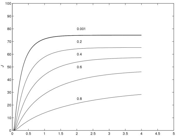
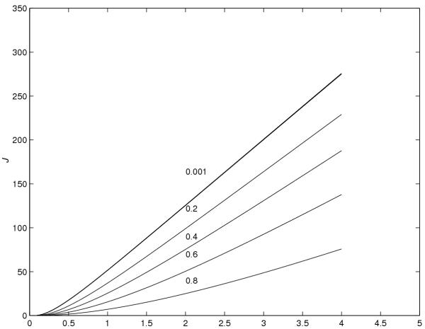
Using the trapezoidal rule given in (39) and (40), the graphs of J versus time and Ae versus time, respectively, are plotted in Figures 6 and 7. These graphs show the effect of the value of r on the the flux and the cumulative amount of drug eliminated into the receptor cell.
Figure 6.
J versus time for various values of r
Figure 7.
Ae versus time for various values of r
Some authors prefer to retain the dimensions of quantities, but the full range of information can be given in a simple manner when dimensions are eliminated. The authors believe that, for this particular study, it is more appropriate not to use dimensions.
Conclusion
The value of r is not easy to control and the major features relating to it include lipophilicity and the molecular weight of the drug. Various drugs with various lipophilicity and molecular weight will have different r-values, so that the profiles will be different between drugs. The value of r will be just one of the factors in selecting the best drug and best vehicle (ointment) design. Various values of r have been used to illustrate what will be predicted by the model. Based on the profiles given, the following conclusions are drawn.
From Figures 1, 2, 3, 4, 5, the following conclusions are made.
(1) For any value of r, the flow rate towards the skin-capillary boundary is larger than the flow rate near to the skin surface. (2) For larger values of r, the difference between the concentration near to the skin surface and the concentration near to the skin-capillary boundary decreases at a faster rate, compared to smaller values of r.
From Figures 6 and 7, however, the following conclusions are made.
(1) As the value of r increases, the flux and the cumulative amount of drug eliminated into the receptor cell, at a particular time, decrease. (2) As the value of r decreases, the steady-state value of the flux increases. (3) The time required to reach the steady-state value of the flux is smaller for smaller values of r. (4) To the scale used, the graphs for r = 0.00001, 0.0001 and 0.001 were found to be coincident, and it is concluded that the value of r = 0.001 is the optimal value of r which gives the maximum absorption of the drug into the blood stream.
The skin has a complicated structure while the model presented is simple. Though the complicacy itself does not always preclude the successful use of a simple model, if the major assumptions made in this model do not hold, what will be observed may differ from what the model predicts. For example, as to the x-axis, the skin consists of stratum corneum and dermis. The use of a simple model for the x-direction may be warranted because the major barrier is normally assumed to be provided by the stratum corneum, [1].
Considering the diffusion of a drug, however, where the diffusion through dermis is a critical component, the y-directional diffusion of drug molecules through the dermis may also be important and what is observed will be different from what the model in this study predicts. The model presented in this study may therefore be used to examine the mechanism of diffusion in the y-direction.
As shown in the non-linear model in [2], which assumes that the drug molecules are either dissolved (mobile) or immobile inside the skin, the drug permeation profiles are considerably different from those described in the linear model. In this study, it was shown that the drug permeation described by the two-dimensional linear model is different from that by the one-dimensional linear model. The percutaneous drug absorption described by a non-linear two-dimensional model will be studied in future work and further comparison based on [2] will then be warranted.
The mathematical model considered in this paper does not take into account the complex, in vivo physiology of skin. The model is developed by simplifying (or ignoring some complexity of) the skin structure. Several models in the literature, used to describe the kinetic behaviour of a drug, have in fact made this simplification. These models do not give any insight into the drug kinetics at the site distant from the area where the ointment is directly applied. As the title of this paper suggests, the model described has taken into account the above issue in the form of y-directional diffusion. That is, the time-course of the drug concentration (which may be best measured in an in vitro study), at the site distant from the area where the ointment is directly applied, is examined in the present paper. No attempt has been made to relate the model to experimental data, because the authors have no access to experimental data which can be related to the two-dimensional model, where the issue of the y-directional diffusion is examined. The authors hope that publication of this model will stimulate researchers to carry out relevant experimental studies, based on diffusion in the direction parallel to the skin surface.
This two-dimensional model improves upon the much simpler models in one-dimension, by giving information of the time-course of drug kinetics in the skin, where the ointment is not directly applied, assuming that the process can be described by a simple homogeneous membrane. If what is observed is different from what this model describes, this may give some clue to elucidate the mechanism of y-directional diffusion of the drug (for example, the diffusivity in the stratum corneum may be different between x- and y- directions or the y-directional diffusion through the dermis, once it is permeated through the stratum corneum, may change). Those features cannot be known from one-dimensional models.
Authors' Contributions
All the authors contributed equally to this work.
Acknowledgments
Acknowledgement
One of the authors (K.G.) thanks DST, Government of India, for the award of a BOYSCAST Fellowship. One of the authors (E.H.T.) is grateful to the Japanese Ministry of Education, Culture, Sports, Science and Technology (Monkasho) and to the British Council Tokyo for sponsoring his Visiting Professorship at the Graduate School of Mathematical Sciences, University of Tokyo, in 2003. All the authors thank Dr M.K. Warby and Manti Mendi of Brunel University for their help in preparing the typescript.
Contributor Information
K George, Email: Kochurani.George@brunel.ac.uk.
K Kubota, Email: kubotape-tky@umin.ac.jp.
EH Twizell, Email: E.H.Twizell@brunel.ac.uk.
References
- Ando HY, Schultz TW, Schnaare RL, Sugita ET. A new physico-chemical of predictive model for maximum human in vivo penetration rates. J Pharm Sci. 1984;73:461–467. doi: 10.1002/jps.2600730409. [DOI] [PubMed] [Google Scholar]
- Gumel AB, Kubota K, Twizell EH. A sequential algorithm for the non-linear dual-sorption model of percutaneous drug absorption. Mathematical Biosciences. 1998;152:87–103. doi: 10.1016/S0025-5564(98)10021-4. [DOI] [PubMed] [Google Scholar]
- Kubota K, Ishizaki T. A calculation of percutaneous drug absorption-I. Theoretical Comput Biol Med. 1986;16:7–19. doi: 10.1016/0010-4825(86)90058-2. [DOI] [PubMed] [Google Scholar]
- Kubota K, Koyama E, Twizell EH. Dual sorption model for the nonlinear percutaneous permeation kinetics of timolol. J Pharm Sci. 1993;82:1205–1208. doi: 10.1002/jps.2600821204. [DOI] [PubMed] [Google Scholar]
- Kubota K, Twizell EH, Maibach HI. Drug release from a suspension with a finite dissolution rate: Theory and its application to a betamethasone 17-valerate patch. J Pharm Sci. 1994;83:1593–1599. doi: 10.1002/jps.2600831115. [DOI] [PubMed] [Google Scholar]
- Kubota K, Dey F, Matar SA, Twizell EH. A repeated-dose model of percutaneous drug absorption. Applied Mathematical Modelling. 2002;26:529–544. doi: 10.1016/S0307-904X(01)00068-3. [DOI] [Google Scholar]
- Lawson JD, Morris JLl. The extrapolation of first order methods for parabolic partial differential equations. SIAM J Numer Anal. 1976;15:1212–1224. [Google Scholar]


