

Abstract
Knowledge of the forces acting on musculoskeletal joint tissues during movement benefits tissue engineering, artificial joint replacement, and our understanding of ligament and cartilage injury. Computational models can be used to predict these internal forces, but musculoskeletal models that simultaneously calculate muscle force and the resulting loading on joint structures are rare. This study used publicly available gait, skeletal geometry, and instrumented prosthetic knee loading data [1] to evaluate muscle driven forward dynamics simulations of walking. Inputs to the simulation were measured kinematics and outputs included muscle, ground reaction, ligament, and joint contact forces. A full body musculoskeletal model with subject specific lower extremity geometries was developed in the multibody framework. A compliant contact was defined between the prosthetic femoral component and tibia insert geometries. Ligament structures were modeled with a nonlinear force-strain relationship. The model included 45 muscles on the right lower leg. During forward dynamics simulations a feedback control scheme calculated muscle forces using the error signal between the current muscle lengths and the lengths recorded during inverse kinematics simulations. Predicted tibiofemoral contact force, ground reaction forces, and muscle forces were compared to experimental measurements for six different gait trials using three different gait types (normal, trunk sway, and medial thrust). The mean average deviation (MAD) and root mean square deviation (RMSD) over one gait cycle are reported. The muscle driven forward dynamics simulations were computationally efficient and consistently reproduced the inverse kinematics motion. The forward simulations also predicted total knee contact forces (166 N < MAD < 404 N, 212 N < RMSD < 448 N) and vertical ground reaction forces (66 N < MAD < 90 N, 97 N < RMSD < 128 N) well within 28% and 16% of experimental loads respectively. However the simplified muscle length feedback control scheme did not realistically represent physiological motor control patterns during gait. Consequently, the simulations did not accurately predict medial/lateral tibiofemoral force distribution and muscle activation timing.
Keywords: musculoskeletal model, multibody model, prosthetic knee, gait
Introduction
Detailed knowledge of the mechanical loading on knee structures during movement would benefit the design of prosthetic knee replacements, orthopaedics, injury prevention, and understanding of cartilage degeneration. Knee contact pressures have been measured experimentally in cadaver studies using pressure sensitive film [2-4] and in vivo contact forces during ambulatory activities have been measured using a limited number of instrumented prostheses[1, 5, 6]. Computational models can predict internal forces on joint structures from applied loading and two approaches are used in biomechanics, the finite element method and multibody dynamics. Finite element models calculate the deformation of knee tissue and prosthetic materials, allowing prediction of stress and strain, and many finite element models of the natural and prosthetic knee have been developed [7-12]. Finite element analysis is computationally intensive and is typically used in the study of isolated tissue or joints. Muscle forces have been applied to finite element knee models [13-17]. For example, Zelle et al. simulated a weight-bearing squatting motion by applying ground reaction forces to the distal tibia and incrementally releasing a constrained quadriceps tendon to achieve knee flexion [17]. However, a body-level finite element model that includes hips, knees and feet as well as concurrent prediction of muscle forces during gait does not exist in the current literature.
Multibody dynamics is the method used for body-level musculoskeletal movement simulations and these models can estimate individual muscle forces, providing insight to motor control and joint loading. Optimization methods are used to predict muscle forces that reproduce the inverse dynamics determined net loads and that meet an optimization objective such as minimization of muscle force. Optimization may require many iterative simulations and the knee is usually represented as a simple hinge joint [18]. Piazza and Delp [19] produced a multibody forward-dynamic simulation of step-up that included 13 EMG driven muscles crossing the stance leg knee, collateral ligaments, and forces from rigid contacts defined between tibiofemoral and patello-femoral prosthetic geometries. The stance leg foot was fixed to the ground while hip and ankle rotations were prescribed. In this model, medial-lateral force distribution could not be calculated due to the indeterminate solutions of the rigid contacts.
Presented here is a multibody musculoskeletal model of a full human body with a detailed representation of the right prosthetic knee. Data for this study was provided by the “Grand Challenge Competition to Predict In-Vivo Knee Loads” for the 2011 ASME Summer Bioengineering Conference [1] and includes gait measurements (motion, ground reaction forces, EMG), geometries of the right leg bones and prosthetic, and tibio-femoral loading. The purpose of this study is to document work in developing musculoskeletal modeling techniques for muscle driven forward dynamic simulations that include compliant contact of knee geometries as well as contacts between shoe geometries and the ground. Therefore, the modeling scheme is capable of providing concurrent simulation of muscle force and internal loading on joint structures as well as ground reaction forces during simulation gait trials. The method is evaluated through comparisons of measured ground reaction forces, muscle activations, and tibio-femoral contact forces over multiple walk cycles from the instrumented knee prosthetic. As a guide to other researchers, the strengths and weaknesses of the current state of the method are reported as well as directions for future improvements.
Methods
The data for this study was provided by the “Grand Challenge Competition to Predict In-Vivo Knee Loads” for the 2011 American Society of Mechanical Engineers Summer Bioengineering Conference [1]. The data was collected from an 83 year-old male subject (172 cm height, 67 kg body weight) with a customized instrumented tibal tray implanted in the right knee that measures the six loading components acting on the subject's total knee arthroplasty. The provided data includes computed tomography (CT) scans from the implanted knee joint (femoral component, patella button, tibial tray, tibial insert) and right lower limb geometries (femur, patella, tibia, fibula), gait motions, electromyography (EMG) and ground reaction forces, as well as the measured tibio-femoral contact loads (e-Tibia) [1]. The subject specific model was developed using the commercially available software programs for multibody dynamic analysis ADAMS (MSC Software Corporation, Santa Ana, CA) and LifeMod (LifeModeler Inc., San Clemente, CA) (Fig.1). The subject's weight, height, gender, and age as well as the relative positions of the ankle, knee, and hip joints determined from the right lower limb geometries were used to scale a generic model based on the GeBOD anthropometric database accessible through LifeMOD. The generic model consists of 19 standard segments, with generic bone geometries placed in the segments, 18 tri-axis hinge joints and a standard plug-in gait marker set. Each individual hinge joint was combined with a passive torsional spring-damper and specified angular anatomical limits to prevent excessive rotations [20]. The standard plug-in-gait marker set in the model was edited to match the experimental marker locations from a static trial. The generic right lower limb geometries for the femur, patella, tibia, and fibula were replaced with the subject's CT derived right bone geometries. Next the femoral and tibial component geometries were incorporated into the model and were attached rigidly to the upper and lower leg segments respectively, while the associated tri-axial right knee joint was removed.
Figure 1.
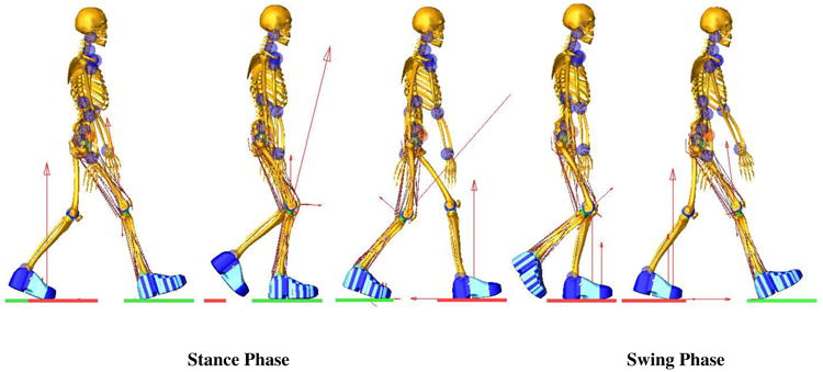
Full body multibody model of the patient with the prosthetic knee during a forward dynamics gait simulation. The red arrows represent the magnitude of joint contact forces and ground reaction forces.
A compliant contact force model was defined between the femoral component and tibial insert geometries to provide computationally efficient characterization of the tibio-femoral contact force. The defined compliant contact force was the ADAMS default IMPACT function that models the contact by a nonlinear equation [20]:
| (1) |
| (2) |
where F is the contact force, δ is the interpenetration of the geometries, kc is a contact stiffness, expc is the exponent, δ˙ is the first derivative of the interpenetration and Bc(δ) is a damping term. The damping Bc(δ) is a function of the interpenetration depths, transition depth dmax and the damping coefficient Bmax.
Guess et al. [21] properties and Hertzian contact theory, as follows: kc = 30,000 N/mm1.5, expc = 1.5, dmax = 0.1 mm and Bmax = 40 Ns/mm. In the context of rigid body system dynamics, where Hertzian contact theory relates the contact force to resultant penetration [22], using Hertzian contact theory provides a suitable solution for articulations between the plastic and metal components.
The IMPACT function also includes a built-in Coulomb friction equation that defines contact coefficients as a function of slip velocity [20]:
| (3) |
Where v is the slip velocity at the contact point, μs is the static coefficient, μd is the dynamic coefficient, vs is the stiction transition velocity and vd is the friction transition velocity. The static coefficient, dynamic coefficient, stiction transition velocity, and friction transition velocity were assumed to be 0.15, 0.07, 100, and 1000 mm/sec respectively [23].
The detailed right knee model was constrained by contact between the knee component geometries and ligament forces. The model included three bundles for the lateral collateral ligaments (LCL), three bundles for the medial collateral ligaments (MCL), and one bundle for the posterior cruciate ligament (PCL) as the PCL was preserved during implant surgery [1]. Ligament bundles were represented in the model as a single force element with a nonlinear force-strain curve [24]:
| (4) |
| (5) |
Where k is a stiffness parameter and ε is defined as the engineering strain. The spring parameter εl is a constant value and it was assumed to be 0.03 [24]. The ligament stiffness parameter k was 2000 N for all the bundles of the LCL, 2750 N for the bundles of the MCL, and 9000 N for the single bundle of the PCL [24]. The zero-load lengths l0 and ligament insertions and origins were estimated based on previous cadaveric studies performed by Guess et al [25-27]. Each force element also included a parallel damper coefficient with a small value of 0.5 NS/mm to remove the possibility of high frequency vibrations during simulation [26]. The patellar tendon was divided into three bundles which were modeled as tension only linear springs with a stiffness of 580 N/mm. This numerical value was adjusted by studying the position of the patella in the femoral groove during forward dynamics simulations.
Shoe–floor interaction was modeled with deformable contacts (Eqs. 1 and 2) between shoe geometries and the floor. The Coulomb friction was included in the contact with a static friction coefficient of 1.0 and a dynamic friction coefficient of 0.8 [28]. To allow for different contact parameters to be used depending on shoe location and to allow for future comparisons with measured foot ground contact pressures, a macro was written in ADAMS to automatically divide the right shoe geometry into 90 pieces. The left shoe was only divided into heel, mid-foot, and toe regions. Due to contact geometries at heel strike, the contact parameters for the heel region were lower than the mid-foot and toe regions (Table. 1). A hinge joint was applied where the mid-foot region joins the toe region to model the metatarsophalangeal joints. Shoe geometries were attached rigidly to either the sole or ball of the foot.
Table 1.
Shoe-floor contact parameters defined in heel, mid-foot, and toe regions under the sole and ball of the foot.
| Stiffness (N/mm) | Damping (N.sec/mm) | Exponent | |
|---|---|---|---|
| Heel | 20.0 | 0.20 | 1.00 |
| Mid-Foot | 200 | 2.00 | 1.00 |
| Toe | 200 | 2.00 | 1.00 |
LifeMOD was used to place forty-five muscles onto the right lower extremity. LifeMOD is a virtual human modeling and simulation software add-on to ADAMS and contains a data base of muscle properties including the muscle insertion origin and model muscle wrapping via points. The attachments of the quadriceps muscles were modified to insert on the patella and the hamstring and gastrocnemius insertions were modified based on developed knee geometries from CT data.
The measured kinematics, collected during two trials each of normal, medial thrust, and trunk sway gaits, were used to drive the inverse kinematics simulation. The muscle-tendon shortening/lengthening patterns as well as joint motions of the upper body and left leg were recorded in the inverse kinematics step. Next the kinematic constraints were removed and muscles and joints served as actuators to replicate the motions during forward dynamics (Fig. 1). A proportional–integral-derivative (PID) feedback controller was implemented to calculate each muscle force magnitude using the error signal between the current muscle length in the forward dynamics and the recorded muscle length during the inverse kinematics simulation. The PID controllers replicate the desired motion by minimizing the error signals, Eqs 5 and 6 [20].
| (5) |
| (6) |
Where Fi is the resulting force for each individual muscle i, lir is the recorded muscle length, lic is the current muscle length, and ROM is the muscle range of motion Ierror. and Derror are defined as the integral and the first derivative of perror with respect to time. In order to account for muscle size, the controller gains (Eq. 5) were multiplied by a scale factor εr defined as the ratio of muscle physiological cross sectional area PCSAi to a reference PCSAr (1500 mm2). Therefore, muscles with greater PCSA had higher gains than muscles with smaller PCSAs.
The force generated by individual muscle was limited by its maximum force generating potential given by the following equation [20]:
| (7) |
Where Fi−max is the muscle maximum force, PCSAi is the default muscle physiological cross sectional area in LifeMOD and σmax is the maximum tissue stress. The σmax was assumed to be 1.7 N/mm2 for all muscles [29, 30]. To maintain a proper balance during the forward dynamics simulation a tracking agent was installed in LifeMOD. The tracking agent is a 6-axis spring located between a “dummy” rigid body and the pelvis. The “dummy” rigid body is driven by kinematic constraints that follow pelvis motion measured during the inverse kinematics simulation. If the forward dynamics motion follows the inverse kinematics motion, the tracking agent will have minimal influence on the model. The tracking agent imparts no force in the vertical direction, regardless of the motion. The average tracking agent forces in the anterior-posterior and medial-lateral directions were less than 38N during all trials. The upper body and lower left extremity joint kinematics were predicted during the forward dynamic simulation through a series of proportional-derivative controllers located at each individual joint. The controller produced the required moments to replicate the recorded joint kinematics from the inverse kinematics step. However, toe kinematics were derived from experimentally measured data.
Evaluation of the model was accomplished by comparing the predicted tibio-femoral contact loads to the measured e-Tibia data (Fig. 2) as well as comparing the predicted and measured ground reaction forces during six gait trials: normal gait (ngait12 and ngait13), trunk sway gait (tsgait1 and tsgait2), and medial thrust gait (mtgait4, and mtgait5). In addition, normalized predicted muscle forces were compared to normalized experimental EMG and predicted ligament forces and patello-femoral contact forces were recorded. The experimental joint contact forces were low-pass filtered with a cut-off frequency of 6 Hz to reduce measurement noise [31]. The contact forces predicted by the model were also passed through a 4th order Butterworth filter with a 6 Hz cut-off frequency. Similarly, the model predicted ground reaction forces and ligament and patella contact forces were low-pass filtered at 6 Hz.
Figure 2.
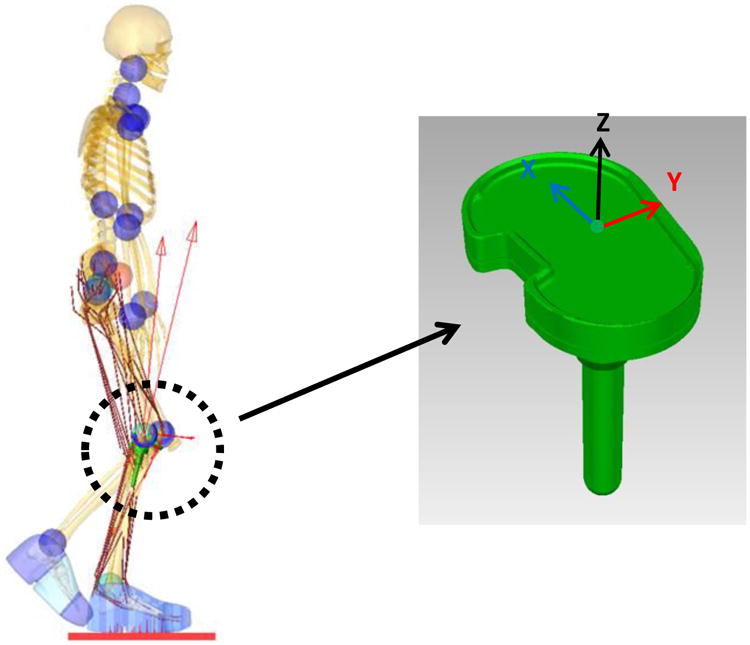
Implemented tibia tray with the e-Tibia coordinate system. X, Y, and Z axes correspond to the lateral–medial (LM), anterior-posterior (AP), and superior-inferior (SI) directions respectively.
The raw EMG measurements from 14 lower extremity muscles on the right leg were collected during each gait trial. Also, a series of maximum voluntary contraction (MVC) efforts were performed by the subject for seven isolated right leg muscle groups and the EMG signals were collected. The provided experimental EMG signals were processed with a high-pass filter with a 30 Hz cut-off frequency, demeaned, rectified, and then low-pass filtered at 6 Hz to eliminate measurement noise [1, 31]. Further, the filtered EMG signals were normalized by dividing by the maximum EMG voltage for each individual muscle from either the MVC or gait trials., The predicted muscle forces during the forward dynamics simulations were normalized to the maximum muscle forces (Fi−max). The experimental and predicted results over the six different trials were compared using mean average deviation MDA, root mean square deviation RMSD and normalized root mean square deviation NRMSD:
| (8) |
| (9) |
| (10) |
Where mi and di indicate the model and experimental value at each time step i, K is the total number of steps △ and is the range of experimental values defined as the difference between the maximum and the minimum value in a data set. Graphical comparisons of predicted data versus the experimental data were provided by normalizing each cycle from 0% to 100% of the gait cycle for all six trials. Predicted force and torque components were averaged across trials and the standard deviation calculated. The normalized EMG profiles and normalized muscle force patterns were also compared between model and experiment by computing the ±1 standard deviation among all gait trials.
Results
Figure 3 provides the model predicted and measured tibia loading for the six gait trials. Computed lateral and medial axial contact force were also compared to the experimental measurements (Fig. 4). Figure 5 and 6 show the model predicted and experimental ground reaction forces, center of pressure (cop), and free vertical moment for the trials respectively. The average model predictions over the six gait trials are shown with a solid line that includes ±1 standard deviation error bars. Experimental measurements are shown with a shaded area corresponding to ±1 standard deviation. Although model predictions of the total axial force acting on the tibial tray had good agreement with the experimental measurements, the model had lower accuracy predicting load distributions on the lateral and medial sides of the tibia (Fig. 3, 4). The gait trial with the lowest e-Tibia tray axial force (Fz) MAD and RMSD was from normal gait trial ngait12. The calculated e-Tibia errors for the MAD and RMSD were 166 N and 212 N respectively with the corresponded MAD and RMSD. The tsgait1trial had the minimum one cycle MAD and RMSD for the vertical ground reaction forces. The calculated vertical ground reaction166 N and 212 N forces for tsgait1 were 67 N and 97.6 N respectively which correspond to an accuracy within 13% of the experimental loads.
Figure 3.
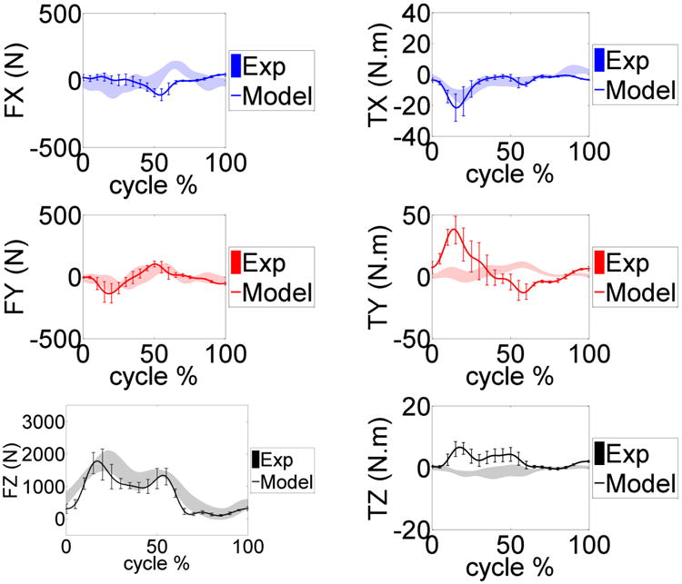
Model predicted and measured e-Tibia forces and torques during the gait trials. The mean and ±1 standard deviation for the six trials is shown.
Figure 4.
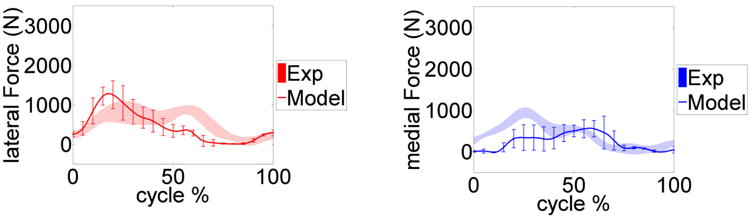
Model predicted and measured e-Tibia forces upon on lateral and medial tibia tray. The mean and ±1 standard deviation for the six trials is shown
Figure 5.
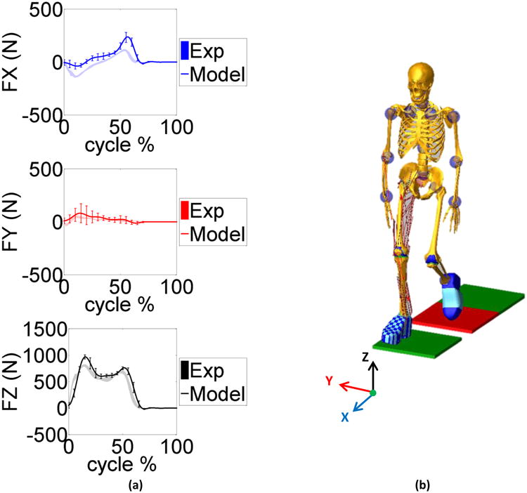
a) Model predicted and measured ground reaction force components in the anterior posterior (FX), medial lateral (FY) and vertical (FZ) directions during the gait trials. The mean and ±1 standard deviation for the six trials is shown. b) A screen shot of model simulation showing walking on the force plates. The X, Y, and Z axes correspond to the anterior-posterior (AP), medial-lateral (ML), and inferior-superior (IS) directions respectively.
Figure 6.
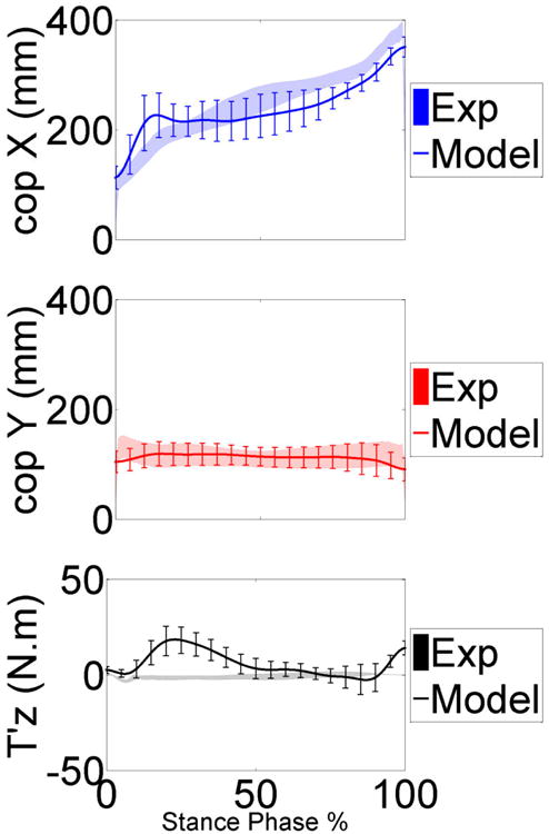
Model predicted and measured center of pressure and free vertical moment in the anterior posterior (cop X), medial lateral (cop Y) and vertical (T'z) directions during the stance phase of gait trials. The mean and ±1 standard deviation for the six trials is shown
Tables 2-4 summarize the MAD, RMSD, and NRMSD for the e-Tibia forces, torques and foot-ground reaction forces as well as the predicted joint kinematics for all six gait trials. The kinematics results are presented in terms of flexion-extension (FE), internal-external (IE), and adduction-abduction (AA) rotations. The muscle driven forward dynamics models were able to accurately reproduce the kinematics of the hip and ankle joint (RMSD < 2.70). The normalized averaged EMG patterns for the medial gastrocnemius, soleus, vastus medialis, vastus lateralis, biceps femoris and the tibialis anterior were plotted in Figure 7. The predicted pattern and timing of muscle forces was compared with the measured EMG signals. The patello-femoral contact force was recorded during simulation (Fig.8). The maximum patello-femoral contact force occurred in the early mid stance phase (Fig. 8). Figure 9 shows the calculated average ligament forces for all six gait cycles within the ±1 standard deviation. The net force in the respective ligaments was the result of adding up the force magnitude of all individual bundles. The peak ligament force was 200 N in the late swing phase and was similar in all six trials. Animations of forward dynamics simulations for the three gait types as well as additional figures are provided as supplemental files.
Table 2.
Calculated mean absolute deviation (MAD), root mean square deviation (RMSD) and normalized RMSD for simulation results during the normal gaits.
| Normal Gait (ngait #) | |||||||
|---|---|---|---|---|---|---|---|
| ngait 12 | ngait 13 | ||||||
| MAD | RMSD | NRMSD | MAD | RMSD | NRMSD | ||
| (N) | (N) | (%) | (N) | (N) | (%) | ||
| e-Tibia Forces | Fx (LM) | 80.7 | 90.7 | 47.0 | 67.3 | 77.8 | 45.6 |
| Fy (AP) | 41.8 | 51.9 | 26.6 | 39.9 | 46.4 | 33.0 | |
| Fz (SI) | 166 | 212 | 14.8 | 271 | 335 | 18.7 | |
| Fz (lateral) | 276 | 324 | 41.9 | 325 | 399 | 40.9 | |
| Fz (medial) | 372 | 434 | 49.8 | 208 | 263 | 24.4 | |
| MAD | RMSD | NRMSD | MAD | RMSD | NRMSD | ||
| (N.m) | (N.m) | (%) | (N.m) | (N.m) | (%) | ||
| e-Tibia Torques | Tx | 1.98 | 2.47 | 20.2 | 3.57 | 4.43 | 24.7 |
| Ty | 14.3 | 17.4 | 120 | 8.83 | 11.1 | 102 | |
| Tz | 2.01 | 2.44 | 111 | 2.14 | 2.88 | 114 | |
| MAD | RMSD | NRMSD | MAD | RMSD | NRMSD | ||
| (N) | (N) | (%) | (N) | (N) | (%) | ||
| GRF | Fx (AP) | 50.2 | 71.3 | 28.9 | 54.3 | 79.0 | 30.5 |
| Fy (ML) | 25.7 | 34.9 | 51.0 | 20.0 | 29.1 | 36.5 | |
| Fz (IS) | 66.8 | 111 | 14.1 | 76.3 | 126 | 15.5 | |
| cop (X) | 35.3 | 47.8 | 14.3 | 15.6 | 27.8 | 8.40 | |
| cop (Y) | 8.20 | 12.7 | 13.2 | 11.9 | 15.4 | 14.3 | |
| T'z | 5.50 | 6.10 | 127 | 5.40 | 7.30 | 212 | |
| MAD | RMSD | NRMSD | MAD | RMSD | NRMSD | ||
| (deg) | (deg) | (%) | (deg) | (deg) | (%) | ||
| Kinematics | Hip FE | 1.20 | 1.40 | 3.40 | 1.00 | 1.20 | 2.70 |
| Hip IE | 0.80 | 1.00 | 8.90 | 0.60 | 0.70 | 10.5 | |
| Hip AA | 0.60 | 0.70 | 3.20 | 0.60 | 0.70 | 3.80 | |
| Ankle FE | 1.30 | 1.60 | 4.50 | 1.30 | 1.40 | 4.30 | |
| Ankle IE | 1.30 | 1.80 | 14.3 | 1.3 | 1.70 | 17.7 | |
| Ankle AA | 1.30 | 1.40 | 12.5 | 1.5 | 1.70 | 13.0 | |
Table 4.
Calculated mean absolute deviation (MAD), root mean square deviation (RMSD) and normalized RMSD for simulation results during the medial thrust gaits.
| Medial Thrust Gait (mtgait #) | |||||||
|---|---|---|---|---|---|---|---|
| mtgait 4 | mtgait 5 | ||||||
| MAD | RMSD | NRMSD | MAD | RMSD | NRMSD | ||
| (N) | (N) | (%) | (N) | (N) | (%) | ||
| e-Tibia Forces | Fx (LM) | 74.0 | 89.2 | 39.7 | 106.4 | 122 | 43.0 |
| Fy (AP) | 74.3 | 94.5 | 47.0 | 50.1 | 70.1 | 38.7 | |
| Fz (SI) | 405 | 447 | 27.4 | 376 | 413 | 21.7 | |
| Fz (lateral) | 310 | 376 | 39.6 | 456 | 548 | 56.7 | |
| Fz (medial) | 289 | 357 | 44.3 | 247 | 294 | 29.7 | |
| MAD | RMSD | NRMSD | MAD | RMSD | NRMSD | ||
| (N.m) | (N.m) | (%) | (N.m) | (N.m) | (%) | ||
| e-Tibia Torques | Tx | 2.66 | 3.46 | 14.6 | 6.27 | 8.41 | 32.8 |
| Ty | 13.0 | 17.6 | 130 | 14.71 | 18.26 | 143 | |
| Tz | 4.45 | 5.99 | 136 | 3.10 | 4.00 | 94.0 | |
| MAD | RMSD | NRMSD | MAD | RMSD | NRMSD | ||
| (N) | (N) | (%) | (N) | (N) | (%) | ||
| GRF | Fx (AP) | 53.9 | 67.5 | 26.1 | 40.8 | 59.3 | 23.8 |
| Fy (ML) | 27.5 | 39.9 | 41.2 | 19.6 | 28.0 | 30.0 | |
| Fz (IS) | 89.1 | 127.4 | 15.7 | 76.0 | 110 | 13.2 | |
| cop (X) | 40.8 | 46.3 | 14.0 | 31.7 | 40.9 | 11.1 | |
| cop (Y) | 7.30 | 11.1 | 13.6 | 10.5 | 14.6 | 11.7 | |
| T'z | 8.30 | 10.6 | 167 | 8.8 | 11.4 | 177 | |
| MAD | RMSD | NRMSD | MAD | RMSD | NRMSD | ||
| (deg) | (deg) | (%) | (deg) | (deg) | (%) | ||
| Kinematics | Hip FE | 1.80 | 2.00 | 5.00 | 1.70 | 1.90 | 5.00 |
| Hip IE | 0.90 | 1.00 | 6.10 | 0.90 | 1.00 | 7.00 | |
| Hip AA | 0.80 | 0.90 | 5.90 | 0.90 | 1.00 | 6.00 | |
| Ankle FE | 1.70 | 2.10 | 7.90 | 1.90 | 2.30 | 9.00 | |
| Ankle IE | 1.90 | 2.50 | 13.4 | 1.80 | 2.60 | 26.1 | |
| Ankle AA | 1.60 | 1.90 | 13.0 | 1.50 | 1.70 | 12.0 | |
Figure 7.
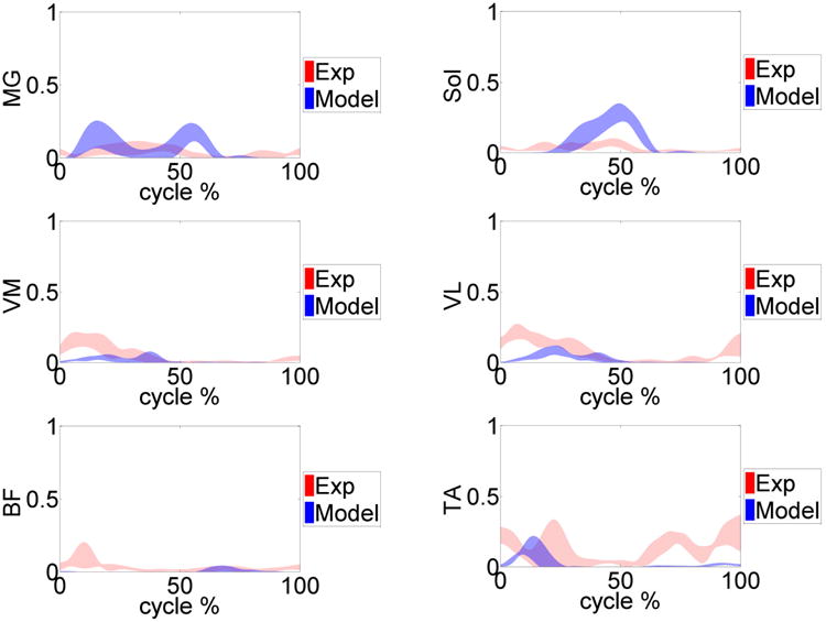
Measured normalized EMG (red) versus model predicted muscle forces (blue) for the primary muscles involved during the gait trials. Medial gastrocnemius (MG), soleus (Sol), vastus medialis (VM), vastus lateralis (VL), biceps femoris (BF) and the tibialis anterior (TA) muscles are shown.
Figure 8.
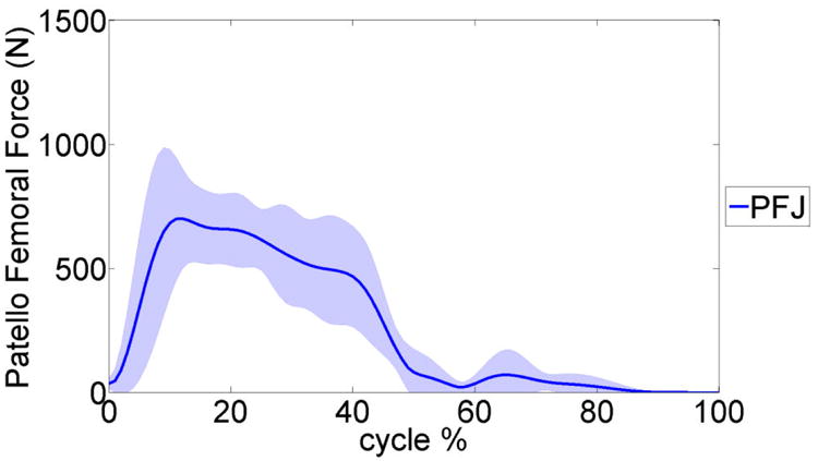
The average predicted patello-femoral joint (PFJ) contact force during the six gait trials. The shaded area presents a ±1 standard deviation.
Figure 9.
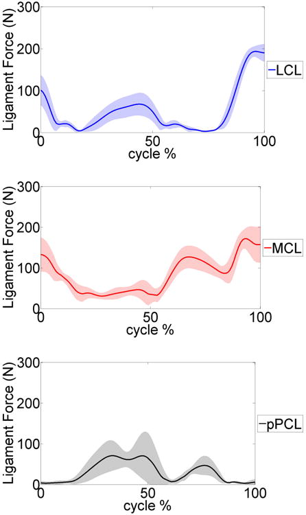
Average predicted lateral collateral ligament (LCL), medial collateral ligament (MCL) and posterior cruciate ligament (pPCL) forces during the six gait trials. The shaded area represents a ±1 standard deviation.
Discussion
This study produced a subject specific musculoskeletal model capable of concurrent simulation of joint contact mechanics, foot-ground interactions, and muscle and ligament forces. The 2011 Grand Challenge Data sets provide a unique opportunity to evaluate the method by comparing the predicted results with the measured experimental data. An instrumented knee prosthesis that continuously measured all six load components on the tibia tray was used to measure the knee loads during the experiments (e-Tibia loads) [1]. Model predicted e-Tibia force and torque patterns have overall agreement in comparison to the experimental measurements (Fig. 3) during six gait trials. However some discrepancy was observed between the measured e-Tibia loads and the model predictions, particularly in the lateral-medial force (Fx), the abduction-adduction moment (Ty) and the superior-inferior moment (Tz). The minimum mean absolute deviation (MAD) and root mean square deviation (RMSD) of the e-Tibia axial load (Fz) occurred in normal gait ngait12 with values of 166 N and 212 N respectively. These values correspond to accuracy within 15% of the experimental loads (Table. 2). The maximum prediction MAD and RMSD load occurred during medial thrust gait mtgait4 and were 404 and 447 N respectively. These values correspond to accuracy within 28% of the experimental loads (Table 4).
The highest deviation was in the adduction-abduction moment (Ty) for all models (Tables. 2-4). The high deviation in the adduction-abduction moment can be attributed to incorrect muscle force predictions, inaccuracies in muscle moment arms, ground reaction forces and center of pressure location. Even though the ground reaction forces are predicted accurately there is a high deviation in the vertical ground reaction moment (Fig. 6) especially in the first half of the stance phase of gait. The center of pressure location is predicted accurately (Fig. 6) but any small deviations can affect adduction-abduction moment in the knee joint because of the long moment arm (length of lower leg segment). The predicted muscle forces can only be evaluated against a limited number of muscles sampled with EMG during the experiment and any comparisons are purely in regards to timing of the activation. Correct prediction of muscle forces is extremely important in resolving the medial-lateral distribution of knee contact loads. Several studies using computational models have predicted total contact forces within ranges of the experimentally measured forces but none were able to resolve the medial-lateral distributions accurately [1]. In our model the muscle forces are predicted using a PID control scheme which has some limitations since the controller is only matching the muscle length patterns. In addition, applying a conventional PID controller scheme may be inadequate to model the highly nonlinear and dynamic neuromusculoskeletal system [32].
The predicted ground reaction forces followed the experimentally measured force very well in all directions (Fig.4). During the early stance (10 to 20%) the predicted vertical load (Fz) and the medial-lateral force (Fy) had their highest deviation. The predicted anterior-posterior force (Fx) was underestimated for most of the cycle except at late stance (50 to 60%). These highlighted points relate to the time where the contralateral limb was close to push off and toe-off. In the current study the contralateral limb was modeled by mirroring the right side and assuming a simplified joint for the knee joint. In addition, the toe regions of the shoes were rigid and did not allow for shoe compliance and bending during toe-off.
A feedback control approach was applied to calculate each muscle force magnitude and their activation times by reducing the calculated error signal between the current muscle length in the forward dynamics and the recorded muscle length during the inverse kinematics simulation. During the initial loading response (heel strike), all the primary muscles are activated to oppose the hip flexion and provide stability at the knee joint. Directly after contralateral toe-off the vastus medialis and vastus lateralis (quadriceps muscle group) acted to extend the knee, activating these muscles during mid-stance. In contrast, the gastrocnemius and soleus acted during the late-stance to flex the knee while creating an ankle plantar-flexion. Although the feedback control method was efficient and fast and could replicate the motions very well, this method could not adequately predict the co-contraction of antagonistic muscles such as the biceps femoris and the tibialis anterior during gait (Fig. 5). The estimated force by the PID feedback control scheme depends on muscle shortening-lengthening curves over time, while real muscles can produce force without a change in the length, in which case the PID controllers may not estimate the force accurately. Therefore applying more sophisticated muscle model strategies to predict muscle forces and adapting muscle attachment sites based on subject specific MRI is recommended. The muscle prediction algorithm can be improved by incorporating the experimental EMG traces when available and by using Hill models for some of the muscles that are active without significant changes in length. This technique can be applied along with the PID control scheme to compensate for the conventional feedback control weaknesses as well as enhance the predictions on muscle force dynamics. Moreover, an optimization cost function such as minimizing muscle stress can be imposed on the force predictions to generate more realistic muscle force patterns [33].
The error in hip and ankle joint motions determined during forward dynamics was compared to the inverse kinematics. Results indicated that the muscle driven forward dynamic solutions accurately replicate motion of the inverse kinematic simulations. Guess et al. [21] applied the IMPACT function in ADAMS, which models the contact as a nonlinear power function of penetration depth and velocity. Hertzian contact theory was then utilized to estimate contact parameters based on material properties and approximating the articular surface curvatures with fitted ellipsoids. The effect of several scaled ellipsoid dimension to predicted ankle kinematics were examined. Their result indicated that modifying the ellipsoid's size could change ankle vertical rotation but had no significant effect on other directions [21]. In the present study, the same contact parameters were considered. However, sensitivity analysis can be performed in the future to evaluate joint kinematics as well as kinetics for different implanted knee geometries.
The model was also able to calculate and predict the patello-femoral contact and ligament forces simultaneously during the gait cycle (Fig. 6, 7). The model simulation predicted that the patello-femoral joint was loaded during the stance phase of gait and it was unloaded during the swing phase. The patello-femoral peak force ranged from 809 N to 1200 N (∼ 1.2 to 1.8 BW) (Table. 5). The computed patello-femoral force, predicted in our models, was in the same range as that reported by Ward and Powers [34]. In their study with a simpler model, the patello-femoral contact forces ranged between 400 – 800N. Similarly in a study by Shelburne et al. the patello-femoral peak force during gait was approximately 250N and the time pattern of loading was very similar to our predictions [35]. In a study by Lin et al [36] the peak patello-femoral contact force was approximately 250N which is significantly smaller. The magnitude of the ligament forces calculated in the current study is depicted in Figure 7. The material properties of the ligaments were taken from previous studies [25-27]. The largest forces occurred in the MCL and LCL and they both were approximately 200 N at the end of swing phase. The maximum force of 150 N occurred in the PCL, approximately at mid-stance, to provide resistance to the tibia rotation. These results were comparable with other published studies [35, 37]. For example in a computational study by Shelburne et al. [35] the peak collateral ligament forces were 167N. Between ground reaction forces, muscle forces and ligament forces the smallest contribution to tibio-femoral contact force during gait is by the ligaments [38], therefore our ligament force predictions are unlikely to be contributing to any errors in the contact force predictions. Morrison et al. [37] noted that the forces in knee ligaments can vary significantly between individuals due to subject specific gait characteristics and knee joint geometries. This would suggest that using subject specific magnetic resonance images (MRI) along with the knee laxity test to estimate ligament properties will improve the model predictions.
Table 5.
Maximum and mean value of patello-femoraljoint contact force (PFJ) during the gait trials.
| PFJ Contact | Normal gait | Trunk sway gait | Medial thrust gait | |||
|---|---|---|---|---|---|---|
| ngait12 | ngait13 | tsgait1 | tsgait2 | mtgait4 | mtgait5 | |
| Maximum value (N) | 823 | 914 | 809 | 947 | 758 | 1221 |
| Mean value (N) | 225 | 276 | 184 | 305 | 243 | 292 |
In summary this study evaluates the force predictions of a musculoskeletal movement simulation over six different gait simulations. Computational models that combine muscle force predictions with subject specific joint anatomy can be a valuable tool for understanding the relationships of joint loading and motor control. In the current study only the net knee forces and torques were predicted and compared with the experimental knee loads (e-Tibia). In the future the tibia insert will be divided into smaller elements with separate deformable contacts for each individual element. This method was found to be powerful in determining contact pressure distribution within the multibody frame work [27]. We also implemented a muscle force prediction method that uses the muscle length patterns recorded during inverse kinematics in a PID scheme to efficiently generate muscle forces for the muscle driven forward simulation. Although, the feedback control scheme did not accurately predict the motor control patterns, this method can be the starting point for development of an efficient way to generate realistic muscle forces. Overall the model predicted ground reaction and total tibio-femoral contact forces accurately in multiple trials for three different gait patterns.
Supplementary Material
Table 3.
Calculated mean absolute deviation (MAD), root mean square deviation (RMSD) and normalized RMSD for simulation results during the trunk sway gaits.
| Trunk Sway Gait (tsgait #) | |||||||
|---|---|---|---|---|---|---|---|
| tsgait 1 | tsgait 2 | ||||||
| MAD | RMSD | NRMSD | MAD | RMSD | NRMSD | ||
| (N) | (N) | (%) | (N) | (N) | (%) | ||
| e-Tibia Forces | Fx (LM) | 60.2 | 76.8 | 27.0 | 67.3 | 80.4 | 37.2 |
| Fy (AP) | 42.7 | 51.8 | 20.6 | 41.7 | 53.1 | 29.4 | |
| Fz (SI) | 211 | 258 | 14.0 | 178 | 232 | 14.0 | |
| Fz (lateral) | 13.0 | 17.2 | 158 | 13.1 | 17.2 | 157 | |
| Fz (medial) | 4.28 | 5.34 | 103 | 3.01 | 4.12 | 122 | |
| MAD | RMSD | NRMSD | MAD | RMSD | NRMSD | ||
| (N.m) | (N.m) | (%) | (N.m) | (N.m) | (%) | ||
| e-Tibia Torques | Tx | 3.58 | 5.25 | 35.1 | 2.67 | 3.03 | 15.7 |
| Ty | 13.03 | 17.2 | 158 | 13.1 | 17.2 | 157 | |
| Tz | 4.29 | 5.34 | 103 | 3.01 | 4.12 | 122 | |
| MAD | RMSD | NRMSD | MAD | RMSD | NRMSD | ||
| (N) | (N) | (%) | (N) | (N) | (%) | ||
| GRF | Fx (AP) | 47.6 | 65.1 | 23.8 | 44.0 | 62.1 | 25.0 |
| Fy (ML) | 23.2 | 30.3 | 32 | 31.3 | 42.5 | 50.0 | |
| Fz (IS) | 72.2 | 106 | 13.2 | 67.1 | 97.6 | 12.3 | |
| cop (X) | 31.8 | 37.6 | 10.7 | 37.0 | 41.7 | 13.2 | |
| cop (Y) | 6.40 | 10.4 | 12.9 | 7.40 | 10.3 | 12.0 | |
| T'z | 14.14 | 16.5 | 376 | 8.10 | 10.0 | 264 | |
| MAD | RMSD | NRMSD | MAD | RMSD | NRMSD | ||
| (deg) | (deg) | (%) | (deg) | (deg) | (%) | ||
| Kinematics | Hip FE | 1.40 | 1.40 | 3.00 | 1.30 | 1.30 | 3.10 |
| Hip IE | 0.80 | 0.80 | 5.70 | 1.00 | 1.00 | 6.90 | |
| Hip AA | 0.80 | 0.80 | 4.90 | 0.70 | 0.70 | 3.50 | |
| Ankle FE | 1.50 | 2.00 | 6.30 | 1.60 | 2.00 | 6.50 | |
| Ankle IE | 1.70 | 2.40 | 21.5 | 1.40 | 2.20 | 15.3 | |
| Ankle AA | 1.50 | 1.80 | 19.0 | 1.50 | 1.60 | 15.8 | |
Acknowledgments
The authors would like to thank Dr. B.J. Fregly and colleagues for providing the publicly accessible data.
Funding: Portions of this research were funded by the Missouri Life Sciences Research Board, Award Number 09-1078 and by the National Institute of Arthritis and Musculoskeletal and Skin Diseases, Award NumberR15AR061698.
Footnotes
Competing interests: None declared
Ethical approval: Not required
Contributor Information
Mohammad Kia, Email: kiam@hss.edu, Department of Biomechanics, Hospital for Special Surgery, 535 East 70 th St. New York, NY10021, Tel.:(212) 774-7275.
Antonis P. Stylianou, Email: stylianoua@umkc.edu, Musculoskeletal Biomechanics Research Laboratory, Department of Civil and Mechanical Engineering, University of Missouri – Kansas City, 5100 Rockhill Road, Kansas City, MO 64110-2499, Tel.: (816) 235-6390.
Trent M. Guess, Email: guesstr@missouri.edu, Departments of Physical Therapy and Orthopaedic Surgery, University of Missouri, 801 Clark Hall, Columbia, MO 65211-4250, Tel.: (573) 882-1734.
References
- 1.Fregly BJ, Besier TF, Lloyd DG, Delp SL, Banks SA, Pandy MG, D'Lima DD. Grand challenge competition to predict in vivo knee loads. J Orthop Res. 2012;30(4):503–13. doi: 10.1002/jor.22023. [DOI] [PMC free article] [PubMed] [Google Scholar]
- 2.Huang A, Hull ML, Howell SM. The level of compressive load affects conclusions from statistical analyses to determine whether a lateral meniscal autograft restores tibial contact pressure to normal: a study in human cadaveric knees. J Orthop Res. 2003;21(3):459–64. doi: 10.1016/S0736-0266(02)00201-2. [DOI] [PubMed] [Google Scholar]
- 3.Kuroda R, Kambic H, Valdevit A, Andrish JT. Articular cartilage contact pressure after tibial tuberosity transfer. A cadaveric study. Am J Sports Med. 2001;29(4):403–9. doi: 10.1177/03635465010290040301. [DOI] [PubMed] [Google Scholar]
- 4.Ronsky JL, Herzog W, Brown TD, Pedersen DR, Grood ES, Butler DL. In vivo quantification of the cat patellofemoral joint contact stresses and areas. J Biomech. 1995;28(8):977–83. doi: 10.1016/0021-9290(94)00153-u. [DOI] [PubMed] [Google Scholar]
- 5.Heinlein B, Kutzner I, Graichen F, Bender A, Rohlmann A, Halder AM, Beier A, Bergmann G. ESB Clinical Biomechanics Award 2008: Complete data of total knee replacement loading for level walking and stair climbing measured in vivo with a follow-up of 6-10 months. Clin Biomech (Bristol, Avon) 2009;24(4):315–26. doi: 10.1016/j.clinbiomech.2009.01.011. [DOI] [PubMed] [Google Scholar]
- 6.Kutzner I, Heinlein B, Graichen F, Bender A, Rohlmann A, Halder A, Beier A, Bergmann G. Loading of the knee joint during activities of daily living measured in vivo in five subjects. J Biomech. 2010;43(11):2164–73. doi: 10.1016/j.jbiomech.2010.03.046. [DOI] [PubMed] [Google Scholar]
- 7.Barink M, van Kampen A, de Waal Malefijt M, Verdonschot N. A three-dimensional dynamic finite element model of the prosthetic knee joint: simulation of joint laxity and kinematics. Proc Inst Mech Eng H. 2005;219(6):415–24. doi: 10.1243/095441105X34437. [DOI] [PubMed] [Google Scholar]
- 8.Donahue TL, Hull ML, Rashid MM, Jacobs CR. A finite element model of the human knee joint for the study of tibio-femoral contact. J Biomech Eng. 2002;124(3):273–80. doi: 10.1115/1.1470171. [DOI] [PubMed] [Google Scholar]
- 9.Halloran JP, Clary CW, Maletsky LP, Taylor M, Petrella AJ, Rullkoetter PJ. Verification of predicted knee replacement kinematics during simulated gait in the Kansas knee simulator. J Biomech Eng. 2010;132(8):081010. doi: 10.1115/1.4001678. [DOI] [PubMed] [Google Scholar]
- 10.Halloran JP, Easley SK, Petrella AJ, Rullkoetter PJ. Comparison of deformable and elastic foundation finite element simulations for predicting knee replacement mechanics. J Biomech Eng. 2005;127(5):813–8. doi: 10.1115/1.1992522. [DOI] [PubMed] [Google Scholar]
- 11.Halloran JP, Petrella AJ, Rullkoetter PJ. Explicit finite element modeling of total knee replacement mechanics. J Biomech. 2005;38(2):323–31. doi: 10.1016/j.jbiomech.2004.02.046. [DOI] [PubMed] [Google Scholar]
- 12.Zielinska B, Donahue TL. 3D finite element model of meniscectomy: changes in joint contact behavior. J Biomech Eng. 2006;128(1):115–23. doi: 10.1115/1.2132370. [DOI] [PubMed] [Google Scholar]
- 13.Adouni M, Shirazi-Adl A, Shirazi R. Computational biodynamics of human knee joint in gait: from muscle forces to cartilage stresses. J Biomech. 2012;45(12):2149–56. doi: 10.1016/j.jbiomech.2012.05.040. [DOI] [PubMed] [Google Scholar]
- 14.Beillas P, Lee SW, Tashman S, Yang KH. Sensitivity of the tibio-femoral response to finite element modeling parameters. Comput Methods Biomech Biomed Engin. 2007;10(3):209–21. doi: 10.1080/10255840701283988. [DOI] [PubMed] [Google Scholar]
- 15.Chang CY, Rupp JD, Reed MP, Hughes RE, Schneider LW. Predicting the effects of muscle activation on knee, thigh, and hip injuries in frontal crashes using a finite-element model with muscle forces from subject testing and musculoskeletal modeling. Stapp Car Crash J. 2009;53:291–328. doi: 10.4271/2009-22-0011. [DOI] [PubMed] [Google Scholar]
- 16.Mesfar W, ShiraziAdl A. Knee joint biomechanics in open-kinetic-chain flexion exercises. Clin Biomech (Bristol, Avon) 2008;23(4):477–82. doi: 10.1016/j.clinbiomech.2007.11.016. [DOI] [PubMed] [Google Scholar]
- 17.Zelle J, Heesterbeek PJ, De Waal Malefijt M, Verdonschot N. Numerical analysis of variations in posterior cruciate ligament properties and balancing techniques on total knee arthroplasty loading. Med Eng Phys. 2010;32(7):700–7. doi: 10.1016/j.medengphy.2010.04.013. [DOI] [PubMed] [Google Scholar]
- 18.Spagele T, Kistner A, Gollhofer A. Modelling, simulation and optimisation of a human vertical jump. J Biomech. 1999;32(5):521–30. doi: 10.1016/s0021-9290(98)00145-6. [DOI] [PubMed] [Google Scholar]
- 19.Piazza SJ, Delp SL. Three-dimensional dynamic simulation of total knee replacement motion during a step-up task. J Biomech Eng. 2001;123(6):599–606. doi: 10.1115/1.1406950. [DOI] [PubMed] [Google Scholar]
- 20.Lifemodeler I. Lifemod Manual. 2010 [Google Scholar]
- 21.Guess TM, Maletsky LP. Computational modelling of a total knee prosthetic loaded in a dynamic knee simulator. Med Eng Phys. 2005;27(5):357–67. doi: 10.1016/j.medengphy.2004.11.003. [DOI] [PubMed] [Google Scholar]
- 22.Adams GG, Nosonovsky M. Contact modeling — forces. Tribology International. 2000;33:431–442. [Google Scholar]
- 23.Sathasivam S, Walker PS. A computer model with surface friction for the prediction of total knee kinematics. J Biomech. 1997;30(2):177–84. doi: 10.1016/s0021-9290(96)00114-5. [DOI] [PubMed] [Google Scholar]
- 24.Blankevoort L, Kuiper JH, Huiskes R, Grootenboer HJ. Articular contact in a three-dimensional model of the knee. J Biomech. 1991;24(11):1019–31. doi: 10.1016/0021-9290(91)90019-j. [DOI] [PubMed] [Google Scholar]
- 25.Guess TM, Liu H, Bhashyam S, Thiagarajan G. A multibody knee model with discrete cartilage prediction of tibio-femoral contact mechanics. Comput Methods Biomech Biomed Engin. 2011 doi: 10.1080/10255842.2011.617004. [DOI] [PubMed] [Google Scholar]
- 26.Guess TM, Thiagarajan G, Kia M, Mishra M. A subject specific multibody model of the knee with menisci. Med Eng Phys. 2010;32(5):505–15. doi: 10.1016/j.medengphy.2010.02.020. [DOI] [PubMed] [Google Scholar]
- 27.Guess TM, Stylianou A. Simulation of anterior cruciate ligament deficiency in a musculoskeletal model with anatomical knees. Open Biomed Eng J. 2012;6:23–32. doi: 10.2174/1874230001206010023. [DOI] [PMC free article] [PubMed] [Google Scholar]
- 28.Nigg BM, Macintosh BR, Mester J. Biomechanics and Biology of Movement. 2000 [Google Scholar]
- 29.Li L, Tong K, Song R, Koo TK. Is maximum isometric muscle stress the same among prime elbow flexors? Clin Biomech (Bristol, Avon) 2007;22(8):874–83. doi: 10.1016/j.clinbiomech.2007.06.001. [DOI] [PubMed] [Google Scholar]
- 30.McMahon TA. Muscles, Reflexes, and Locomotion. Princeton, NJ: Princeton University Press; 1984. [Google Scholar]
- 31.Meyer AJ, D'Lima DD, Besier TF, Lloyd DG, Colwell CW, Jr, Fregly BJ. Are external knee load and EMG measures accurate indicators of internal knee contact forces during gait? J Orthop Res. 2013;31(6):921–9. doi: 10.1002/jor.22304. [DOI] [PMC free article] [PubMed] [Google Scholar]
- 32.Ghafari AS, Meghdari A, Vossoughi GR. Forward dynamics simulation of human walking employing an iterative feedback tuning approach. Systems and Control Engineering. 2008;223:289–97. [Google Scholar]
- 33.Crowninshield RD, Brand RA. A physiologically based criterion of muscle force prediction in locomotion. J Biomech. 1981;14(11):793–801. doi: 10.1016/0021-9290(81)90035-x. [DOI] [PubMed] [Google Scholar]
- 34.Ward SR, Powers CM. The influence of patella alta on patellofemoral joint stress during normal and fast walking. Clin Biomech (Bristol, Avon) 2004;19(10):1040–7. doi: 10.1016/j.clinbiomech.2004.07.009. [DOI] [PubMed] [Google Scholar]
- 35.Shelburne KB, Torry MR, Pandy MG. Muscle, ligament, and joint-contact forces at the knee during walking. Med Sci Sports Exerc. 2005;37(11):1948–56. doi: 10.1249/01.mss.0000180404.86078.ff. [DOI] [PubMed] [Google Scholar]
- 36.Lin YC, Walter JP, Banks SA, Pandy MG, Fregly BJ. Simultaneous prediction of muscle and contact forces in the knee during gait. J Biomech. 2010;43(5):945–52. doi: 10.1016/j.jbiomech.2009.10.048. [DOI] [PubMed] [Google Scholar]
- 37.Morrison JB. The mechanics of the knee joint in relation to normal walking. J Biomech. 1970;3(1):51–61. doi: 10.1016/0021-9290(70)90050-3. [DOI] [PubMed] [Google Scholar]
- 38.Shelburne KB, Torry MR, Pandy MG. Contributions of muscles, ligaments, and the ground-reaction force to tibiofemoral joint loading during normal gait. J Orthop Res. 2006;24(10):1983–90. doi: 10.1002/jor.20255. [DOI] [PubMed] [Google Scholar]
Associated Data
This section collects any data citations, data availability statements, or supplementary materials included in this article.