Fully automatic and robust 3D registration of serial-section microscopic images

Abstract

Robust and fully automatic 3D registration of serial-section microscopic images is critical for detailed anatomical reconstruction of large biological specimens, such as reconstructions of dense neuronal tissues or 3D histology reconstruction to gain new structural insights. However, robust and fully automatic 3D image registration for biological data is difficult due to complex deformations, unbalanced staining and variations on data appearance. This study presents a fully automatic and robust 3D registration technique for microscopic image reconstruction, and we demonstrate our method on two ssTEM datasets of drosophila brain neural tissues, serial confocal laser scanning microscopic images of a drosophila brain, serial histopathological images of renal cortical tissues and a synthetic test case. The results show that the presented fully automatic method is promising to reassemble continuous volumes and minimize artificial deformations for all data and outperforms four state-of-the-art 3D registration techniques to consistently produce solid 3D reconstructed anatomies with less discontinuities and deformations.

Robust and fully automatic three-dimensional (3D) image registration of serial-section microscopic images is critical for detailed 3D anatomical reconstruction of large biological specimens such as serial section Transmission Electron Microscopy (ssTEM) of neural tissues¹, serial confocal laser scanning microscopic images of a brain²,³ or serial histopathological microscopic images⁴,⁵. In biomedical applications, a large specimen is generally embedded in the medium block and cut into a series of microscopy image slices, called as sections, which are collected, stained and digitally imaged. The digital microscopic slices are then used to reconstruct detailed the 3D anatomy for further biological and medical investigation. Serial slides can be manually aligned by setting up a number of pairs of corresponding control points to the same (x, y) location for consecutive images z_i and z_i+1, and the pairs of images and paired-sets of control points are then given to semi-automatic software⁶ for image alignment. Fully automatic registration of biological images is possible as demonstrated by the software - TrakEM2¹,⁷,⁸,⁹ and in various studies³,¹⁰,¹¹,¹²,¹³.

However, robust and fully automatic 3D registration of serial-section microscopic images is challenging as the disadvantage of serial-section microscopy is that cutting a block of specimen into several sections tends to create the discontinuity between every section and leads to deformation in individual sections¹. Therefore, sections need to be aligned in order to remove deformation and discontinuity. Cardona et al.⁸ also pointed out that "TrakEM2 acknowledges that any automatic procedure (such as image registration and image segmentation) will eventually fail partially or fully and will require manual correction by a human operator". Moreover, in comparison to laser scanning confocal images as used in the studies²,³ where the serial image data maintains the property of geometrical continuity in 3D space, there are complex deformation problems for serial histopathological slides, including physical destructions caused by cutting and fixation, staining artifacts and uneven stain variations due to potential discrepancy in thickness of individual tissue sections. These complex distortion effects makes image registration of histopathological data an even harder task.

The main contribution of this study is to present a fully automatic and robust 3D image registration method for reconstruction of detailed 3D anatomy and able to deal with complex deformation problems for different types of microscopic images, such as serial ssTEM images, laser scanning confocal images and histopathological images. The proposed 3D image registration system contains a new 3D alignment and validation model utilizing the B-Spline Deformation Field and our recent efforts on robust 2D image registration⁴,⁵. Details are described in the methodology section. The experimental results show that the proposed fully automatic method is promising to perform 3D registration well for all data and consistently produces solid 3D reconstructed objects with less discontinuities and deformations in comparison to the benchmark methods.

Results

Regarding the experimental materials, four serial-section microscopic image data sets are tested, including two sets of ssTEM images of the neural tissues of the droshophila brain¹⁴,¹⁵, containing 20 and 30 gray images respectively, a set of 18 serial histopathological color images of renal cortical tissues⁴, and a set of 108 serial laser scanning microscope images of the drosophila brain². In addition to the real world serial-section microscopic image sets, a synthetic test case is built for quantitative evaluation. Regarding the benchmark approaches, four state-of-the-art 3D registration methods are compared with the proposed method using TrakEM2¹,⁷,⁸,⁹, including a method using least squares (linear feature correspondence)¹⁶, an elastic b-spline model for biological images (UnwarpJ)¹⁷, an improved bi-directional b-spline model for histopathological section alignment (bUnwarpJ)¹⁸ and an elastic volume reconstruction method¹, and the four benchmark registration methods are tested with four different transformation parameters, including translation, rigid, similarity and affine. Hence, there are 16 benchmark approaches tested in total.

In evaluation, for every data and method applied, registration results are reconstructed as a 3D anatomical object. In order to assess the continuity of the reconstructed 3D objects and evaluate the performance of the registration method, a randomly selected plane is defined for each dataset to extract side views of the 3D objects by individual methods. For example, in Fig. 1, (a) the inputs for 3D registration are original serial histopathological images. Without registration, (b) serial images are sequentially placed into a 3D space, and a randomly selected plane can be defined to cut the 3D object into two parts. Then, the side view of the upper part object can be used to assess the continuity of the reconstructed 3D object; without registration, the continuity of the reconstructed object is poor here. After registration by the proposed method, (c) registered images are sequentially placed in a 3D space to produce (d) a reconstructed 3D object. Next, the 3D object will be cut into two parts using the randomly selected plane defined previously, and the side view of the upper cut object is used to assess the continuity of the reconstructed anatomical object and evaluate the performance of the registration approach.

Figure 1. Extraction of side views for the ssTEM data¹⁴.

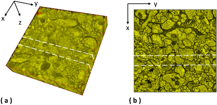
Two planes are randomly chosen for the ssTEM data of the drosophila melanogaster third instar larva ventral nerve cord to extract the side views of the 3D reconstructed objects generated by individual methods.

Serial section Transmission Electron Microscopy (ssTEM) of Droshophila brain

Two ssTEM image sets of the droshophila brain¹⁴,¹⁵ are tested in the experiments. The first one is released by Gerhard et al.¹⁴, containing 20 sections from serial section Transmission Electron Microscopy (ssTEM) of the Drosophila melanogaster third instar larva ventral nerve cord (VNC), which were freshly dissected and collected from instar fly brain. Every image is in the dimension of 1024 by 1024 pixel, with a resolution of 4.6 × 4.6 nm/pixel. The cube measures 4.7 × 4.7 × 1 microns approx, with section thickness of 45–50 nm. For this dataset, two planes are randomly chosen as shown in the Fig. 1 to extract the side views of the 3D reconstructed objects generated by individual methods, and the side views of the reconstructed objects by individual methods are presented in the Figs 2 and 3 respectively, showing that the proposed method produces solid 3D reconstructed objects with less discontinuity and deformation problems in comparison to the benchmark methods. For illustration purposes, red circles are marked to show that the proposed method yields a good continuity while some benchmark methods generate discontinued contours.

Figure 2. 1st side views of the reconstructed anatomical objects for the ssTEM data¹⁴.

Using the first plane chosen in Fig. 2, side views of the reconstructed anatomical objects by individual methods for the ssTEM data of the drosophila melanogaster third instar larva ventral nerve cord are displayed.

Figure 3. 2nd side views of the reconstructed anatomical objects for the ssTEM data¹⁴.

Using the second plane chosen in Fig. 2, side views of the reconstructed anatomical objects by individual methods for the ssTEM data of the drosophila melanogaster third instar larva ventral nerve cord are displayed.

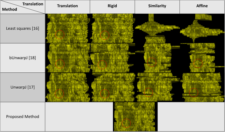
The second data set released by Cardona et al.⁹ contains 30 serial TEM sections of the drosophila first instar larval brain neuropile and one ventral nerve cord segment. Every image is in the dimension of 512 by 512 pixel, with resolution 4 nm/pixels and section thickness 50 nm. One plane as shown in Fig. 4 is randomly selected to extract the side views of reconstructed anatomical objects, and the side views of all objects are presented in Fig. 5, showing that the proposed method outperforms the benchmark approaches and yields a solid object with good continuity; a red circle highlights that the presented method align images well while the benchmark methods output more discontinuities. In addition, the fourth benchmark approach¹ fails to find corresponding features among sections and is not able to generate registration outputs.

Figure 4. Extraction of side views for the ssTEM data⁹.

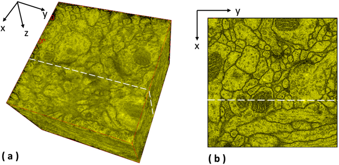
One plane is randomly selected for the ssTEM data of the drosophila first instar larva brain neuropile and one ventral nerve cord segment to extract the side views of the 3D reconstructed objects generated by individual methods.

Figure 5. Side views of the reconstructed anatomical objects for the ssTEM data⁹.

Side views of the reconstructed anatomical objects by individual methods for the ssTEM data of the drosophila first instar larval brain neuropile and one ventral nerve cord segment are displayed.

Serial histopathological images of renal cortical tissues

18 serial histopathological images of renal cortical tissues⁴ are used as the third test data. This data is comparably more challenging due to large variations on the data appearances, image orientation and size among sections, complex deformations and artifacts introduced during the data preparation process, causing existing methods fail to reconstruct a solid 3D object and perform poorly as shown in the Fig. 6. In addition, the fourth benchmark approach¹ fails to find corresponding features among sections and is not able to generate registration outputs. In comparison, the proposed method well aligns images in 3D and is still able to reconstruct a solid object with good continuity; the 3D reconstruction result is presented in the Fig. 7.

Figure 6. Side views of the reconstructed anatomical objects for the histopathological data⁴.

Side views of the reconstructed anatomical objects by individual methods for the histopathological data are displayed.

Figure 7. 3D reconstruction using serial histopathological microscopic images.

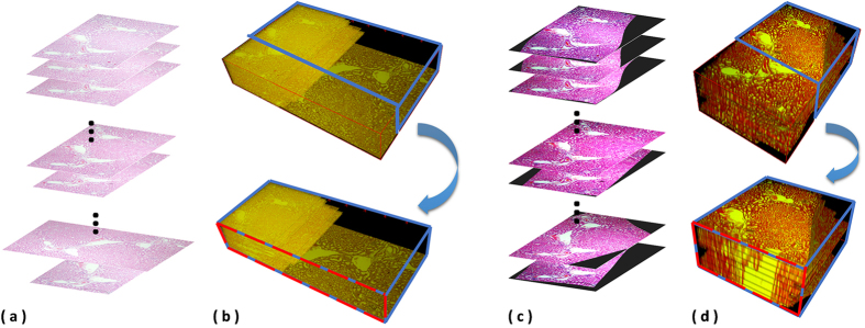
(a) the inputs for 3D registration are original serial histopathological images. Without registration, (b) serial images are sequentially placed into a 3D space, and a randomly selected plane can be defined to cut the 3D object into two parts. Then, the side view of the upper part object can be used to assess the continuity of the reconstructed 3D object. After registration by the proposed method, (c) registered images are sequentially placed in a 3D space to produce (d) a reconstructed 3D object.

Laser scanning microscopic images of the drosophila brain

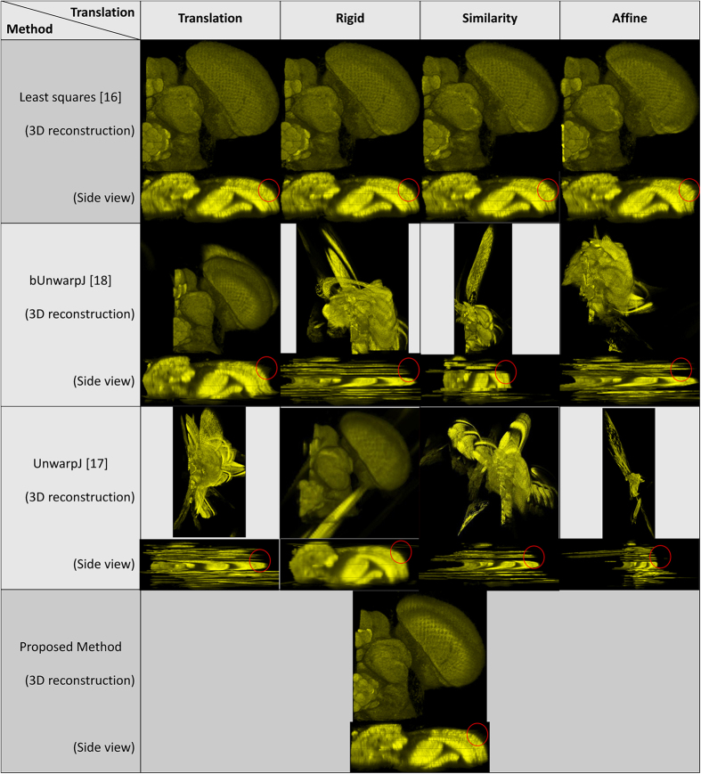
108 serial-section images of laser scanning microscopy of the drosophila brain is adopted as the fourth test set. This dataset is originally used to evaluate a 4D registration technology - BrainAligner by Peng et al.², which aligns pairs of 3D brain volumes. As shown in Fig. 8, a plane is randomly defined to extract side views of reconstructed anatomical objected by individual methods, and 3D reconstruction results with associated side views are presented in Fig. 9. Some of the benchmark approaches fail to produce solid 3D objects, and the fourth benchmark approach¹ fails to find corresponding features among sections and is not able to generate registration outputs. In comparison, the presented approach aligns images well in 3D and produces a solid object.

Figure 8. Extraction of side views for the laser scanning microscopic images of the drosophila brain².

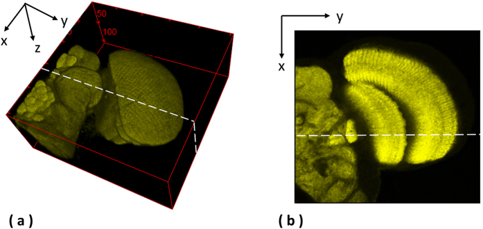
One plane is randomly selected for the laser scanning microscopic images of the drosophila brain to extract the side views of the 3D reconstructed objects generated by individual methods.

Figure 9. 3D reconstruction results with associated side views for the laser scanning microscopic images².

3D reconstruction results with associated side views of the 3D reconstructed objects generated by individual methods are presented for the laser scanning microscopic images of the drosophila brain².

Quantitative evaluation on a synthetic image sequence

For quantitative evaluation, a synthetic serial section test case is built by firstly creating a serial of ten identical images and secondly adding random deformation effects to individual images as shown in the Fig. 10. For the synthetic test case, a general registration performance measurement method, i.e. the percentage of pixels with similar intensity levels, is adopted to measure the registration accuracy, and an automatic evaluation tool is built to conduct quantitative evaluation automatically. Given a serial of images, , the overall registration accuracy, R, is formulated as the mean of the registration accuracies, r_i, of individual pairs, .

Figure 10. Synthetic image sequence for quantitative evaluation.

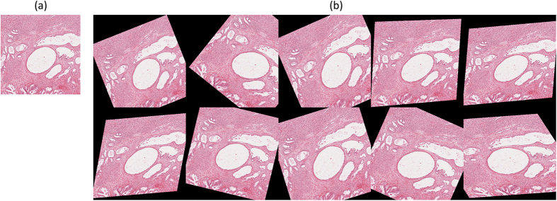
The synthetic image sequence is build by duplicating multiple biological tissue images as multiple sections and then applying random deformation effects to individual layers. (a) The tissue image to be duplicated. (b) The synthetic image sequence containing ten randomly deformed tissue images.

where and ; defines a mask common to the foreground Ω_i and Ω_i+1 of I_i and I_i+1; defines the foreground data after deformation, excluding the black background as shown in Fig. 10; defines the white pixels in the common area of I_i; t = 200 in our experiments.

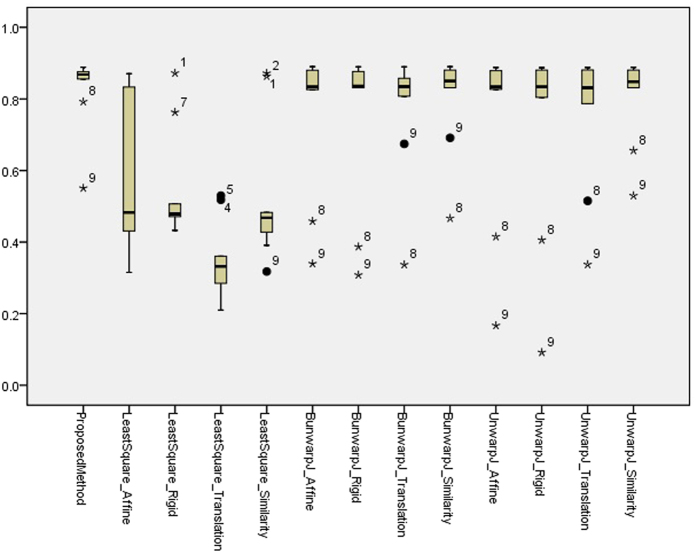
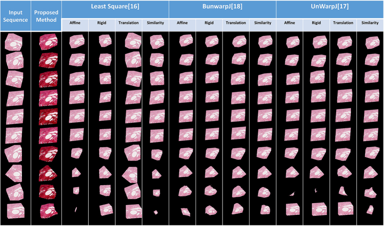
Table 1 presents the quantitative evaluation results, and the box plot of the quantitative evaluation results is provided in Fig. 11. Figure 12 presents the registration outputs of individual approaches. The experimental results shows that the proposed method achieves higher registration accuracy score and performs better than the benchmark approaches.

Table 1. Quantitative evaluation on the synthetic test case.

Method		Registration Accuracy (R)
Proposed Method		0.8268
Least Square16	Affine	0.6075
	Rigid	0.546
	Translation	0.347
	Similarity	0.5249
BunwarpJ18	Affine	0.756
	Rigid	0.7438
	Translation	0.7735
	Similarity	0.7978
UnwarpJ17	Affine	0.7299
	Rigid	0.7199
	Translation	0.7511
	Similarity	0.8026

^*Elastic method¹ fails in producing registration outputs.

Figure 11. A box plot of the quantitative evaluation results on the synthetic image sequence.

The presented methods works constantly well overall and outperforms the benchmark approaches. Outliers greater than 1.5× interquartile range (IQR) are marked with a dot, and outliers greater than 3 × IQR are marked with a asterisk.

Figure 12. Image Inputs and Registration outputs for the synthetic image sequence.

This figure shows the registration inputs and outputs by all methods for the synthetic test case.

Discussion

We have presented a robust and fully automatic 3D image registration technique for detailed anatomical reconstruction of serial-section microscopic images. The method is promising to reassemble continuous volumes and able to deal with complex distortions, staining variations and artifacts. We have demonstrated our method in application to four different microscopic image sets, including two serial ssTEM images, one laser scanning confocal image sequences and one serial histopathological images. The registration and reconstruction results show that the proposed 3D image registration method is robust and performs consistently well, even for data sets with large morphological distortion problems. The presented 3D image registration technique is not limited to tissue images but can also be applied to other anatomically or histologically defined medical data and will prove to be a substantial advantage for any application that requires 3D image registration. The software implementation of the presented method and the test data used in this study are made publicly available for scientific communities to use (http://www-o.ntust.edu.tw/~cweiwang/3DRegistration/).

Methods

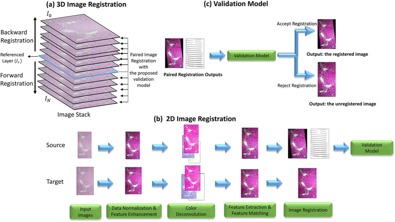
The proposed 3D image registration system combines and extends our recent efforts on robust 2D image registration⁴,⁵ and is devised with a new 3D alignment validation model utilizing the B-Spline deformation fields. The flowchart of the proposed method is shown in Fig. 13. Given the referenced layer I_r specified in this study), the proposed 3D registration conducts forward and backward image registration sequentially and bidirectionally for every two neighboring image pairs. The paired image registration consists of four steps: data normalization and feature enhancement, color deconvolution, feature matching and extraction, and image registration by using improved bi-directional elastic b-spline model. After the paired image registration is conducted to obtain an registered image with the associated deformation field, a validation model is applied by evaluating the deformation field. If accepted, the paired image registration output is as the final 3D registration result. Otherwise, the original image is used as the registration output. More details about each method can be found in the following subsections.

Figure 13. System framework of the proposed method.

Given the referenced layer I_r specified in this study), (a) the proposed 3D registration conducts forward and backward image registration sequentially and bidirectionally for every two neighboring image pairs. (b) The paired image registration consists of four steps: data normalization and feature enhancement, color deconvolution, feature matching and extraction, and image registration by using improved bi-directional elastic b-spline model. After the paired image registration is conducted to obtain an registered image with the associated deformation field, (c) a validation model is applied by evaluating the deformation field. If accepted, the paired image registration output is as the final 3D registration result. Otherwise, the original image is used as the registration output.

Data Normalization and Feature Extraction

The data normalization process is applied to reduce variations on image features and enhance tissue patterns. This greatly benefits global feature matching and local area-based directing matching processes as it automatically adjust the brightness and contrast of image color channels based on the image histogram distribution.

In color images, the value of each pixel is represented by a vector with elements the pixel values of each color component. Assuming a random vector, which models the pixel value for each color component in a color image. To exclude extreme pixel values, which may not be representative of the main image content, we saturate a fixed percentage at the upper and lower ends of the target intensity range where and are used in this work. The lower and the upper bound intensity levels of the histogram of each channel, x_low and x_high, are computed by the equations below. Given a histogram distribution H, where H(x) is the number of pixels with intensity level x, the lower and the upper bound values for transformation are formulated as follows.

where .

Next, it maps the original pixel value in the range from to to new value in the valid intensity scale from to .

The data normalization is proven to reduce stain variation and enhance tissue patterns, furthermore improving the following feature extraction model accuracy to identify valid corresponding control points⁴.

Our goal is to extract the eosinophilic structures, which are generally composed of intracellular or extracellular protein, as image features for image registration, and the color decomposition technique is utilized to extract independent haematoxylin and eosin stain contributions from individual histopathological images using orthonormal transformation of RGB.

In the RGB color-space, every color is defined as where r, g, b represent the red, green and blue components, and we can see additive color mixing as the vector addition of RGB components. To model the colors in an image as the vector addition of a desired (D) and undesired (U) components to a background color (P), new unit vectors can be defined as follows.

where is perpendicular to and ; , , span the 3D space; and are alternative unit vectors based on the undesired and desired colors.

Then, color can be transformed to the new unit vectors.

where ; is the origin in the RGB 3D space; is a vector.

By setting u = 0, we remove the undesired component and obtain the new color . In the case of three channels, the color system can be described as a matrix of the form with every row representing a specific stain and every column representing the optical density (OD) as detected by the red, green and blue channel for each stain.

For normalization, each OD vector is divided by its total length, such that (, and ). In this study, the normalized optical density (OD) matrix, , to describe the color system for orthonormal transformation is defined as follows:

when C is the 3 × 1 vector for amounts of the stains at a particular pixel, the vector of OD levels detected at that pixel is equal to . Therefore, multiplication of the OD image with the inverse of OD matrix results in orthogonal representation of the stains forming the image . Then, the image features of the red channel are extracted as eosinophilic structures for both high level feature-based coarse registration and local area-based direct matching registration.

2D image registration

Our proposed 3D image registration framework is based on our previous work,2D robust image registration⁴,⁵. In order to improve robustness, Our 2D image registration method incorporate two approaches: area-based and feature-based. Initially, sparse approximation for fast and coarse global registration is applied. Given I₁ and I₂ as two images for alignment, T as a set of all possible transformation between I₁ and I₂ and U_t(I) as the function that maps an image I to its transferred images using the transformation t, the goal is to find optimal transformation ⁵:

The transformation invariant distance corresponds to the regular Euclidean distance when the images are aligned optimally in L² where images are considered as continuous functions in , but finding the optimal transformation and the smallest distance d(I₁, I₂) is not easy as the objective function is non convex and local minima trap solution might occur. Feature based approaches represent a more efficient class of methods. Considered images can be well approximated by the sparse expansion in a series of geometric functions, we define as a set of geometric features constructed by transforming a generating function where represents a finite discretization of the transformations T and denotes the transformation of the generating function ψ by α. Given p and q as the respective K-sparse approximation of I₁ and I₂ in D,

where a_i, b_i are non-negative coefficients.

Then, the coarse global image registration problem can be formulated as finding the optimal relative transformation between the K-sparse approximations with the smallest approximate transformation invariant distance :

By utilizing the K-sparse approximations p and q are obtained by the previous procedures, and normalized image features F₁, F₂ from data normalization and feature extraction method, interested points S₁, S₂ can be detected by using the difference of Gaussian detector¹⁹ and then the corresponding feature points p, q are selected as geometric consensus between S₁ and S₂ using random sample consensus (RANSAC)²⁰. The selected paired feature points p, q are then used for coarse global registration.

After alignment outputs are obtained from the coarse global registration process, they will be refined by area-based direct-matching method which is adapted from the improved bi-directional elastic b-spline model¹⁸. The registration methodology is based on the minimization of an energy function that incorporates four energy terms:

where E_img is the energy of the similarity error between I₁ and , E_div, E_rot are the regularization energy based on the divergence and curl of the deformation, E_cons expresses the geometrical consistency between the elastic deformation in both direction , , and w_k are the weights for sub-energy terms).

3D Image Registration

In the proposed 3D image registration framework, 2D image registration is sequentially and bidirectionally conducted for every image with the neighboring sections. Given as a set of images to be aligned, as the set of registered images after 3D registration, I_r as the referenced image in this study), and Reg (S, T) as the 2D image registration function with S as the source image and T as the target image, a 3D image registration framework can be formulated as follow:

The aforementioned simple 3D framework however suffers from accumulated transformation errors or boosted over-deformation problems. When there are limited number of corresponding features detected or incorrect feature matching occurs, minor transformation error may be generated, and the transformation errors can be accumulated during the sequential registration process, causing over-deformed transformation results. Hence, in order to avoid over-deformation and accumulated transformation errors, we develop a validation model for the 3D registration framework. For every registration Reg (S, T), the validation model will automatically check if the transformation is valid or over-deformed. If valid, the 3D registration system will accept the transformation result as the 3D registration output .

A validation model using deformation fields for 3D registration

During image registration, deformation fields are produced to represent the geometrical distances generated by the transformation function. Mathematically, a forward deformation function can be defined as follows.

which means that this function transforms a two dimensional source image I_s, into an image as similar as possible to the two dimensional target image I_t. Here, the deformation fields are represented as a linear combination of B-splines, which can be formulated as follows.

where β³ is the B-Spline to the third degree, C_k,l are the B-Spline coefficients, and s_x and s_y are scalars that control the degree of detail of the representation of the deformation field.

A validation model is designed to automatically compute the average of geometrical distances using deformation fields. The system will reject the registration output, , when the average of geometrical distances is too large, which indicates that the transformation is over-deformed.

where α is a user-defined parameter that specifies the maximum of the mean deformation value to be allowed. Higher α value allows larger transformation but also allow higher accumulated transformation error, and hence over-deformations may occur with high α value. On the other hand, low α value may cause the validation model to reject a well-transformed registration output. Therefore, the α value should be low enough to reject over-deformed registration result and high enough to accept well-deformed registration. Table 2 shows the valid value range of the α value for individual datasets.

Table 2. α value range for each dataset.

Dataset	α value range
ssTEM Drosophila melanogaster third instar larva VNC14	20–200
ssTEM Drosophila melanogaster first instar larva VNC9	30–95
Serial histopathological images of renal cortical tissues4	200–350
Laser scanning microscopic images of the drosophila brain2	10–30

An illustration is given in Fig. 14 using the serial-section laser scanning microscope images of the drosophila brain data. (a) 3D reconstruction results with a side view of the raw input data are displayed; (b) an example of the backward registration from the image layer I₂₅ to the image layer I₂₃ is presented with associated deformation fields and validation processes. As the validation model accepts the deformation fields, , the outputs of the registration will be . On the other hand, is rejected by the validation model, and the registration output will be I₂₃. (c) Similarly, an example of the forward registration from Layer I₈₄ to the image layer I₈₆ is shown with associated deformation fields and validation processes. (d) 3D reconstruction results with a side view of the registered outputs are presented.

Figure 14. 3D image registration with the presented validation model.

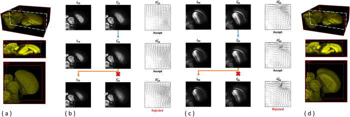
Using the serial-section laser scanning microscope images of the drosophila brain data as example, (a) 3D reconstruction results with a side view of the raw input data are displayed; (b) an example of the backward registration from the image layer I₂₅ to the image layer I₂₃ is presented with associated deformation fields and validation processes. As the validation model accepts the deformation fields, , the outputs of the registration will be . On the other hand, is rejected by the validation model, and the registration output will be I₂₃. (c) Similarly, an example of the forward registration from Layer I₈₄ to the image layer I₈₆ is shown with associated deformation fields and validation processes. (d) 3D reconstruction results with a side view of the registered outputs are presented.

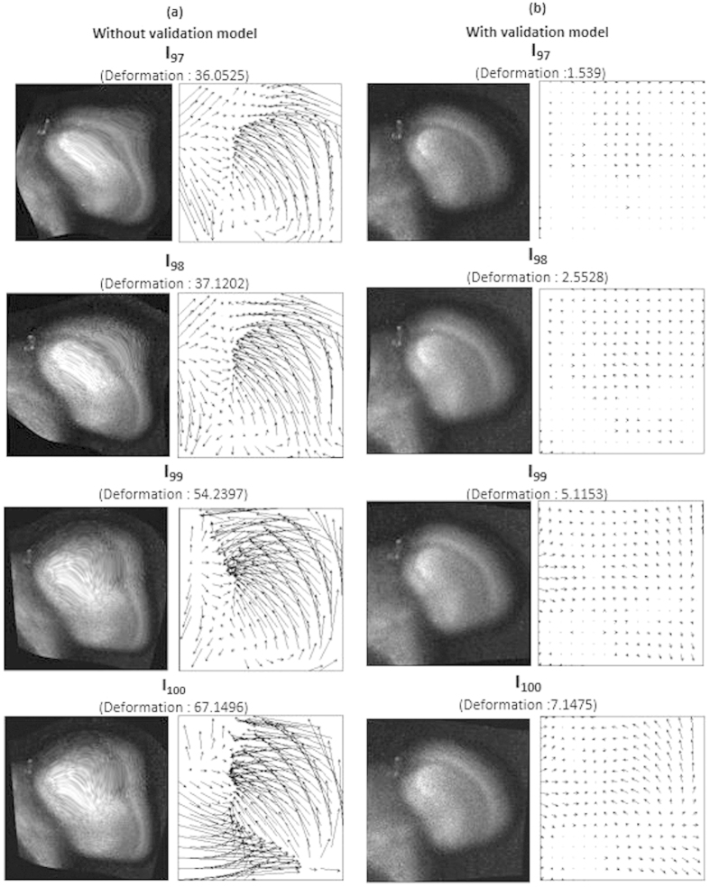
The validation model ensures that the accumulated over-deformation error does not proceed and affect the rest of the registration process. Figure 15 compares the registration results with associated deformation fields with and without the proposed validation model, showing that the registration results without the presented validation model suffers from over-deformation problems and accumulates transformation errors. Over-transformed registration outputs accumulate the transformation errors, causing higher transformation error in the registration process of the next layer.

Figure 15. Compare the registration outputs with and without the validation model.

This figure compares the registration outputs (a) without the validation model and (b) with the validation model applied, showing that the registration results without the presented validation model suffers from over-deformation problems and accumulates transformation errors. Over-transformed registration outputs accumulate the transformation errors, causing higher transformation error in the registration process of the next layer.

Data and Software

The software implementation of the presented method is developed in JAVA (with jdk 1.7.0.51 installed) and based on Fiji framework¹⁶ and TrakEM2 image registration framework⁹. The software and the data are both made publicly available for scientific communities to use (http://www-o.ntust.edu.tw/~cweiwang/3Dregistration/).

Additional Information

How to cite this article: Wang, C.-W. et al. Fully automatic and robust 3D registration of serial-section microscopic images. Sci. Rep. 5, 15051; doi: 10.1038/srep15051 (2015).

References

- Saalfeld S., Fetter R., Cardona A. & Tomancak P. Elastic volume reconstruction from series of ultra-thin microscopy sections. Nat. Methods 9, 717–720 (2012). [DOI] [PubMed] [Google Scholar]
- Peng H., Ruan Z., Long F., Simpson J. H. & Myers E. W. V3d enables real-time 3d visualization and quantitative analysis of large-scale biological image data sets. Nat Biotech 28, 348–353 (2010). [DOI] [PMC free article] [PubMed] [Google Scholar]
- Peng H. et al. BrainAligner: 3D registration atlases of Drosophila brains. Nat. Methods 8, 493–498 (2011). [DOI] [PMC free article] [PubMed] [Google Scholar]
- Wang C.-W., Ka S.-M. & Chen A. Robust image registration of biological microscopic images. Sci. Rep. 4, 10.1038/srep06050 (2014). [DOI] [PMC free article] [PubMed] [Google Scholar]
- Wang C.-W. & Chen H.-C. Improved image alignment method in application to x-ray images and biological images. Bioinfo. 29, 1879–1887 (2013). [DOI] [PubMed] [Google Scholar]
- Fiala J. C. Reconstruct: a free editor for serial section microscopy. J. Microscopy 218, 52–61 (2005). [DOI] [PubMed] [Google Scholar]
- Saalfeld S., Cardona A., Hartenstein V. & Tomancak P. As-rigid-as-possible mosaicking and serial section registration of large ssTEM datasets. Bioinfo. 26, i57–i63 (2010). [DOI] [PMC free article] [PubMed] [Google Scholar]
- Cardona A. et al. An Integrated Micro- and Macroarchitectural Analysis of the Drosophila Brain by Computer-Assisted Serial Section Electron Microscopy. PLoS Biology 8, e1000502 (2010). [DOI] [PMC free article] [PubMed] [Google Scholar]
- Cardona A. et al. TrakEM2 Software for Neural Circuit Reconstruction. PLoS ONE 7, e38011 (2012). [DOI] [PMC free article] [PubMed] [Google Scholar]
- Chakravarty M. et al. The creation of a brain atlas for image guided neurosurgery using serial histological data. NeuroImage 30, 359–376 (2006). [DOI] [PubMed] [Google Scholar]
- Dauguet J. et al. Three-dimensional reconstruction of stained histological slices and 3D non-linear registration with in-vivo MRI for whole baboon brain. Kidney Int. 164, 191–204 (2007). [DOI] [PubMed] [Google Scholar]
- Tan Y., Hua J. & Dong M. 3D reconstruction from 2D images with hierarchical continuous simplices. Visual Comput. 23, 905–914 (2007) [Google Scholar]
- Pitiot A. & Guimond A. Geometrical regularization of displacement fields for histological image registration. Med. Image Anal. 12, 16–25 (2008). [DOI] [PubMed] [Google Scholar]
- Gerhard S., Funke J., Martel J., Cardona A. & Fetter R. Segmented anisotropic ssTEM dataset of neural tissue (2013). URL http://dx.doi.org/10.6084/m9.figshare.856713.
- Cardona A. et al. An integrated micro- and macroarchitectural analysis of the drosophila brain by computer-assisted serial section electron microscopy. PLoS Biol 8, e1000502 (2010). URL http://dx.doi.org/10.1371. [DOI] [PMC free article] [PubMed] [Google Scholar]
- Schindelin J. et al. Fiji: an open-source platform for biological-image analysis. Nat Meth 9, 676–682 (2012). [DOI] [PMC free article] [PubMed] [Google Scholar]
- Sorzano C., Thevenaz P. & Unser M. Elastic Registration of Biological Images using Vector-Spline Regularization. IEEE Trans. Biomed. Engin. 52, 652–663 (2005). [DOI] [PubMed] [Google Scholar]
- Arganda-Carreras I. et al. Consistent and Elastic Registration of Histological Sections using Vector-Spline Regularization. LNCS, Comput. Vis. Approaches to Med. Imag. Anal. 4241, 85–95 (2006). [Google Scholar]
- Lowe D. Distinctive Image Features from Scale-Invariant Keypoints. International Journal of Computer Vision 60(2), 91–110 (2004). [Google Scholar]
- Fischler M., Bolles R. Random Sample Consensus: A Paradigm for Model Fitting with Applications to Image Analysis and Automated Cartography. Comm. of the ACM 24(6), 381–395 (1981). [Google Scholar]