Spike timing precision changes with spike rate adaptation in the owl's auditory space map

Abstract

Spike rate adaptation (SRA) is a continuing change of responsiveness to ongoing stimuli, which is ubiquitous across species and levels of sensory systems. Under SRA, auditory responses to constant stimuli change over time, relaxing toward a long-term rate often over multiple timescales. With more variable stimuli, SRA causes the dependence of spike rate on sound pressure level to shift toward the mean level of recent stimulus history. A model based on subtractive adaptation (Benda J, Hennig RM. J Comput Neurosci 24: 113–136, 2008) shows that changes in spike rate and level dependence are mechanistically linked. Space-specific neurons in the barn owl's midbrain, when recorded under ketamine-diazepam anesthesia, showed these classical characteristics of SRA, while at the same time exhibiting changes in spike timing precision. Abrupt level increases of sinusoidally amplitude-modulated (SAM) noise initially led to spiking at higher rates with lower temporal precision. Spike rate and precision relaxed toward their long-term values with a time course similar to SRA, results that were also replicated by the subtractive model. Stimuli whose amplitude modulations (AMs) were not synchronous across carrier frequency evoked spikes in response to stimulus envelopes of a particular shape, characterized by the spectrotemporal receptive field (STRF). Again, abrupt stimulus level changes initially disrupted the temporal precision of spiking, which then relaxed along with SRA. We suggest that shifts in latency associated with stimulus level changes may differ between carrier frequency bands and underlie decreased spike precision. Thus SRA is manifest not simply as a change in spike rate but also as a change in the temporal precision of spiking.

the temporal structure of sound carries important information allowing for its identification and categorization as well as for many aspects of communication. A wide variety of species can discriminate between vocalizations almost entirely on the basis of temporal envelope structure (e.g., Brenowitz 1983; Gerhardt and Bee 2006; May et al. 1989; Pollack and Hoy 1981). Humans, for example, can comprehend degraded speech sounds as long as the patterns of amplitude modulation (AM) are left intact (see, e.g., Shannon et al. 1995).

Given the ethological importance of temporal structure, it is not surprising that neurons in various auditory centers fire in precise synchrony with a sound's amplitude envelope (see, e.g., Rokem et al. 2006; Zheng and Escabi 2013). Neurons of the auditory nerve and cochlear nucleus will phase lock to periodic envelopes up to and above 1 kHz (see, e.g., Joris and Yin 1992; Kim et al. 1990; Rhode and Greenberg 1994; Steinberg and Pena 2011), and midbrain neurons will phase lock up to several hundred hertz (Keller and Takahashi 2000; Krishna and Semple 2000; Rees and Møller 1987). Neurons will also fire in synchrony to envelope segments of aperiodic sounds that have a specific shape characterized by the cell's spectrotemporal receptive field (STRF) (see, e.g., Frisina et al. 1990; Heil and Irvine 1997; Joris and Yin 1992; Kayser et al. 2010; Moller 1974; Swarbrick and Whitfield 1972). Neurons of the barn owl's midbrain space map both are sensitive to the spatial location of sound sources and fire selectively for particular envelope shapes, marking their occurrences with tightly phase-locked spikes (Keller and Takahashi 2000). These neurons thus carry necessary information for both sound localization and identification.

Spike rate adaptation (SRA) is a continuing change of a neuron's sensitivity to ongoing stimuli. Traditionally, SRA was most often characterized in response to a constant stimulus. A neuron's poststimulus time histogram (PSTH) shows an initial, often high, firing rate that relaxes over time toward a long-term rate, which is usually lower. Responses of space map neurons generally follow this pattern with a strong burst of activity that diminishes sharply over the next few hundred milliseconds.

The sensitivity of auditory neurons to stimulus amplitudes is traditionally quantified by plotting the firing rate, averaged over the course of a stimulus, against the stimulus level, generating the rate-level function (RLF). In nature, the average ambient sound level can fluctuate over a wide range, and the sensitivity of a neuron to its inputs adapts continuously (Benda and Hennig 2008; Gutfreund and Knudsen 2006; Harris and Dallos 1979; Kiang 1966; Pumphrey 1936; Smith 1979). RLFs of midbrain auditory neurons have been shown to shift along the x-axis with changes in the distribution of the stimulus levels presented, thus allowing the dynamic range of the neuron to move toward the mean of the stimulus's amplitude distribution (Benda and Hennig 2008; Dean et al. 2005, 2008; Rees and Palmer 1989).

Synchronization to the envelope of sinusoidally amplitude-modulated (SAM) noise is strongest with stimuli having an average amplitude near to, or slightly above, the area of the RLF's maximal slope (Cooper et al. 1993; Smith and Bachman 1980; Yates 1987). An abrupt increase in sound pressure level (SPL) may initially place a neuron near saturation on its RLF, thus inducing vigorous but less envelope-synchronized firing. As the neuron adapts, SRA may cause the RLF to shift and the spike rate to drop. The cell's envelope synchrony should improve with a similar time course. Our study sought evidence for this prediction and attempted to characterize the link between SRA and envelope synchrony more mechanistically. We first demonstrate the phenomenon of SRA and the shift of the RLF in space map neurons. A model of continuous adaptation (Benda and Hennig 2008; Benda and Herz 2003) is shown to explain the shift of the cells' RLFs, thus mechanistically linking SRA to the RLF shifts. The model is based on the idea of an “effective stimulus,” I_eff(t), which is the momentary SPL minus the degree to which the neuron has adapted. We next show that spike timing to SAMs immediately following a sudden increase in stimulus level is initially imprecise but then improves with a time course similar to that of SRA. Similarly, the spike rate output of the model, driven by the I_eff(t), showed initially degraded temporal locking, which then improved with a similar time course. Finally, we demonstrate that changing neural synchrony observed with SAMs generalizes to more naturalistic stimuli having aperiodic envelopes. We used the idea of a neuron's STRF, which characterizes a neuron's selectivity for specific envelope shapes, to estimate the precision of individual spikes. We could thus assess the relative timing of individual spikes with even a single stimulus presentation. Studies in other systems have often reported changes in the STRF following sudden changes in mean stimulus amplitude (Dean et al. 2005; Kvale and Schreiner 2004; Lesica and Grothe 2008a; Nagel and Doupe 2006; Shechter and Depirieux 2007). In our study, the spike-triggered average (STA) stimulus, used to estimate the STRF, was also found to change with the stimulus. Recalculation of the STA with the I_eff(t) and correcting for changing spike timing precision (dejittering), however, made it clear that the STRF itself remained constant and only the jitter-contaminated STAs changed. We conclude that adaptation maintains the ability of space map neurons to lock precisely to amplitude fluctuations against a background of changing mean amplitude.

METHODS

All procedures were performed under a protocol approved by the Institutional Animal Care and Use Committee of the University of Oregon.

Surgical procedures.

Recordings were obtained from nine captive-bred adult barn owls (Tyto alba) anesthetized by intramuscular injection of ketamine (KetaVed, 0.1 ml at 100 mg/ml or ∼22.5 mg/kg; Vedco) and Valium (diazepam, 0.08 ml at 5 mg/ml or ∼0.9 mg/kg; Abbott Laboratories, Abbott Park, IL) as needed (approximately every 3 h). Each bird was fit with a headplate for stabilization within a stereotaxic device and also with bilateral recording wells through which electrodes were inserted (Euston and Takahashi 2002; Spezio and Takahashi 2003).

Stimulus generation and experimental procedures.

Stimulus construction and data analysis were performed in MATLAB (R2010a–R2012b, MathWorks, Natick, MA). All stimuli were synthesized digitally at a sampling rate of 30,000 points/s. Sounds were filtered through individualized head-related impulse responses (HRIRs) that were recorded and processed as described by Keller et al. (1998) (5° resolution, double polar coordinates). Stimuli were convolved in real time with location-specific HRIRs [Tucker Davis Technologies (TDT), Alachua, FL; PD1], convolved again with inverse filters for the earphones, attenuated (TDT PA4), and impedance matched (TDT HB1) to a pair of in-ear earphones (ER-1; Etymotic Research, Elk Grove Village, IL).

Stimuli.

The basic stimulus was a broadband noise (BBN) presented near the center of the cell's spatial receptive field (SRF) and constructed as the inverse Fourier transform of unitary amplitude and random phase spectra between 2 and 11 kHz. The stimulus had 5-ms-duration linear onset and offset ramps. These stimuli were used in two experimental paradigms based on the work of Dean and colleagues (2005) and of Nagel and Doupe (2006).

Paradigm modified from Dean et al. (2005).

This paradigm was used to test whether RLFs of space map neurons adapt to changes in the stimulus distribution. RLFs were generated by repeating a 32-s BBN whose SPL changed every 50 ms (see Fig. 4A, green bars). For each 50-ms epoch, the SPL was randomly drawn with replacement from a rectangular probability density function (PDF) of levels spanning 31 dB in 1-dB increments. These distributions are shown, inverted, along the y-axis in Fig. 4A and along the x-axis of Fig. 4B. The central 11 levels of the PDF comprised a “high-probability region” with 80% of the total available values. These high-probability SPLs are represented by the solid green bars in Fig. 4A, which exemplifies the paradigm for a PDF with a mean at 20 dB SPL. The dashed green bars in Fig. 4A show the outliers comprising the remaining 20% of the total available values. Additional RLFs (differing colors in Fig. 4B) were obtained by shifting the entire PDF along the x-axis so that the RLFs could be assessed at different mean SPLs. Each stimulus repetition used a newly randomized drawing of levels from the PDF and new instantiations of both the carrier and the envelope unless otherwise noted. Spikes were assigned to a particular epoch after subtraction of an overall latency, and average firing rates for each stimulus level were obtained.

Fig. 4.

RLFs shift toward the high-probability region of the stimulus distribution. A: each stimulus repetition consisted of six hundred 50-ms epochs of broadband noise whose intensity (green lines) was randomly drawn for each epoch from a rectangular distribution of levels (shown to left of y-axis). Dotted green lines indicate stimulus levels outside the high-probability region comprising 80% of the level values. B: spike rate responses obtained for 6 different stimulus distributions (stimulus histogram outlines reflected about x-axis) are shown in differing colors for 1 neuron. Mean neuronal responses to the high- and low-probability stimulus regions (±SE) are shown along with output from the model (heavy solid lines). Highest stimulus intensity curve for the model (red) is shown both without (thin lines) the divisive spike rate limiting parameter, α, and with (thick lines) α and a 3-dB decrease in stimulus intensity. Dotted red lines indicate the differences between these 2 curves. Estimated neuronal thresholds (Benda and Hennig 2008) are indicated by inverted arrowheads. C and D: estimated thresholds plotted against the mean of the high-probability portion of the stimulus distribution for this cell (C) and for a sample of 30 cells (D). The regression line and a 1-to-1 line are shown for comparison. E and F: maximum slope (spikes·s⁻¹·dB⁻¹) of the Boltzmann fit to the neuronal data for this cell (E) and for the sample of cells (F). G and H: maximum spike rate (spikes/s) is plotted against the shift in estimated threshold for this cell (G) and for the sample of cells (H). Data for the cell in B are shown in red in the population plots (D, F, H).

The paradigm above was modified to examine the effect of adaptation on the spike timing precision to SAM noise. The unmodulated noise in each 50-ms epoch was replaced with SAM noises (see Fig. 6L) having a modulation frequency of 100 Hz, resulting in 5 SAM cycles per epoch (modulation depth = 75%). Phase locking to the SAM noises was quantified by computing the vector strength (VS; Goldberg and Brown 1969). VS, which is the magnitude of the Rayleigh vector, ranges between 0 and 1, where VS = 1 indicates that neurons discharge with perfect synchrony to the SAM envelope.

Fig. 6.

Neuronal and model responses to sinusoidally amplitude-modulated (SAM) noise. A, B, D, and E: raster plots: SPL of the signal before modulation is given on y-axis and color-coded using red for the highest SPL. A and B: responses during the 1st (A) and 5th (last) (B) amplitude modulation (AM) cycles for epochs with an increase in stimulus level from the previous epoch. D and E: equivalent plots for epochs with a decrease in stimulus level. C: vector strengths (VSs) plotted against the AM cycle number for epochs following an increase in SPL (color coding reflects SPL as in A and B). F: VSs following SPL decreases. Data obtained from 1 cell with 10 repetitions of the 30-s stimulus. VSs calculated for SPLs occurring at least 40 times (in 6,000 total epochs) and AM cycles eliciting at least 10 spikes (19,437 spikes total). G and J: firing rates estimated with the model (Benda and Herz 2003) for level increases (G) and decreases (J). The temporal pattern of AM is indicated by the gray sinusoidal line. Responses averaged over 60 instantiations of a 30-s stimulus. H and K: VSs for stimuli shown in G and I, respectively (same color coding as in A–F) for each AM cycle. Data shown only for SPLs occurring in at least 40 of the total 36,000 epochs. The high-probability region of stimulus level is marked by the gray brackets on the y-axes (A, B, D, E, G, and J). I: VS from the 3rd AM cycle vs. VS from the 1st cycle for 9 cells for selected SPLs (indicated by the color scheme used in A–F). Diagonal black line indicates no change of VS between cycles. Data for individual cells connected by lines (dotted line indicates cell from A–F). L: the stimulus paradigm is the same as shown in Fig. 4, except that each 50-ms epoch consisted of SAM noise (75% modulation depth). Since the modulation frequency is 100 Hz, there are 5 cycles per epoch.

Paradigm modified from Nagel and Doupe (2006).

We employed two versions of this paradigm to test for adaptive changes in stimulus filtering. Each version presented 10–50 repetitions of a 30-s-duration BBN. In the first version, there were four 7.5-s-long epochs with envelopes having the following characteristics, in order: 1) low mean (∼20–30 dB above neuronal threshold), low variance [interquartile range (IQR) = 1.3 dB]; 2) low mean (but +2.8 dB above the level of epochs 1 and 3), high variance (IQR = 4.4 dB); 3) low mean, low variance (repeat of epoch 1); 4) high mean (+9.6 dB above the level of epoch 1 or 3), low variance (IQR = 1.3 dB). The present analysis looks only at the low- and high-mean epochs (epochs 3 and 4). In the second version, the four epochs alternated between the low and high mean always with the same low variance. For each stimulus version, we constructed a stimulus with a duration of 7.5 s. To minimize across-frequency correlations, stimuli were built as sums of gammatone-filtered BBNs (center frequencies from 1 to 11 kHz, in 100-Hz increments; Slaney 1993). For each center frequency, an envelope was created having a uniform magnitude spectrum below 100 Hz and a cross-covariance coefficient with envelopes of adjacent frequency bands of <0.5. Envelopes were scaled in magnitude and variance for each of the four stimulus epochs and multiplied by the filtered BBNs. The four epochs were then concatenated to form one 30-s-long stimulus. No differences were discernible between the responses to either stimulus version, and these results are thus presented together.

Initial characterization of neurons.

All recordings were carried out in a sound-isolating booth (Industrial Acoustics, 1.8 m × 1.8 m × 1.8 m). Extracellular single-unit recordings were made with tungsten microelectrodes (Frederick Haer, Brunswick, ME). We recorded units with well-restricted SRF and relatively broad frequency tuning as occur in both the lateral shell and external subdivisions of the inferior colliculus (ICcls and ICx, subsequently referred to as ICx) and do not distinguish between the two histological subdivisions. Spike times were recorded to computer disk at a resolution of 10 μs (M110; Modular Instruments). Cellular responses were first characterized by varying interaural level difference (ILD), interaural time difference (ITD), and level by frequency-independent adjustments of the signals to each ear. To estimate a cell's SRF, we measured responses to stimuli presented sequentially from location-specific HRIRs forming a checkerboard pattern across the frontal hemisphere. Stimuli for further testing were presented through HRIRs corresponding to a location near the center of each cell's SRF. The vast majority of cells in our sample had highly restricted SRFs centered within ∼20° of the center of gaze and had best frequencies (BFs) between 3.5 and 9 kHz.

Continuous adaptation model.

Benda and Herz (2003) developed a phenomenological model to explain SRA based on the idea of an I_eff(t). To compute I_eff(t), the model subtracts the cell's momentary level of adaptation, A(t), from the applied stimulus intensity, I(t):

$${\text{I}}_{\text{eff}}\left(t\right)=\text{I}\left(t\right)-\text{A}\left(t\right)$$ (1)

The model posits no specific mechanism of adaptation or of spike generation but assumes the spike rate, R(t), to be directly proportional to the magnitude of I_eff (in dB), thus:

$$\text{R}\left(t\right)\propto \left[\text{I}\left(t\right)-\text{A}\left(t\right)\right]$$ (2)

Figure 1 illustrates the derivation of A(t) from the maximum adaptation available, A_max. For a given stimulus level, A_max is defined by the shapes of two versions of a neuron's RLF. RLF₀(I) (Fig. 1A; blue sigmoid) gives the neuron's initial response to varying levels of stimulation from a completely unadapted state. RLF_∞(I) (Fig. 1A; red sigmoid) depicts the “fully adapted” response after prolonged stimulation at each stimulus level. A_max is the difference in SPLs that generate the same spike rate on RLF₀ and RLF_∞. For example, a stimulus intensity of 10 dB elicited ∼4 spikes/s on average from the fully adapted neuron (Fig. 1A; red RLF at +10 dB). When the neuron was completely unadapted, however, an SPL of only −5 dB was sufficient to elicit the same response. A_max is the intensity difference for eliciting similar responses from these two neuronal states, or, in this case, ∼15 dB (length of double-headed arrow labeled b in Fig. 1A).

Fig. 1.

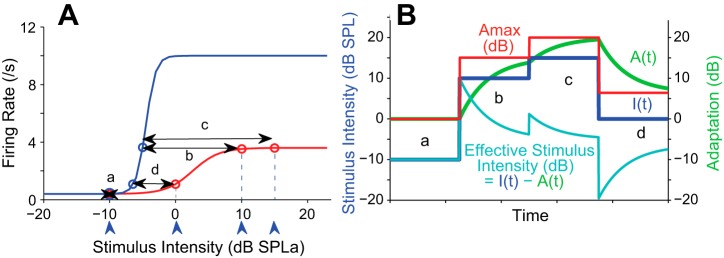
Continuous adaptation model (Benda and Herz 2003) A: sigmoidal fits to each rate-level function (RLF) for a representative inferior colliculus (ICx) neuron. RLF₀ was obtained when the neuron was unadapted (blue) and RLF_∞ when the neuron was fully adapted (red). The maximum possible adaptation (A_max) is calculated from the difference between these 2 curves as a function of stimulus intensity [length of double-headed arrows (a–d) for each of 4 stimulus intensities, blue arrowheads]. B: a period of stimulation over which the stimulus intensity, I(t), changes over 4 different values (dark blue line, left y-axis, levels a–d from A). A_max, calculated in A, is plotted in red and referenced to the right y-axis scale. The actual moment-by-moment adaptation [A(t), green, right y-axis] is calculated by a relaxation from the current level toward A_max. The resulting effective stimulus intensity (cyan, left y-axis) is the difference of the input stimulus intensity less adaptation, thus: I_eff(t) = I(t) − A(t).

For most natural stimuli the intensity is always changing. Figure 1B presents four moments in time (epochs a–d) over which the presented stimulus intensity, I(t), changes as shown by the dark blue lines. These SPLs correspond to the blue arrowheads below the x-axis in Fig. 1A. Whereas the increments and decrements in I(t) resemble those from the stimulus paradigm of Dean et al., the timescale is determined either by the rate at which the stimulus changes or, conversely, by the time window over which the neuron integrates the stimulus. As the stimulus changes, so too does A_max (red line in Fig. 1B). A neuron's level of adaptation, A(t) (green line in Fig. 1B), has units of intensity and relaxes from its current state toward A_max with a time course derived from the neuron's PSTH. At the start of epoch b, adaptation is 0 dB but begins to increase toward A_max (= 15 dB). When the time constant is long relative to the epoch duration, adaptation does not quite reach A_max before A_max is shifted to a new value by the change in stimulus intensity (epoch c). Thus some of the history of the stimulus is retained within the current level of adaptation. Faster adaptation loses this history; slower adaptation retains more history.

In Fig. 1B, the effective stimulus intensity, I_eff(t), (cyan line) equals the applied stimulus intensity, I(t), (blue line) minus the momentary level of adaptation, A(t), (Eq. 1; green line). Thus A(t) can be either greater than or less than A_max, forcing adaptation to either increase or decrease with time and thus shifting the RLF to either the right or the left, respectively. Thus at each point in time the effect of adaptation on the rate-intensity curve depends upon both A_max(t) and the history of stimulation embodied within A(t).

Although not critical to the interpretation of our findings, additional stimulus level-related changes to the RLF, beyond the left/right shifts induced by a subtractive current, may also apply. To accommodate these changes, and following the procedures of Benda and Hennig (2008), a “divisive” term, α, was included in the model, thus:

$$\text{R}\left(t\right)\propto \left[\text{I}\left(t\right)-\text{A}\left(t\right)\right]/\alpha$$ (3)

This limits the maximum rate at higher SPLs and decreases the slope as the curve shifts to the right.

We implemented the model with a sampling interval of 30 kHz. Separate exponential time constants for adaptation and for recovery from adaptation were allowed and chosen by inspection of the direction of change of the stimulus level, I(t), at each time point. For calculation of the I_eff(t) and prediction of the PSTH, the ongoing level of adaptation derived by the model was scaled to match the PSTH and subtracted from the applied stimulus. We obtained RLF₀, RLF_∞, and RLF_a (described below) curves from 52 neurons using stimuli patterned after those of Benda and Hennig (2008). For RLF₀ and RLF_∞, responses were gathered from 10 or more repetitions of 33-s-long BBNs divided into 1.5-s epochs. The intensity of each epoch alternated between 20 dB or more below threshold and various suprathreshold levels. Each epoch's ending firing rate (F_∞) was calculated as the mean rate in the last 100 ms of the epoch. The initial firing rate (F₀) was the rate in the 1-ms time bin with the maximum difference from the previous epoch's F_∞. RLF_a curves represent the initial responses of neurons in an adapted state (denoted by stimulus level “a” in the subscript). Stimuli for collection of these data alternated 1,500-ms adapting epochs at a given stimulus level with 100-ms test epochs at various levels. We calculated the relative reduction in maximum firing as a function of adaptation strength from RLF_a curves as described in Benda and Hennig (2008). RLF_a curves derived in this manner are strongly similar to RLFs derived from the stimulus paradigm modified from Dean et al. (2005), described above. In many neurons, adapted firing rates were very low, resulting in nearly flat and near-zero RLF_∞ curves. This made calculation of A_max indeterminate (Fig. 1), and therefore we parameterized the model using smoothed curves from one cell that was typical of cells with a rising RLF_∞ curve (Fig. 1). We estimated the time courses of adaptation and recovery from exponential or power-law fits to changes in firing rate for long-duration stimuli (see results). This may underestimate actual time constants of adaptation if, for example, maximal adaptation is set by the (changing) firing rate and not by the (constant) stimulus (Benda et al. 2005; Benda and Herz 2003).

Exponential [R(t) = factor × e^(−t/τ) + constant] and power-law [R(t) = factor × t^−α + constant] fits to the neuronal PSTH were obtained with the MATLAB “fit” function using the “NonlinearLeastSquares” method. We report “adjusted R²” values (adjR²) to adjust for the number of variables in the calculation. For analysis of model responses to SAM stimuli, estimated firing rates in 1-ms time bins were used to weight unit vectors that were then combined into the Raleigh vector for calculation of VS.

Estimation of spectrotemporal receptive field.

The STRF represents the filtering properties of a neuron and thus determines the way in which a neuron will respond to amplitude-modulated stimuli. The STRF is estimated by computing the STA, which is simply an average spectrogram of the sound preceding each spike.

To compute the STA, a broadband stimulus was passed through a bank of 81 evenly spaced gammatone filters (Slaney 1993; center frequencies between 2 and 10 kHz). Each frequency band represents the output of a gammatone filter approximating the owl's auditory nerve tuning curves (Köppl 1997). The envelope of each spectral band was then extracted as the time-varying magnitude of the Hilbert transform, which could be plotted as a function of frequency and time (e.g., Fig. 2A). The STA was calculated by averaging these stimulus spectrograms for the 15-ms segment immediately preceding each spike, less an equivalent number of spectrograms from randomly chosen 15-ms segments. The resulting STA was normalized by its Frobenius norm:

$$\text{Frobenius norm}=\sqrt{{\displaystyle {\sum }_{t=-15}^0{\displaystyle {\sum }_{f=2,000}^{10,000}{\left(\text{spectrogram element}\right)}_{tf}^2}}}$$ (4)

Fig. 2.

Estimation of jitter. A: spectrogram of the stimulus preceding a spike. x- and y-axes represent, respectively, the time before a spike and the carrier frequencies (81 bands). Warm colors represent high envelope amplitudes. B: spike-triggered average (STA). Stimulus spectrograms preceding each spike (occurring between 2 and 7.5 s after the transition to the high-mean stimulus) were averaged to generate the STA. The offset of the STA's peak (red) from 0 ms represents the average latency across all spikes. STRF, spectrotemporal receptive field. C and D: for each spike, the cross-covariance between the STA and prespike spectrogram was calculated for each of 11 frequency bands surrounding the best frequency (BF) of the STA. N spikes were obtained during the presentation of an epoch; results from the 1st spike (C) and from the Nth spike (D) are shown in separate panels. Within each frequency band, we use the location of the peak of the cross-covariance to calculate the difference in latency vs. the average latency of the STA (“added delay,” black asterisks and black downward arrows). From the 11 latencies for each spike, we compute a median added delay (gray asterisks, gray downward dashed arrows) and the variation about this median [calculated as their interquartile range (IQR) demarked by the black brackets]. This variation is the jitter in latencies across frequency bands for a given spike and is called the “between-frequencies jitter.” For the cross-covariance function shown in C, the median latency across the 11 frequency bands is shorter than the average latency represented by the STA and therefore the median added delay is negative. Each spike's median added delay can also be accumulated into a distribution of N samples (gray bracket). The IQR of this distribution is called the “between-spikes jitter” and represents the precision of spike times relative to the STA. Inset, color scale used in C and D.

Thus the STA provides an estimate of the shape of the average prespike signal at each carrier frequency and prespike time. The frequency band containing the peak of the STA was designated as the cell's “best frequency” (BF). The time from the peak of the STA to 0 ms gave the average spike latency within each frequency band.

The match between a particular 15-ms stimulus fragment with the STA was quantified by projecting the fragment's envelope spectrogram onto the STA using the matrix dot product. The distribution of all projections from a given stimulus epoch, calculated for each millisecond of the stimulus, is called the “prior” and represents a null hypothesis for neuronal selectivity. “Spike-eliciting” projections normalized to the mean and standard deviation of the prior are thus “z scores” relative to the null hypothesis.

Calculation of individual spike delay.

Stimuli used to examine spike timing precision in response to naturalistic stimuli (Nagel and Doupe 2006) have complex envelopes that produce modulation patterns that may differ across carrier frequency bands. We used the temporal relationship between each spike-eliciting envelope (Fig. 2A) and the STA (Fig. 2B) to estimate the relative timing of each spike. The STA and each spike-eliciting envelope comprise matrices with 450 time steps × 81 frequency bands. Since we know only approximately which band(s) actually triggered a spike, we computed the cross-covariance (Fig. 2, C and D) of the STA and the envelope segment preceding the spike in each of 11 frequency bands surrounding a cell's BF (centers at BF ± 500 Hz). In each frequency band, the time lag at the maximum of the cross-covariance gave an estimate of the difference in latency (“added delay”) for a given spike relative to the average latency obtained from the STA. An added delay of 0 ms indicates that the spike's latency was equal to the latency of the STA within that band (added delay = 0). Because we used 11 frequency bands, there were 11 added delays for each spike (black asterisks and small downward arrows, Fig. 2, C and D). The dispersion of these 11 values for each spike, calculated as their IQR, is called the “between-frequencies jitter” (black brackets, Fig. 2, C and D). Between-frequencies jitter reflects how well the temporal alignment of spike-eliciting envelope segments matches the alignment seen in the STA. The median of the 11 added delays (gray asterisks, gray dashed arrows in Fig. 2, C and D) was also calculated for each spike. Calculating the median added delay using 21 frequency bands or calculating a weighted average using the height of the cross-covariance peak as weight had no discernible effect on our results. For a response giving N spikes, there will be N median values of added delay. The IQR of these N median values provides a measure of the temporal precision between spikes and is called the “between-spikes jitter” (Fig. 2D; gray bracket). Between-spikes jitter is analogous to measures of spike timing variability reported in other studies (e.g., Mainen and Sejnowski 1995). However, as opposed to most earlier studies, our use of the STA as a timing reference allows us to compare timing both within and across stimuli without having to repeat stimuli.

RESULTS

We report data from single neurons recorded from the ICx and ICcls (collectively referred to as ICx) of nine barn owls under ketamine-valium anesthesia.

Spike rate adaptation.

All cells showed strong SRA similar to the classic descriptions of Kiang (1966), Smith (1979), and Harris and Dallos (1979) recording from the auditory nerve. A portion of the response to a constant-intensity 2,000-ms noise burst for one exemplary neuron is shown in Fig. 3A. An initially robust response declined rapidly to a very low spike rate. The decline in firing frequency was well fit by a single exponential with a time constant (τ_a) of ∼23 ms (adjR² = 0.89). For most cells, the decay could be fit with a power law with equal or better adjR². The power-law exponent (α) estimated for the response shown in Fig. 3A was 0.55 (adjR² = 0.85). Since our stimuli covered only a small range of timescales, our analysis was not affected by the choice of exponential or power-law decay (Fairhall et al. 2001).

Fig. 3.

Spike rate adaptation and recovery in the ICx. A: poststimulus time histogram of response for 1 ICx neuron to a broadband noise burst (dashed line, exponential fit; dotted line: power-law fit, over 2,000 ms; 55 stimulus repetitions). adjR², adjusted R² value. B and C: recovery of firing rate (B) and first-spike latency (C) measured by responses to test noise bursts presented at various intervals after offset of the 2,000-ms conditioning noise burst. Each response curve was fit with an exponential (dashed gray lines) and a power law (dotted gray lines). D–G compare the estimated fit parameters for recovery plotted against the equivalent values for adaptation for 18 ICx neurons. D and F show spike rate; E and G show spike latency. Open circles indicate values for the neuron depicted in A–C. Unity slope line is drawn for comparison.

When the applied stimulus, I(t), decreased, the cell's firing first declined and then recovered, generally recovering with a longer time constant than observed for responses to increasing I(t). We estimated time constants for recovery with an initial 2,000-ms conditioning noise followed at various intervals by a 100-ms test noise (Fig. 3B). Values fit to the recovery of the cell shown in Fig. 3 were τ_r = 121 ms and α_r = 0.24. Other authors have inferred from similar data that different mechanisms may apply for adaptation and recovery from adaptation (e.g., Chimento and Schreiner 1991; Fairhall et al. 2001; Ingham and McAlpine 2004). Full recovery to the initial spike rate occurred only over seconds (not shown). First-spike latency to the test pulses recovered more rapidly than the spike rate (Fig. 3C; τ_r = 36 ms; α_r = 0.16). Figure 3 shows these estimated adaptation and recovery time constants (Fig. 3, D and E) and power-law exponents (Fig. 3, F and G) measured from 18 cells.

Rate-level functions shift with adaptation.

Using the stimulus paradigm of Dean et al. (2005) (methods), we tested cells with a broadband stimulus whose level changed every 50 ms (Fig. 4A) and was picked from a prescribed distribution of levels, shown reflected along the x-axis in Fig. 4B. With such stimuli, adaptation resulted in a shift of the RLF toward the mean of the stimulus intensity distribution. As the stimulus distribution was moved to higher intensities (e.g., cyan → blue → green → red, Fig. 4B), the RLF and the neuronal threshold (colored triangles, Fig. 4B) shifted rightward (Fig. 4, C and D). As the curves shifted to the right, both their maximum slope and maximum spike rate diminished (Fig. 4, E and G), resulting in a slightly increased range of stimuli over which the cell's response rate changes.

A continuously updated I_eff(t) (Fig. 1B) can replicate these shifts in the neuronal RLFs (Benda and Hennig 2008). When the distribution of stimulus levels was shifted, the RLFs predicted by the model shifted to the right or left in similar fashion as the neuronal curves (Fig. 4B, thick lines). To generate these plots, we calculated A_max(t) using responses of the unadapted and fully adapted neurons (methods; Fig. 1A) and a time constant of 100 ms. Just as in the neuronal responses, leftward shifts (Fig. 4B, gray and black curves) are limited by the neuron's threshold in the unadapted state. Additionally, the model has a difficult time predicting responses near the lower limits of the applied stimulus, where both the adapted and unadapted curves are relatively flat and maximal adaptation, A_max, is thus ill-defined.

Rightward shifts of neuronal RLFs were usually accompanied by a decrease in the maximum rate and a decrease in the curve's slope that were not replicated by the purely subtractive model (compare thin red line and filled circles in Fig. 4B). Adding a divisive term to the model (for calculation, see α in Benda and Hennig 2008; Eq. 3) limits the maximum rate at higher SPLs and decreases the slope as the curve shifts to the right. It was beyond the aims of the project to explore the ultimate limits to the rightward shift of neuronal responses, but shifts in response to the most intense stimuli tested were of lesser magnitude than shifts near the middle of the range. Thus for Fig. 4 we lowered the input intensities of the highest-level stimuli to the model by 3 dB to better match the neuronal output. To demonstrate the necessary adjustments to the model at higher stimulus levels, the model's output for this test before and after these two adjustments are shown in red in Fig. 4B, with red dotted arrows to indicate the resultant shifts in the curves.

The RLFs showed large adaptive shifts when the neuron was presented with a stimulus whose distribution shifted from low SPLs (Fig. 5A; regime 1, 0–5 dB SPL; right y-axis) to high SPLs (regime 2, 16–21 dB SPL). These shifts were closely predicted by the I_eff(t) (Fig. 5, C–F). Figure 5 shows that A_max, the maximum available adaptation (Fig. 5A, gray, right y-axis), changed with each epoch and jumped sharply at the onset of the second regime. Adaptation, A(t) (Fig. 5A, blue, left y-axis), increased or decreased toward A_max, thus continuously shifting the I_eff(t) (Fig. 5B, right y-axis). The model's predicted firing rate closely tracked actual neuronal firing (Fig. 5B, black, left y-axis), demonstrating that adaptation to the new regime (regime 2; Fig. 5) is a continuous process and differs only in magnitude from adaptation to each new epoch.

Fig. 5.

Neuronal and model responses to a change from low to high stimulus intensities. A: stimulus level (green bars, right y-axis) changes from 0–5 dB (regime 1) to 16–24 dB SPL (regime 2). A_max (gray trace, left y-axis) changes rapidly, driving the (smoothed) change in adaptation (blue, left y-axis). B: the effective stimulus intensity, I_eff(t) (green trace, right y-axis), is tracked closely by the neuronal firing rate (black trace, left y-axis). C and D: spike rate as a function of time when the regime changes from low to high (green) and high to low (red) for an ICx neuron (C) and the model (D; stimuli different from that in A). E and F: RLFs for each regime for the neuron (E) and model (F). Outline of histogram of stimulus level distribution shown for each regime (gray rectangles).

Adaptation of the spike rates for both the neuron and the model were manifest in a complete shift of the RLF (Fig. 5, E and F). Thus for these neurons continuous subtractive adaptation coupled with a rate-limiting divisive component (Benda and Herz 2003) can fully account for the dynamics of shifting RLFs. Adaptation of the RLF to the stimulus mean is a manifestation of ongoing subtractive SRA (Benda and Hennig 2008) and is analogous to RLF shifts seen in other animals.

The RLF is an indicator of neuronal sensitivity obtained from spike rates averaged over a period of constant stimulus intensity. We next modified the stimulus to probe the effects of SRA on spike timing in response to a continuously changing stimulus intensity.

Precision of spike locking to stimulus envelope improves during adaptation.

Space map neurons, as with most auditory neurons, can be strongly driven by AMs of the stimulus envelope and will strongly phase lock to SAMs up to ∼200 Hz (Keller and Takahashi 2000). We examined the effects of adaptation on envelope phase locking with a modified version of the Dean et al. (2005) stimulus paradigm. For each 50-ms epoch, we multiplied the stimulus with a 100-Hz sinusoidal envelope, resulting in 5 modulation cycles per epoch having a modulation depth of 75% (Fig. 6L). We estimated the degree of phase locking for the response to each AM cycle by calculating the VS (Goldberg and Brown 1969).

Figure 6, A–F, depict the responses of a typical cell having a high VS. Figure 6, A–C, show responses evoked when the SPL of an epoch is increased from that of the previous epoch. Spiking is shown as raster plots for the first and last AM cycles of the epoch (Fig. 6, A and B, respectively). The SPLs of the epochs (before modulation) are displayed along the y-axis and each raster is color-coded, with red corresponding to the highest SPLs. Each SPL is presented multiple times over the course of the stimulus (see Fig. 6 legend), and the occurrences of all spikes across all presentations of a given stimulus condition are condensed into a single raster line. Gray brackets to the right of the y-axes demarcate the high-probability region of the stimulus distribution. Figure 6C plots the VS against cycle number using the same color coding to indicate the SPL of the epoch. Figure 6, D–F, show corresponding data for decreases in SPL.

Spike rates after level increases adapted strongly between the first (Fig. 6A) and last (Fig. 6B) AM cycles. The reduction in spike number was accompanied by improving temporal precision (increasing VS), most apparently for the highest stimulus levels and more gradually for lower SPLs that fell within the high-probability region of the stimulus. The change in envelope locking with cycle number is more easily seen in Fig. 6C, which plots VS against cycle number. Note that VS is lowest in the first cycle and for the epochs with the highest SPL. In other words, increases of mean level to the highest SPLs are most deleterious to envelope locking. These are also, on average, the largest level increases. However, continuous adaptation over the epoch allows the cell to recover its ability to phase lock to the SAM. The VS is less affected when the increases in SPL are more modest but still shows recovery through the last AM cycle. Very few spikes occurred at the lowest SPLs, making it difficult to compute a reliable VS. Although the 50-ms epoch may not allow complete recovery of the VS, by the last AM cycle VS remains slightly higher for SPLs within the high-probability region. Spike latency was also increased at the lower SPLs, as is apparent by the rightward shift of the rasters with the cooler colors (Fig. 6B).

Data are summarized for nine cells in Fig. 6I, which plots the VS obtained in the third cycle against the VS obtained in the first cycle after an increase of I(t). (Many cells produced insufficient spikes for calculation of VS in the 4th and 5th cycles.) The color of each filled circle in Fig. 6I represents the magnitude of the SPL, and data from a given cell are connected by thin lines; the heavy black diagonal has a slope of 1 (VS_1st = VS_3rd). As shown, nearly all cells show an improvement of VS by the third cycle.

Spiking responses to decreases of stimulus level (Fig. 6, D–F) were accompanied by an increase in spike rate but little change in VS between the first and last AM cycles. VS became somewhat more uniform across SPLs by the last cycle. Thus SRA, manifested as spike rate changes within an epoch, was accompanied by systematic changes in spike timing and the precision of envelope phase locking.

The I_eff(t) can explain both SRA and the accompanying changes in spike timing and spike timing precision as shown in the lower two rows of Fig. 6. In Fig. 6, G and J, the firing rates computed from the model are shown for increases and decreases, respectively, in SPL. The VS computed from the predicted firing rate is plotted against cycle number in Fig. 6, H and K. For stimulus level increases (Fig. 6G), firing was strongest and broadest in time for the first AM cycle and became gradually weaker and narrower in successive cycles. Modeled and observed responses behaved similarly, as can be seen by comparing Fig. 6, H and C. In Fig. 6H, the VS is lowest during the first AM cycle, especially for the higher amplitudes (warmer colors), and increases on successive cycles. By the fifth cycle, the outputs of both the cell and the model near a plateau, with higher SPLs showing slightly lower VSs.

As was observed in the cell (Fig. 6F), for stimulus decreases the model shows no or only slight increases in VS with cycle number at intermediate SPLs (Fig. 6K). Note that the model, which does not include a spike generator to give spike times, allows VS to be computed from the predicted spike rate even for SPLs that evoked few if any spikes in the neuron. Therefore, Fig. 6K displays results from lower SPLs (yellow and light green) additional to those shown in Fig. 6F.

Responses to complex envelopes.

The VS measure allows us to estimate spike timing precision from the firing rate or from the model's effective stimulus averaged over repetitions of the AM cycle (see methods), but it does not allow us to measure the temporal precision of individual spikes to ongoing, changing stimuli. Furthermore, deeply modulated SAM stimuli cause synchronous modulation in all carrier frequency bands, and although they elicit robust responses from space map neurons, it is unclear whether the timing of these responses can be extrapolated to spike timing precision to more complex aperiodic envelopes such as may be encountered in nature.

We now use a stimulus paradigm similar to that of Nagel and Doupe (2006) (methods; inset above Fig. 7E) to ask whether similar results apply to the temporal precision of individual spikes obtained in response to sounds with more complex envelope features. Given such stimuli, space map neurons are selective for envelope segments of a particular shape that matches the cell's STRF (Fig. 2B; Keller and Takahashi 2000). The STRF cannot be known exactly but can be estimated as the spike-triggered average stimulus spectrogram (STA). We examined the timing of individual spikes by comparing the timing of envelope segments preceding each spike (Fig. 2A) with their timing in the STA (estimated from late in the high-mean stimuli). Using the STA as the temporal reference allows us to compare spike timing within and across stimuli without requiring repetition of the same stimulus. Our analysis is based on responses of 72 neurons presented with broadband stimuli that increased in intensity by 10 dB between two sequential 7,500-ms epochs (“low-mean” → “high-mean”).

Fig. 7.

Spike timing in response to an increase in stimulus level as shown in inset above E. A: added delay calculated from the cross-covariance between the STA and the spike-eliciting stimulus envelope. Each gray dot represents the median added delay for spikes occurring within a 1-ms time window, combined across stimulus repetitions and across cells. Probability density function (PDFs) (black lines) show the distributions of these values accumulated for each 500 ms. Added delay equals 0 when the individual spike's latency is the same as the average latency seen in the STA. After the stimulus level increase, added delay is initially negative (to left of 0), indicating spike latency is shorter than for the STA but relaxes toward 0 (dashed line) over 100 s of ms (rightward shift of the PDFs). For each 1-ms time bin, the median added delay across spikes was calculated for each cell, and the median across cells is plotted as a gray dot (n = 5–36 cells/dot). B: PDFs of spike latency relative to the STRF for spikes occurring early (gray) and late (black) in the 7,500-ms epoch. C: between-frequencies jitter (IQR across 11 frequencies for each spike). The IQR of added delays across frequencies was calculated for each spike, and the median of this value was calculated for each time bin for each cell. The median across cells was then calculated and plotted for each time bin as in A. Between-frequencies jitter was initially high after the SPL increase and relaxed toward a long-term value (dashed line) over hundreds of milliseconds (leftward shift of PDFs). D: PDFs of between-spikes jitter from spikes occurring early (gray) and late (black) in the epoch. E and F: between-spikes jitter as a function of time for the first 2 s after the increase in stimulus level (note break in time axis). E: data for 1 neuron; gray dots as in A. F: data averaged over 36 cells (n = 5–36 cells per point). Gray horizontal line is the long-term average; dashed gray line is the power-law fit.

The average “latency” of responses to spike-eliciting envelope segments is the time lag of the positive peak of the STA (see methods). The latencies of individual spikes jitter about this mean, and we refer to this as “between-spikes jitter” (Fig. 2D, gray bracket). Additionally, spike latency from an envelope segment may differ across frequency bands and the probability of spiking is highest when the envelope segments, and hence latencies, line up as they are aligned in the STA. The degree of misalignment relative to the STA is referred to as “between-frequencies jitter” (Fig. 2, C and D, black brackets).

As with the SAM stimuli, spike latency was initially shorter and more variable immediately after onset of the high-mean epoch and became longer and more precise over time. Figure 7A shows the change in spike latencies from the start of the high-mean epoch. Gray dots represent the median cross-covariance delay (“added delay”) for individual spikes averaged across cells (see Fig. 7 legend). Added delays were initially negative, indicating that spike latencies were initially shorter than the average latency (Fig. 7A, dashed vertical line) embodied in the STAs. PDFs for every 500 ms of data are overlaid and clearly show a rightward shift (lengthening latency) with time after the epoch onset, closely approaching the average latency within less than a second. Figure 7B shows early (16–515 ms) and long-term (2,000–7,500 ms) PDFs of the added delays relative to the STA, averaged across cells. The gradual increase in latency after the onset of the high-mean stimuli is highlighted with a gray arrow in Fig. 7B.

The initially short and gradually lengthening spike latencies were not equivalent across frequencies. In Fig. 7C, gray dots represent the median across cells of the IQR of the added delays across frequencies, a measure of between-frequencies jitter. For the high-mean stimuli, an initially high variability between frequency bands gave way to tighter between-frequencies alignment (a leftward shift of the histograms in Fig. 7, C and D). In other words, for early spikes, spike-eliciting envelopes matched the STA better in some frequency bands than in others, but for spikes occurring later in the epoch latencies were more like those of the STA across all frequency bands considered.

Overall spike timing was also less precise (between-spikes jitter was high) immediately after the stimulus level increase and improved toward its long-term value with a time course similar to that of SRA. Figure 7, E and F, show the between-spikes jitter during the first 2 s after the transition from the low- to high-mean stimuli. Results are shown for a single exemplary neuron (Fig. 7E) and averaged across 36 cells (Fig. 7F). The between-spikes jitter for each cell was estimated across stimulus repetitions within 1-ms time bins, and these estimates were then averaged across cells. The long-term average jitter is shown for comparison (Fig. 7, E and F, gray line).

Thus there are two types of spike timing jitter, each of which increases immediately with the increase in stimulus level and then more gradually relaxes toward its long-term value over a time course similar to that of SRA.

Spike jitter changes the STA but not the STRF.

A number of authors have suggested that neuronal filters change with adaptation (see discussion). Changes in spike timing precision may explain such observations. A neuron's intrinsic filtering properties, i.e., the STRF, are estimated with the STA. The STA, however, is a convolution of the distribution of spike timing with the STRF (Gollisch 2006) and thus is influenced by spike timing precision. Even for a neuron that is highly selective for a particular envelope shape, the optimal envelope waveforms will be misaligned during averaging, resulting in a broader STA and a shallower selectivity function (Gollisch 2006). These effects increase as jitter time increases (Aldworth et al. 2005). Therefore, as temporal precision improves with adaptation, the STA should become sharper in time and may change shape in other ways with no change in the underlying neuronal filter.

We examined these effects by recalculating the STA after “dejittering” the stimulus envelope segments for each spike. To dejitter, we added each spike's median added delay to the recorded spike time before extraction of the spike-eliciting stimulus fragment from the effective stimulus and recompilation of the STA (Aldworth et al. 2005; Chang et al. 2005; Dimitrov and Gedeon 2006). Example STAs, before and after dejittering for one ICx neuron, are shown in Fig. 8, A–D. As expected and as can be seen by comparing Fig. 8, A and B (low-mean stimulus) or C and D (high-mean stimulus), dejittering made the STAs for each neuron temporally sharper (note the red contour lines). Moreover, the dejittered STA showed no change in shape over the duration of a 7,500-ms stimulus epoch or after the transition from low-mean to high-mean epochs. Figure 8, E–G, show average temporal cross sections through the peak of the STA for a particular time window after the transition from low mean to high mean (as, for example, along the solid line crossing the peak of the STA in Fig. 8D). Each cross section represents an average across the STAs of 22 neurons after first normalizing their peak height and shifting their peak latency to coincide. The top three curves of Fig. 8E depict average cross sections before dejittering (left y-axis). STAs computed from early spikes (15-2,000 ms after the transition) initially showed a leading negativity that diminished over time (2,000–4,000 ms, 4,000–6,000 ms). The bottom three curves of Fig. 8E (right y-axis) were calculated after dejittering and lie completely atop one another, thus demonstrating that, although the STAs changed during SRA, the underlying STRF did not. Overlaying cross sections before and after dejittering for early spikes (Fig. 8F) and for late spikes (Fig. 8G) makes it clear that, by minimizing the variance in spike times, dejittering eliminates the leading negativity and temporally sharpens the STA. Thus improved spike timing in the course of SRA in effect “dejitters” the estimated STA.

Fig. 8.

A–D: spike-triggered average spectrograms (STAs) for the low-mean (A and B) and high-mean (C and D) epochs for 1 ICx neuron: STAs calculated with the applied stimulus, I(t), before (A and C) and after (B and D) dejittering. Each STA was constructed from 3,990 spikes chosen randomly from those occurring at least 2,000 ms after epoch onset over 20 stimulus repetitions. Each STA was normalized to its Frobenius norm (Eq. 4). Linear color scale applies to each panel. Contour lines are shown for z scores of ±3, 4, and 5 from the background level. Bootstrapped coefficients of cross-covariance within and between STAs (subscripts denote epoch numbers, dejittered in parentheses): XCov_3,3 = 0.81 (0.94), XCov_4,4 = 0.72 (0.92), XCov_3,4 = 0.71 (0.82). E: temporal cross sections through the BF (as, e.g., along the solid black line in D), averaged across STAs obtained from the high-mean epoch for 22 cells. Each STA was normalized to its peak height and shifted in time for the peaks to coincide before averaging. Plots representing STAs computed in 3 different time frames are shown before dejittering (top plots, left y-axis) and after dejittering (bottom plots, closely overlaid, right y-axis). Arrow emphasizes changes in the leading negativity between time frames. F and G: averaged cross sections before and after dejittering are redrawn for the early (F; 15-2,000 ms) and late (G; 4,000–6,000 ms) time frames.

Neuronal selectivity for the degree of match between the STA and the stimulus envelope also appeared to change between stimulus levels and through the course of SRA (not shown). The degree of matching was estimated as the projection of the STA onto each envelope fragment. To allow comparison across differing stimuli and spike rates, we normalized the projections for spike-eliciting envelope fragments to the distribution of all projections across all envelope fragments for a given stimulus (see methods). Selectivity curves showing a neuron's firing rate as a function of this normalized projection appeared to steepen with increasing time after the transition from the low-mean to high-mean stimulus. However, dejittering the STAs used for these estimations also eliminated the apparent change in the selectivity function. Thus neither the underlying neuronal filter nor the neuron's selectivity for the filter appears to change under our stimulus conditions; only their jitter-contaminated estimates do.

SRA changes dependence of spike jitter on the match between envelope fragments and the STA.

The precision of spike timing was strongly dependent upon the normalized projection, which quantifies the match of the spike-eliciting envelope fragment with the STA. This relationship is shown for between-frequencies jitter in Fig. 9A and for between-spikes jitter in Fig. 9B. Envelope fragments having higher projection values better match the STA and elicited spikes with higher temporal precision. The curves for the low-mean and high-mean stimuli are indistinguishable. However, immediately after the transition from low to high mean, the curves were initially flattened (Fig. 9, dashed blue lines). The steep slope recovered over time until the high-mean and low-mean curves again became indistinguishable. Most notably, between-spikes jitter decreased strongly over time in response to envelope fragments with high projection values, whereas jitter changed little at low projection values. Thus the strengthening of temporal fidelity to envelope fragments that best match the neuronal filter appears to be the primary mechanism of jitter reduction over time.

Fig. 9.

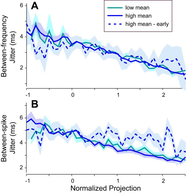
Relationship between spike timing jitter and projection: average across 36 cells of between-frequencies (A) and between-spikes (B) jitter plotted against the normalized projection value, a measure of the similarity between the spike-eliciting envelope and the STA. Spike-eliciting envelope fragments that more closely match the STA have higher projection values and lower jitter for both the high- and low-mean epochs (see key). Jitter for high projection values increased after the transition from the low- to high-mean stimulus (dashed dark blue line), but recovered to the previous low value as the high-mean stimulus continued. For each cell, average values were calculated across spikes that were sorted into bins of normalized projection value. Plots show averages (lines) and SE (shading) across cells (n = 5–36 cells per point) for early spikes (dashed; 10–110 ms after epoch onset) and late spikes (solid; 2,500–7,500 ms after epoch onset).

DISCUSSION

For neurons of the barn owl's ICx, SRA is a continuous process that drives the RLF to the left or right and is closely allied with continuous changes in spike timing. Upon a rapid increment in stimulus level, the neuron initially responds according to the RLF associated with the previous lower stimulus level, all the while moving its RLF progressively rightward as SRA proceeds. The neuron is momentarily “more sensitive” to the stimulus than it would be if fully adapted, responding at shorter latency and with lowered temporal fidelity. As adaptation proceeds, the spike rate diminishes, spike latency lengthens, and spiking becomes more temporally precise. Initially, temporal precision depends only weakly on the strength of the match between the envelope segment and the STRF. As SRA proceeds, envelope segments that more closely resemble the STRF elicit spiking that is more strongly stimulus locked.

Translation of the RLF along the level axis is a defining characteristic of subtractive adaptation as exemplified by the model of Benda and Herz (2003). The model (Benda and Hennig 2008), and our own results, emphasize that this “adaptation to stimulus statistics” is simply a manifestation of continuing adaptation and recovery. RLFs shift at various levels of the auditory system, and right/left shifts seem to be strongest at higher processing levels (see, e.g., Alves-Pinto et al. 2010; Costalupes et al. 1984; Dean et al. 2005; Gibson et al. 1985; Nagle and Doupe 2006; Rees and Palmer 1989; Watkins and Barbour 2011; Wen et al. 2009). These effects may occur over many timescales and may result from a number of candidate subtractive currents (see, e.g., Benda et al. 2010; Prescott and Sejnowski 2008).

In the barn owl's ICx, translations of the RLF are accompanied by gradual changes in RLF shape. Higher stimulus levels are associated with shallower RLF slopes (lower “gain”) and with lower maximum firing rates. Evidence from the auditory systems of other species suggests that changes in gain and maximal firing may be separable from shifts in the RLF (see, e.g., Gibson et al. 1985; Watkins and Barbour 2008; Wen et al. 2009). These shape changes require the addition of a “divisive” component to the model (Benda and Herz 2003). Mechanisms underlying divisive processes might include synaptic depression (Abbott et al. 1997; Chance et al. 2002; David et al. 2009; David and Shamma 2013; Tsodyks and Markram 1997) and adaptive thresholds (see, e.g., Azouz and Gray 2000; Ferragamo and Oertel 2002; Howard and Rubel 2010; Pena and Konishi 2002). Adaptive thresholds are also known to support precise spike timing over a wide range of stimulus levels (Fontaine et al. 2013; Geis and Borst 2009; Higgs and Spain 2011; Platkiewicz and Brette 2011), so adding a variable spike threshold to the basic subtractive model might serve to both change the shape of the RLF and account for changes in spike timing precision (Benda et al. 2010).

SRA and responses to SAMs.

A role for adaptation in shaping the responses of neurons to SAM stimuli is suggested by several earlier studies (see, e.g., Bibikov 2008, 2013; Rees and Palmer 1989; Smith and Brachman 1980, 1982). When SAM sounds are presented, the firing of midbrain and lower-order neurons is modulated in synchrony with the envelope modulation (reviewed by Joris et al. 2004). These and other authors have used the idea of “modulation gain” to quantify the depth of response modulation relative to the depth of the SAM, analogous to our measure of VS. Modulation gain is a peaked function of SPL predictable from the shape of the RLF (Cooper et al. 1993; Joris and Yin 1992; Smith and Brachman 1980; Yates 1987). Neuronal firing is modulated as the SPL of the stimulus traverses the RLF. Thus one expects the highest modulation gain, and the highest VS, to fall at SPLs corresponding to the steepest part of the RLF. However, the actual peak location and shape of the modulation gain function depends also on the depth and frequency of modulation as well as the processing level in the auditory system (see, e.g., Rees and Palmer 1989).

Deviations from the expected position of the gain function might largely be explained by adaptation on various timescales. For example, modulation gain functions obtained from cochlear nerve fibers in response to SAM frequencies of several hundred hertz and modulation depths of 35% (i.e., modulations of about ±3 dB) have their peak shifted rightward (to higher SPLs) and fall off more slowly than expected at higher SPLs (Smith and Brachman 1980, 1982). These SAM frequencies fall within the 1–2 ms timescale of the so-called “rapid” adaptation of the synapse between the hair cell and the auditory nerve. RLFs obtained from only the first 2 ms of auditory nerve fiber responses are steeper and saturate more slowly with increasing SPL and thus allow more accurate prediction of the observed modulation gain function (Smith and Brachman 1982).

We found that adaptation over tens of milliseconds allows recovery of phase locking to the envelope after an abrupt increase in stimulus level. Recovery coincides with a decrease in the I_eff(t), which also drives the shift in the RLF. For our stimuli, an abrupt increase in stimulus level immediately placed the mean stimulus level far to the right along the RLF and elicited a high firing rate. The 75% modulation depth on a decibel scale, however, causes the SPL to fluctuate between about 12 dB below and 5 dB above the mean level. This sweep across the RLF caused the neuronal response to be phase locked, but not as tightly as one would expect if the SAM was more centered on the steepest portion of the RLF. Over tens of milliseconds, however, the mean of the I_eff(t) decreased toward the steepest slope region. The firing level decreased and VS increased. In other words, adaptation preserved the neuron's dynamic range for phase locking.

The model suggests that differing timescales of adaptation should lead to both RLF shifts and VS recovery at a rate corresponding to the adaptation time constant. Adaptation on timescales from tens of milliseconds to seconds gives similar results. For example, neurons in the brain stem auditory nuclei of the frog show both SRA and recovery of modulation gain over several seconds (Bibikov 2008, 2013). On very short timescales, the results of Smith and Brachman (1982) suggest a resonance of adaptation and SAMs with high modulation frequencies that lead to gain amplification and other changes in the shape of the modulation gain function. Similar effects at longer timescales have not been examined.

SRA and responses to complex envelopes.

While the SAM stimuli allowed reconstruction of spike rates and their temporal modulation by the effective stimulus, neither the SAMs nor the subtractive model (Benda and Herz 2003) provides insight into actual spike timing on the scale of individual spikes. By looking at spike timing relative to the cell's preferred stimulus envelope, estimated with the STA, we found that SRA operates at the level of individual spikes as well and that spike timing precision improves over the course of an epoch with a time course similar to SRA.

A number of studies have reported stimulus level-dependent differences in the STRF, which imply changes in the stimulus-filtering properties of a neuron. For instance, higher stimulus levels have been associated with a more biphasic STRF, having a deepened leading negativity, thus making the cell more closely approximate a band-pass filter (see, e.g., Fontaine et al. 2014; Krishna and Semple 2000; Lesica and Grothe 2008b; Miller et al. 2002; Nagel and Doupe 2006; Valentine and Eggermont 2004). Changes in the STRF have also been described from in vitro experiments on first-order neurons in the chick's time coding pathway (Higgs et al. 2012; Kuznetsova et al. 2008). In these neurons, sustained depolarization elicits an increased spike rate, where these “newly added” spikes show decreased temporal precision that the authors relate to a change in neuronal filtering. As the STRF appears to change in many systems, the selectivity function relating firing probability to the “goodness of fit” between the STRF and the stimulus envelope segment is often steeper with high-intensity stimuli (Dean et al. 2005; Kvale and Schreiner 2004; Lesica and Grothe 2008a; Nagel and Doupe 2006). Such apparent changes can also be seen to evolve over the course of the stimulus after an abrupt increase in stimulus level (unpublished data; Shechter and Depirieux 2007).

In the barn owl's ICx, similar apparent changes in the STRF and neuronal selectivity were found to be due to the changing precision of spike timing during SRA. Estimation of the neuronal filter by way of the STA is necessarily degraded by the distribution of spike timing as well as by the inclusion of suboptimal stimuli (Aldworth et al. 2005; Gollisch 2006). Dejittering our estimates made the STAs for each neuron temporally sharper. Moreover, once dejittered, the STA showed no change in shape over the duration of a stimulus epoch or after the transition from low-mean to high-mean epochs. Jitter removal also eliminated an apparent change in the selectivity function that accompanied increases in stimulus level. Thus the underlying filter and selectivity for the filter do not appear to change under our stimulus conditions; only the jitter-contaminated estimates do. The role of spike timing jitter in the neuronal filter properties estimated for the other systems (above) is not known (cf. Aldworth et al. 2005; Dimitrov and Gedeon 2006).

Jitter reduction over time.

Abrupt increases in stimulus level lead to shorter spike latency. The present data suggest that shortening of latencies initially differs across frequency bands and becomes more similar over the course of SRA. Improved coherence of latencies relative to the STRF between carrier frequency bands can enhance a cell's ability to fire with greater specificity and greater temporal precision for envelope segments that match the STRF. For simplicity, we assume that neurons of the owl's space map fire if they receive simultaneous excitatory postsynaptic potentials (EPSPs) from multiple carrier frequency bands. In other words, the STRF comprises a vertical stripe across frequencies with a common latency. After an abrupt increase in stimulus level the appearance of an optimally shaped stimulus envelope evokes EPSPs in multiple bands, but, initially, the latencies differ from one band to the next, i.e., between-frequencies jitter is high. The cell would be less likely to discharge or would discharge with lower temporal precision even though the envelope segment matches the neuron's STRF. On the other hand, on rare and random occasions, differing latencies across bands may compensate for an envelope segment's poor match with the STRF and generate coincident EPSPs causing the cell to fire. Thus the initial variability of latencies between frequency bands would result in decreased temporal precision and apparent decreased selectivity early in the stimulus epoch. Later in the epoch, when carrier frequency-specific latencies have recovered to their long-term values, an optimal envelope segment could evoke latencies that are consistent across bands, resulting in coincident EPSPs. The probability of the cell firing is increased, and firing has greater temporal precision. Conversely, suboptimal envelope segments, whose match to the STRF is poor, would evoke noncoincident EPSPs, decreasing the chance of eliciting a response from the space map neuron.

Thus adaptation continuously adjusts the sensitivity of the owl's space map neurons. The result is to maintain the dynamic range of spiking sensitivity to coincide with the range of recent stimulus levels while also preserving the temporal precision of spiking. Together, these ensure the neuron's continuing ability to precisely encode the occurrence of specific envelope features.

GRANTS

This study was supported by National Institute on Deafness and Other Communication Disorders Grants R01 DC-003925 and R01 DC-012949.

DISCLOSURES

No conflicts of interest, financial or otherwise, are declared by the author(s).

AUTHOR CONTRIBUTIONS

Author contributions: C.H.K. and T.T.T. conception and design of research; C.H.K. performed experiments; C.H.K. analyzed data; C.H.K. and T.T.T. interpreted results of experiments; C.H.K. prepared figures; C.H.K. and T.T.T. drafted manuscript; C.H.K. and T.T.T. edited and revised manuscript; C.H.K. and T.T.T. approved final version of manuscript.

REFERENCES

- Abbott LF, Varela JA, Sen K, Nelson SB. Synaptic depression and cortical gain control. Science 275: 220–224, 1997. [DOI] [PubMed] [Google Scholar]
- Aldworth ZN, Miller JP, Gedeon TS, Cummins GI, Dimitrov AG. Dejittered spike-conditioned stimulus waveforms yield improved estimates of neuronal feature selectivity and spike-timing precision of sensory interneurons. J Neurosci 25: 5323–5332, 2005. [DOI] [PMC free article] [PubMed] [Google Scholar]
- Alves-Pinto A, Baudoux S, Palmer AR, Sumner CJ. Forward masking estimated by signal detection theory analysis of neuronal responses in primary auditory cortex. J Assoc Res Otolaryngol 11: 477–494, 2010. [DOI] [PMC free article] [PubMed] [Google Scholar]
- Azouz R, Gray CM. Dynamic spike threshold reveals a mechanism for synaptic coincidence detection in cortical neurons in vivo. Proc Natl Acad Sci USA 97: 8110–8115, 2000. [DOI] [PMC free article] [PubMed] [Google Scholar]
- Benda J, Hennig RM. Spike-frequency adaptation generates intensity invariance in a primary auditory interneuron. J Comput Neurosci 24: 113–136, 2008. [DOI] [PubMed] [Google Scholar]
- Benda J, Herz AV. A universal model for spike-frequency adaptation. Neural Comput 15: 2523–2564, 2003. [DOI] [PubMed] [Google Scholar]
- Benda J, Longtin A, Maler L. Spike-frequency adaptation separates transient communication signals from background oscillations. J Neurosci 25: 2312–2321, 2005. [DOI] [PMC free article] [PubMed] [Google Scholar]
- Benda J, Maler L, Longtin A. Linear versus nonlinear signal transmission in neuron models with adaptation currents or dynamic thresholds. J Neurophysiol 104: 2806–2820, 2010. [DOI] [PubMed] [Google Scholar]
- Bibikov NG. Quantitative estimation of changes in synchronization of the neuron firing in a frog's cochlear nucleus with the sound signal envelope during long-term adaptation. Acoust Phys 54: 579–589, 2008. [Google Scholar]
- Bibikov NG. Adaptation of differential sensitivity of auditory system neurons to amplitude modulation after abrupt change of signal level. J Evol Biochem Physiol 49: 66–77, 2013. [PubMed] [Google Scholar]
- Brenowitz EA. The contribution of temporal song cues to species recognition in the red winged blackbird. Anim Behav 31: 1116–1127, 1983. [Google Scholar]
- Chance FS, Abbott LF, Reyes AD. Gain modulation from background synaptic input. Neuron 35: 773–782, 2002. [DOI] [PubMed] [Google Scholar]
- Chang TR, Chung PC, Chiu TW, Poon PW. A new method for adjusting neural response jitter in the STRF obtained by spike-trigger averaging. Biosystems 79: 213–222, 2005. [DOI] [PubMed] [Google Scholar]
- Chimento TC, Schreiner CE. Adaptation and recovery from adaptation in single fiber responses of the cat auditory nerve. J Acoust Soc Am 90: 263–273, 1991. [DOI] [PubMed] [Google Scholar]
- Cooper NP, Robertson D, Yates GK. Cochlear nerve fiber responses to amplitude-modulated stimuli: variations with spontaneous rate and other response characteristics. J Neurophysiol 70: 370–386, 1993. [DOI] [PubMed] [Google Scholar]
- Cornforth T, Takahashi TT. History-dependent firing in neurons of the owl's auditory space map. Abstracts of Annual Meeting of Association for Research in Otolaryngology, Abstract 59, 2006. [Google Scholar]
- Costalupes JA, Young ED, Gibson DJ. Effects of continuous noise backgrounds on rate response of auditory nerve fibers in cat. J Neurophysiol 51: 1326–1344, 1984. [DOI] [PubMed] [Google Scholar]
- David SV, Mesgarani N, Fritz JB, Shamma SA. Rapid synaptic depression explains nonlinear modulation of spectro-temporal tuning in primary auditory cortex by natural stimuli. J Neurosci 29: 3374–3386, 2009. [DOI] [PMC free article] [PubMed] [Google Scholar]
- David SV, Shamma SA. Integration over multiple timescales in primary auditory cortex. J Neurosci 33: 19154–19166, 2013. [DOI] [PMC free article] [PubMed] [Google Scholar]
- Dean I, Harper NS, McAlpine D. Neural population coding of sound level adapts to stimulus statistics. Nat Neurosci 8: 1684–1689, 2005. [DOI] [PubMed] [Google Scholar]
- Dean I, Robinson BL, Harper NS, McAlpine D. Rapid neural adaptation to sound level statistics. J Neurosci 28: 6430–6438, 2008. [DOI] [PMC free article] [PubMed] [Google Scholar]
- Dimitrov AG, Gedeon T. Effects of stimulus transformations on estimates of sensory neuron selectivity. J Comput Neurosci 20: 265–283, 2006. [DOI] [PubMed] [Google Scholar]
- Euston DR, Takahashi TT. From spectrum to space: the contribution of level difference cues to spatial receptive fields in the barn owl inferior colliculus. J Neurosci 22: 284–293, 2002. [DOI] [PMC free article] [PubMed] [Google Scholar]
- Fairhall AL, Lewen GD, Bialek W, van Steveninck RR. Efficiency and ambiguity in an adaptive neural code. Nature 412: 787–792, 2001. [DOI] [PubMed] [Google Scholar]
- Ferragamo MJ, Oertel D. Octopus cells of the mammalian ventral cochlear nucleus sense the rate of depolarization. J Neurophysiol 87: 2262–2270, 2002. [DOI] [PubMed] [Google Scholar]
- Fontaine B, Benichoux V, Joris PX, Brette R. Predicting spike timing in highly synchronous auditory neurons at different sound levels. J Neurophysiol 110: 1672–1688, 2013. [DOI] [PMC free article] [PubMed] [Google Scholar]
- Fontaine B, MacLeod KM, Lubejko ST, Steinberg LJ, Koppl C, Pena JL. Emergence of band-pass filtering through adaptive spiking in the owl's cochlear nucleus. J Neurophysiol 112: 430–435, 2014. [DOI] [PMC free article] [PubMed] [Google Scholar]
- Frisina RD, Smith RL, Chamberlain SC. Encoding of amplitude modulation in the gerbil cochlear nucleus. I. A heirarchy of enhancement. Hear Res 44: 99–122, 1990. [DOI] [PubMed] [Google Scholar]
- Geis HR, Borst JG. Intracellular responses of neurons in the mouse inferior colliculus to sinusoidal amplitude-modulated tones. J Neurophysiol 101: 2002–2016, 2009. [DOI] [PubMed] [Google Scholar]
- Gerhardt HC, Bee MA. Recognition and localization of acoustic signals. In: Hearing and Sound Communication in Amphibians, edited by Narins PM, Feng AS, Fay RR, Popper AN. New York: Springer, 2006, p. 113–146. [Google Scholar]
- Gibson DJ, Young ED, Costalupes JA. Similarity of dynamic range adjustment in auditory nerve and cochlear nuclei. J Neurophysiol 53: 940–958, 1985. [DOI] [PubMed] [Google Scholar]
- Goldberg JM, Brown PB. Response of binaural neurons of dog superior olivary complex to dichotic tonal stimuli: some physiological mechanisms of sound localization. J Neurophysiol 32: 613–636, 1969. [DOI] [PubMed] [Google Scholar]
- Gollisch T. Estimating receptive fields in the presence of spike-time jitter. Network 17: 103–129, 2006. [DOI] [PubMed] [Google Scholar]
- Gutfreund Y, Knudsen EI. Adaptation in the auditory space map of the barn owl. J Neurophysiol 96: 813–825, 2006. [DOI] [PubMed] [Google Scholar]
- Harris DM, Dallos P. Forward masking of auditory nerve fiber responses. J Neurophysiol 42: 1083–1107, 1979. [DOI] [PubMed] [Google Scholar]
- Heil P, Irvine DR. First-spike timing of auditory-nerve fibers and comparison with auditory cortex. J Neurophysiol 78: 2438–2454, 1997. [DOI] [PubMed] [Google Scholar]
- Higgs MH, Kuznetsova MS, Spain WJ. Adaptation of spike timing precision controls the sensitivity to interaural time difference in the avian auditory brainstem. J Neurosci 32: 15489–15494, 2012. [DOI] [PMC free article] [PubMed] [Google Scholar]
- Higgs MH, Spain WJ. Kv1 channels control spike threshold dynamics and spike timing in cortical pyramidal neurones. J Physiol 589: 5125–5142, 2011. [DOI] [PMC free article] [PubMed] [Google Scholar]
- Howard MA, Rubel EW. Dynamic spike thresholds during synaptic integration preserve and enhance temporal response properties in the avian cochlear nucleus. J Neurosci 30: 12063–12074, 2010. [DOI] [PMC free article] [PubMed] [Google Scholar]
- Ingham NJ, McAlpine D. Spike-frequency adaptation in the inferior colliculus. J Neurophysiol 91: 632–645, 2004. [DOI] [PubMed] [Google Scholar]
- Joris PX, Schreiner CE, Rees A. Neural processing of amplitude-modulated sounds. Physiol Rev 84: 541–577, 2004. [DOI] [PubMed] [Google Scholar]
- Joris PX, Yin TC. Responses to amplitude-modulated tones in the auditory nerve of the cat. J Acoust Soc Am 91: 215–232, 1992. [DOI] [PubMed] [Google Scholar]
- Kayser C, Logothetis NK, Panzeri S. Millisecond encoding precision of auditory cortex neurons. Proc Natl Acad Sci USA 107: 16976–16981, 2010. [DOI] [PMC free article] [PubMed] [Google Scholar]
- Keller CH, Hartung K, Takahashi TT. Head-related transfer functions of the barn owl: measurement and neural responses. Hear Res 118: 13–34, 1998. [DOI] [PubMed] [Google Scholar]
- Keller CH, Takahashi TT. Representation of temporal features of complex sounds by the discharge patterns of neurons in the owl's inferior colliculus. J Neurophysiol 84: 2638–2650, 2000. [DOI] [PubMed] [Google Scholar]
- Kiang NY. Discharge Patterns of Single Fibers in the Cat's Auditory Nerve. Cambridge, MA: MIT Press, 1966, p. 164. [Google Scholar]
- Kim DO, Sirianni JG, Chang SO. Responses of DCN-PVCN neurons and auditory nerve fibers in unanesthetized decerebrate cats to AM and pure tones: analysis with autocorrelation/power-spectrum. Hear Res 45: 93–113, 1990. [DOI] [PubMed] [Google Scholar]
- Köppl C. Phase locking to high frequencies in the auditory nerve and cochlear nucleus magnocellularis of the barn owl, Tyto alba. J Neurosci 17: 3312–3321, 1997. [DOI] [PMC free article] [PubMed] [Google Scholar]
- Krishna BS, Semple MN. Auditory temporal processing: responses to sinusoidally amplitude-modulated tones in the inferior colliculus. J Neurophysiol 84: 255–273, 2000. [DOI] [PubMed] [Google Scholar]
- Kuznetsova MS, Higgs MH, Spain WJ. Adaptation of firing rate and spike-timing precision in the avian cochlear nucleus. J Neurosci 28: 11906–11915, 2008. [DOI] [PMC free article] [PubMed] [Google Scholar]
- Kvale MN, Schreiner CE. Short-term adaptation of auditory receptive fields to dynamic stimuli. J Neurophysiol 91: 604–612, 2004. [DOI] [PubMed] [Google Scholar]
- Lesica NA, Grothe B. Dynamic spectrotemporal feature selectivity in the auditory midbrain. J Neurosci 28: 5412–5421, 2008a. [DOI] [PMC free article] [PubMed] [Google Scholar]
- Lesica NA, Grothe B. Efficient temporal processing of naturalistic sounds. PLoS One 3: e1655, 2008b. [DOI] [PMC free article] [PubMed] [Google Scholar]
- Mainen ZF, Sejnowski TJ. Reliability of spike timing in neocortical neurons. Science 268: 1503–1506, 1995. [DOI] [PubMed] [Google Scholar]
- May B, Moody DB, Stebbins WC. Categorical perception of conspecific communication sounds by Japanese macaques, Macaca fuscata. J Acoust Soc Am 85: 837–847, 1989. [DOI] [PubMed] [Google Scholar]
- Miller LM, Escabi MA, Read HL, Schreiner CE. Spectrotemporal receptive fields in the lemniscal auditory thalamus and cortex. J Neurophysiol 87: 516–527, 2002. [DOI] [PubMed] [Google Scholar]
- Moller AR. Use of stochastic signals in evaluation of the dynamic properties of a neuronal system. Scand J Rehabil Med Suppl 3: 37–44, 1974. [PubMed] [Google Scholar]
- Nagel KI, Doupe AJ. Temporal processing and adaptation in the songbird auditory forebrain. Neuron 51: 845–859, 2006. [DOI] [PubMed] [Google Scholar]
- Pena JL, Konishi M. From postsynaptic potentials to spikes in the genesis of auditory spatial receptive fields. J Neurosci 22: 5652–5658, 2002. [DOI] [PMC free article] [PubMed] [Google Scholar]
- Platkiewicz J, Brette R. Impact of fast sodium channel inactivation on spike threshold dynamics and synaptic integration. PLoS Comput Biol 7: e1001129, 2011. [DOI] [PMC free article] [PubMed] [Google Scholar]
- Pollack GS, Hoy R. Phonotaxis to individual rhythmic components of a complex cricket calling song. J Comp Physiol A 144: 367–373, 1981. [Google Scholar]
- Prescott SA, Sejnowski TJ. Spike-rate coding and spike-time coding are affected oppositely by different adaptation mechanisms. J Neurosci 28: 13649–13661, 2008. [DOI] [PMC free article] [PubMed] [Google Scholar]
- Pumphrey RG. Slow adaptation of a tactile receptor in the leg of the common cockroach. J Physiol 97: 6P–7P, 1936. [Google Scholar]
- Rees A, Møller AR. Stimulus properties influencing the responses of inferior colliculus neurons to amplitude-modulated sounds. Hear Res 27: 129–143, 1987. [DOI] [PubMed] [Google Scholar]
- Rees A, Palmer AR. Neuronal responses to amplitude-modulated and pure-tone stimuli in the guinea pig inferior colliculus, and their modification by broad-band noise. J Acoust Soc Am 85: 1978–1994, 1989. [DOI] [PubMed] [Google Scholar]
- Rhode WS, Greenberg S. Encoding or amplitude modulation in the cochlear nucleus of the cat. J Neurophysiol 71: 1797–1825, 1994. [DOI] [PubMed] [Google Scholar]
- Rokem A, Watzl S, Gollisch T, Stemmler M, Herz AV, Samengo I. Spike-timing precision underlies the coding efficiency of auditory receptor neurons. J Neurophysiol 95: 2541–2552, 2006. [DOI] [PubMed] [Google Scholar]
- Shannon RV, Zeng FG, Kamath V, Wygonski J, Ekelid M. Speech recognition with primarily temporal cues. Science 270: 303–304, 1995. [DOI] [PubMed] [Google Scholar]
- Shechter B, Depireux DA. Stability of spectro-temporal tuning over several seconds in primary auditory cortex of the awake ferret. Neuroscience 148: 806–814, 2007. [DOI] [PMC free article] [PubMed] [Google Scholar]
- Slaney M. An efficient implementation of the Patterson-Holdsworth auditory filter bank. Technical Report #35. Cupertino, CA: Apple Computer, 1993. [Google Scholar]
- Smith RL. Adaptation, saturation, and physiological masking in single auditory-nerve fibers. J Acoust Soc Am 65: 166–178, 1979. [DOI] [PubMed] [Google Scholar]
- Smith RL, Brachman ML. Response modulation of auditory-nerve fibers by AM stimuli: effects of average intensity. Hear Res 2: 123–133, 1980. [DOI] [PubMed] [Google Scholar]
- Smith RL, Brachman ML. Adaptation in auditory-nerve fibers: a revised model. Biol Cybern 44: 107–120, 1982. [DOI] [PubMed] [Google Scholar]
- Spezio ML, Takahashi TT. Frequency-specific interaural level difference tuning predicts spatial response patterns of space-specific neurons in the barn owl inferior colliculus. J Neurosci 23: 4677–4688, 2003. [DOI] [PMC free article] [PubMed] [Google Scholar]
- Steinberg LJ, Pena JL. Difference in response reliability predicted by spectrotemporal tuning in the cochlear nuclei of barn owls. J Neurosci 31: 3234–3242, 2011. [DOI] [PMC free article] [PubMed] [Google Scholar]
- Swarbrick L, Whitfield IC. Auditory cortical units selectively responsive to stimulus “shape.” J Physiol 224: 68P–69P, 1972. [PubMed] [Google Scholar]
- Tsodyks MV, Markram H. The neural code between neocortical pyramidal neurons depends on neurotransmitter release probability. Proc Natl Acad Sci USA 94: 719–723, 1997. [DOI] [PMC free article] [PubMed] [Google Scholar]
- Valentine PA, Eggermont JJ. Stimulus dependence of spectro-temporal receptive fields in cat primary auditory cortex. Hear Res 196: 119–133, 2004. [DOI] [PubMed] [Google Scholar]
- Watkins PV, Barbour DL. Specialized neuronal adaptation for preserving input sensitivity. Nat Neurosci 11: 1259–1261, 2008. [DOI] [PubMed] [Google Scholar]
- Watkins PV, Barbour DL. Level-tuned neurons in primary auditory cortex adapt differently to loud versus soft sounds. Cereb Cortex 21: 178–190, 2011. [DOI] [PMC free article] [PubMed] [Google Scholar]
- Wen B, Wang GI, Dean I, Delgutte B. Dynamic range adaptation to sound level statistics in the auditory nerve. J Neurosci 29: 13797–13808, 2009. [DOI] [PMC free article] [PubMed] [Google Scholar]
- Yates GK. Dynamic effects in the input/output relationship of auditory nerve. Hear Res 27: 221–230, 1987. [DOI] [PubMed] [Google Scholar]
- Zheng Y, Escabi MA. Proportional spike-timing precision and firing reliability underlie efficient temporal processing of periodicity and envelope shape cues. J Neurophysiol 110: 587–606, 2013. [DOI] [PMC free article] [PubMed] [Google Scholar]