Multiple dynamic representations in the motor cortex during sensorimotor learning

Summary

The mechanisms linking sensation and action during learning are poorly understood. Layer 2/3 neurons in the motor cortex might participate in sensorimotor integration and learning; they receive input from sensory cortex, and excite deep layer neurons, which control movement. Here we imaged activity in the same set of layer 2/3 neurons in the motor cortex over weeks, while mice learned to detect objects with their whiskers and report detection with licking. Spatially intermingled neurons represented sensory (touch) and motor behaviors (whisking, licking). With learning, the population-level representation of task-related licking strengthened. In trained mice, population-level representations were redundant and stable, despite dynamism of single-neuron representations. The activity of a subpopulation of neurons was consistent with driving licking triggered by touch. Our results suggest that ensembles of motor cortex neurons couple sensory input to multiple, related motor programs during learning.

Introduction

Animals move their sensors to collect information, and movements in turn are guided by sensory input. Interactions between movement and sensation underlie motor control ¹ and complex learned behaviors, where action sequences are required to achieve success in novel tasks ². The motor cortex plays important roles in learning motor skills ^3–6, but its function in learning sensorimotor associations is unknown.

The neural circuits underlying sensorimotor integration are beginning to be mapped. Different motor cortex layers harbor excitatory neurons with distinct inputs and projections ^7–10. Outputs to motor centers in the brain stem and spinal cord arise from pyramidal tract (PT)-type neurons in layer (L) 5B. Within motor cortex, excitation descends from L2/3 to L5 ^9–11. Input from somatosensory cortex selectively impinges onto L2/3 neurons ^8,12. L2/3 neurons therefore link somatosensation and control of movements.

L2/3 neurons also participate in learning-related plasticity. Synapses from the somatosensory cortex to L2/3 neurons are critical for learning new motor skills ¹³ and support long-term potentiation ¹⁴. Learning causes plasticity in networks of L2/3 cells ^5,15. L2/3 neurons are thus poised to organize learned movements and the underlying sensorimotor associations.

To define their roles in learning we imaged large L2/3 neuron populations in the vibrissal motor cortex (vM1), while mice learned a sensorimotor task involving whisking and object detection, followed by licking for a water reward. vM1 is the subdivision of the primary motor cortex where low intensity stimulation evokes whisker movements ^8,16–18. PT-type neurons in vM1 project to the brainstem to control whisking ^19,20 and rhythmic licking ^5,21. Activity in the vibrissal somatosensory cortex (vS1, barrel cortex), activated by touch, propagates to vM1 ^18,22,23 to excite L2/3 neurons ^8,12. L2/3 cells in vM1 thus might directly mediate the stimulus-response (touch-lick) association learned in the object detection task.

Tracking neuronal populations during learning is challenging because only a small fraction of neurons can be recorded stably over days using electrophysiological methods ²⁴. Instead we imaged activity in large populations of neurons ^5,25,26 over weeks while monitoring multiple sensory and motor variables ^27,28, allowing us to relate population activity to behavior during learning. Activity in L2/3 cells correlated with licking, whisking and touch-related forces. Representations of individual neurons changed with learning, but in a restricted manner so that licking neurons rarely changed into whisking neurons and vice versa. This indicates that motor cortex neurons default to represent specific behavioral features. In expert mice, the representation at the level of neuronal populations was stable, despite continuing changes at the level of individual neurons. A subpopulation of neurons appeared to trigger licking in response to whisker touch, suggesting that L2/3 cells in the motor cortex learn to link task-related sensory inputs and actions.

Results

Learning under the microscope

We trained head-fixed mice in a vibrissa-based object detection task ²⁷, while imaging populations of neurons (Fig. 1a) ²⁸. Following a sound, a pole moved to one of several target positions within reach of the whiskers (the “Go stimulus”) or to an out-of-reach position (the “No Go stimulus”)(Fig. 1b). In each trial, the pole was at one location. Target and out-of-reach locations were arranged along the anterior-posterior axis; the out-of reach position was most anterior (Fig. 1a). Mice searched for the pole with one whisker row (the C row) and reported the pole as ‘present’ by licking, or ‘not present’ by withholding licking. Licking on Go trials (Hits) was rewarded with water, whereas licking on No Go trials (False Alarms) was punished with a time-out. Trials without licking (No Go, Correct Rejection; Go, Miss) were not rewarded or punished. All mice showed learning within the first 2–3 sessions (d′ > 0.8, one-tailed bootstrap test, p<0.001) (Fig. 1c). Performance reached expert levels after 3–6 training sessions (d′ > 1.75, approximately 80 % correct trials, p<0.001).

Figure 1. Learning a whisker-based object detection task under the microscope.

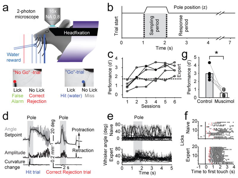
a) A head-fixed mouse under a two-photon microscope. Whisker movements were tracked with high-speed videography. A metal pole was presented either within reach of the whiskers (one of several target locations, blue, ‘Go’-trial) or out-of-reach (red, ‘No Go’-trial).

b) The pole was within reach in the sampling period. Onset of pole movement produced an auditory cue (vertical dotted lines). Answer licks were scored in the answer period.

c) Learning curves. The sensitivity index d′ measures behavioral performance (d′ = 0, chance performance; d′ = 1.75, expert level, gray, approximately 80 % correct trials).

d) Whisker movement and forces. Top, trial showing whisker angle (gray) and setpoint (black). Middle, whisking amplitude (Methods). Bottom, change in whisker curvature, which is proportional to force acting on the follicle. Left, Hit trial; right. Correct Rejection trial.

e) Learning-related changes in whisking. Whisker angle (measured at the base of the whisker, gray) and setpoint (low-pass filtered angle, black) for 20 consecutive Correct Rejection trials in the first (top; d′ = 0.83, first session) fifth session (bottom; d′ = 3.52).

f) Learning-related changes in licking. Licks (ticks; answer licks in red), aligned to first touch, for 20 consecutive Hit trials in naïve (top; d′ = 0.83) and the same animal in the fourth session (bottom; d′ = 3.59).

g) Behavioral performance drops after inactivation of vM1 (n = 5 mice, control, solid circles; muscimol, open circles).

We used videography and automated whisker tracking (Fig. 1a) ²⁷ to determine the mouse’s whisker movements and somatosensory input. Rhythmic whisking (10 – 20 Hz) was superposed on slower changes in setpoint (Fig. 1d, e). Whisking was thus decomposed into setpoint (< 6 Hz) and amplitude (6 – 60 Hz; Methods) ²⁹(Fig. 1d). As a measure of sensory input, we extracted touch-induced changes in whisker curvature, which are proportional to the pressure activating mechanoreceptors in the follicle ^30,31.

Improved performance in the object detection task correlated with changes in motor behavior. Naïve mice whisked occasionally, in a manner unrelated to the trial structure (Fig. 1e), likely reflecting the mouse’s uncertainty about the stimulus-response relationship. In contrast, expert mice protracted their whiskers through a large angle to search for the pole soon (~ 350ms) after it became available (auditory cue, Fig. 1d, e) ²⁷. The repeatability of whisking across trials (ρ=0.57, p<0.001, Pearson’s correlation coefficient, Supplementary Fig. 1a; Methods) and the amplitude of whisker protraction during the sampling period (ρ=0.54, p<0.001, Supplementary Fig. 1b) increased with performance.

Licking consisted of rythmic bouts of 7.2 ± 0.45 Hz ^5,21 (Fig. 1f). The timing of lick bouts with respect to touch became stereotyped with learning. Naïve mice licked with variable latencies (on Hit trials); licking even sometimes preceded touch, indicating that the mice were guessing. Expert mice licked shortly after first touch, and the temporal jitter of the first lick in a bout decreased with performance (ρ = −0.50, p < 0.001, Supplementary Fig. 1c).

Object detection thus relies on a sequence of actions, linked by sensory cues. An auditory cue triggers whisking during the sampling period. Contact between whisker and object causes licking during a response period for a water reward. Silencing vM1 indicates that this task requires the motor cortex. With vM1 silenced, task-dependent whisking persisted, but was reduced in amplitude and repeatability (Supplementary Fig. 1, 2). Task performance dropped, (p<0.001, permutation test, Fig. 1g, Supplementary Fig. 1e). Similar experiments revealed that vS1 is also critical for the object detection task (Supplementary Fig. 1f) ^27,32. These observations imply a critical role for vM1 and vS1 in linking sensation and movement.

Imaging population activity across trials and behavioral sessions

L2/3 cells in vM1 could directly mediate the learned association between whisking, touch and licking. We thus imaged activity of layer 2/3 neurons during learning (Fig. 2). To target vM1 for imaging we injected AAV virus expressing tdTomato ³³ into the C2 column of vS1 and visualized red axonal fluorescence in vM1 (Fig. 2a–d) (Methods). We infected vM1 with the genetically encoded calcium indicator GCaMP3 ³⁴. Long-term expression of GCaMP3 did not cause detectable damage in vivo, nor did it inhibit long-term potentiation in brain slices (Supplementary Fig. 3, 4).

Figure 2. Imaging population activity across trials.

a) Injection sites for GCaMP3 virus in vibrissal motor cortex (vM1) and tdTomato virus in somatosensory cortex (vS1).

b) Glass imaging window (light blue). Bone, light grey; dental cement, dark grey. L2/3 neurons in vM1 receive strong input from vS1 and excite deep layer neurons in vM1.

c–d) GCaMP3 (green) and tdTomato (red) fluorescence image overlaid on a bright-field image (gray). c) Coronal section. d) Imaging window. Box, field of view in e. Bregma, Br.

e) L2/3 neurons expressing GCaMP3 (depth, 210 um). Individual regions (individual neurons) are outlined in purple.

f) Example fluorescence traces (ten neurons, twelve trials). Vertical bars, sampling period (Go trials, blue; No Go trials, red).

g) Example neurons (cell A & B) across one session (329 trials; expert, d′ = 3.13) and simultaneously recorded behaviors. Consecutive Hit, False Alarm, and Correct Rejection trials are arrayed from top to bottom (Misses were rare in this session). Fluorescence intensity was normalized. Curvature changes due to touch occur only during the sampling period in Hit trials, because otherwise the pole was out of reach. Whisking occurred in all trials. Licking occurred in Hit and False Alarm trials. Lower panel: session averages for correct trial types (Hits, blue; Correct Rejections, red).

We imaged GCaMP3-expressing neurons through an imaging window ³⁵ in fields of view overlapping with the red axons (Fig. 2c–e). Images (approximately 250 neurons; Supplementary Table 1), were acquired continuously (4 Hz) over sessions lasting one hour (280 trials; range 141 – 424). Regions of interest were drawn around individual cells to extract fluorescence dynamics caused by neural activity (Fig. 2e; Supplementary Fig. 5). A deconvolution algorithm was used to detect fluorescence events ³⁶, corresponding to small bursts of action potentials (> 2)³⁴ (Supplementary Fig. 5; Methods). Events were detected in 10.6 % of neurons per session (Methods, Supplementary Table 1) (Fig. 2f). 43 % of all neurons showed activity in at least one session. All subsequent analyses were based on these ‘events’ (286 unique neurons; > 10 events per session; 5 animals, 6 sessions per animal). Time series of events were aligned with recordings of behavior, such as whisking, licking, and touch and grouped by trial type (Hit, Correct Rejection, Miss, False Alarm) (Fig. 2g).

Intermingled representations in the motor cortex

L2/3 cells in vM1 receive strong input from vS1. What behaviors are represented by L2/3 cells during active somatosensation? We quantified how well specific behavioral variables could be decoded from neural activity ³⁷. We used Random Forests ³⁸, a generalized form of regression (Methods), to decode behavior based on all neurons (Fig. 3). Each behavioral session was treated separately. The behavioral features measured touch (whisker curvature changes; Fig. 1d) and movements (whisking setpoint, whisking amplitude, licking; Methods; Fig. 1d, f). The algorithm used the activity of populations of neurons to fit individual behavioral features, taking into account dynamics within and across trials (Fig. 3). The explained variance (R_i², for the ith behavioral feature) was used to measure the quality of decoding.

Figure 3. Population decoding of behavioral features.

a–d) Time series of behavioral features (black; down-sampled to the imaging rate, 4 Hz) and a model based on the activity of all active neurons in one session (magenta) (same session as in Fig. 2g). Vertical bars, sampling period (Go trials, blue; No Go trials, red). a) Whisker curvature change. b) Whisking amplitude. c) Whisking setpoint. d) Lick rate. Shuffling trial labels dropped the quality of the fit for all behavioral features (R_i² > R_{i, shuffled}², p < 0.001 for all sessions and animals except for three sessions in which coding of touch was weak; whisking amplitude, mean z-score, 73; whisking setpoint, mean z-score, 28; licking, mean z-score, 23; touch, mean z-score, 10; 1000 shuffles; see Supplementary Fig. 14l,m for an explanation of z-scores).

e) Overlay of whisking at full bandwidth (black) and the model (thick magenta line, whisking setpoint; magenta band, whisking setpoint ± whisking amplitude).

Population activity typically accounted for the recorded behavioral features with high fidelity. The model captured the timing of contact between whisker and object (Fig. 3a) (range of R², 0.03–0.55; for individual mice and sessions see Fig. 6a). Coding of touch in the motor cortex ^18,22 is consistent with direct input from vS1 to the imaged neurons ⁸. The model also predicted motor behaviors (Fig. 3b–e) (whisking amplitude, range of R², 0.22–0.60; whisker setpoint, range of R², 0.22–0.66; lick-rate, range of R², 0.13–0.75). Accurate decoding of whisking amplitude, whisking set-point, and lick-rate suggests that vM1 controls these slowly varying parameters, as expected from previous motor mapping ^{5,8,16,18,29,39} and neurophysiological experiments ^5,29,39. The low sampling rate of imaging may have missed rapid modulation in neural activity ²⁹.

Figure 6. Stability in population decoding.

a) Decoding of behavioral features as a function of behavioral performance. Individual animals correspond to different symbols; lines are linear fits. Top, whisker curvature; middle, whisking setpoint; bottom, lick rate. Whisking amplitude was similar to whisking setpoint and is not shown.

b) Matrix of correlation coefficients for all mice, binned and averaged by behavioral performance (d′). Each point corresponds to a model derived at one value of d′ applied to a session with another value of d′. The points corresponding to models and data from the same session (diagonal) were excluded.

c) Stability of population decoding (representation) of behavioral features (change in R²) as a function of change in behavioral performance. Points derived as in b. Changes in the representation of licking were more predictive with respect to changes in behavioral performance than whisking or touch: Licking, R² = 0.39, F_1,148 = 94; p < 10⁻¹⁷; whisking setpoint, R² = 0.21; F_1,148 = 40; p < 10⁻¹⁷; touch R² = 0.07; F_1,148 = 11; p < 0.001; licking vs setpoint: p < 0.001; Ansari-Bradley test.

We also quantified decoding as a function of the number of neurons (Supplementary Fig. 6). Each behavioral feature required only a tiny number (1.5 – 5.5) to reach saturating decoding. This suggests that the representations underlying object localization are redundant.

How do individual neurons contribute to the population representation? Correlations between activity of individual neurons and specific behaviors were apparent in the raw traces. For example, some neurons were active coincident with whisking during the sampling period, independent of trial type (Cell A, Fig. 2g), while other neurons were active only during licking (Cell B, Fig. 2g) or during other phases of the task (Supplementary Fig. 7–13).

To quantify neuronal representations we again used Random Forests, but here we fit behavioral features using single neurons. The explained variance (R_i², for the ith behavioral feature) was used to measure the quality of decoding by single neurons. Almost one half of the active neurons (42 %) decoded one or more of the measured behavioral features (mean R_i² for best feature, 0.22) (Supplementary Fig. 7), with varying degrees of reliability (Supplementary Fig. 14a–k). Shuffling trial labels dropped the quality of the fit (R_i² > R_{i, shuffled}², p < 0.05 for 351/358 neurons; 1000 shuffles; average z-score, 31; Supplementary Fig. 14l,m), indicating that the Random Forest algorithm captured the covariance of activity and behavior within trials as well as across trials.

We classified neurons into categories (‘touch’, ‘whisking’, ‘licking’), mainly based on the largest correlation coefficient (maximum R_i²) (Supplementary Fig. 7). However, one of the trial types was sometimes more informative than for other trial types and caused the largest overall correlation coefficient to be overruled (Methods) (Supplementary Fig. 7–13). For example, the relationship between neuronal activity and whisking was only evaluated in trials without touch and licking (Correct Rejections). In addition, we considered correlations between activity and sensory variables (object location or forces acting on the whisker, Supplementary Fig. 10, 13, 15). For example, in Hit trials some licking neurons showed activity levels that varied with object location, a signature of sensory input (Supplementary Fig. 8, 11, 13, 15). Such neurons, which correlated with multiple behavioral features, were classified as ‘mixed’ neurons (see Supplementary Fig. 7 and Methods for a full explanation of the classification rules).

The other active neurons remained unclassified based on the measured behavioral features (mean R_i² for best feature, 0.03). However, these neurons still showed interpretable task-related activity (Supplementary Fig. 7). Some neurons became active during errors and others while withholding licking ⁵. Together the unclassified neurons might play roles in cognitive processes; alternatively, they might relate to motor or sensory variables that were not tracked in our study. Overall, only a small fraction of active vM1 neurons expressed any one representation (3 % touch, 26 % whisking, 9 % licking, 4 % mixed), suggesting sparse coding of multiple behavioral features in vM1.

Dynamics of representations with learning

How do individual neurons change with learning? We used the classification of individual neurons to track changes in representations over learning (6 sessions, corresponding to 6–14 days; Methods, Supplementary Fig. 5). Single neurons were dynamic (Fig. 4, Supplementary Fig. 16): cells that decoded a given feature during one session often did not contribute during other sessions, and vice versa. However, when a neuron was classified in different sessions it decoded similar behavioral features (Supplementary Table 2) so that most neurons were classified as part of at most one representation throughout learning (Fig. 4a, c). In particular, whisking neurons rarely became licking neurons and vice versa.

Figure 4. Single neuron representations across learning.

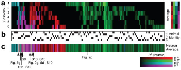
a) Dynamics of classified neurons over learning (cyan, touch; magenta, mixed; red, licking; green, whisking). The intensity of the color indicates the correlation (R²) between data and the model (Methods). Session 1, naïve mice; session 6, expert mice.

b) Animal identity. Each vertical column corresponds to one animal. Black ticks indicate the animal corresponding to the classified cell.

c) Classification of individual neurons averaged across sessions. Arrow heads, neurons with object location-dependent activity. Tagged neurons, data shown in other figures.

All response categories were detected in all animals (Fig. 4a, b; Supplementary Fig. 7) and the representations were spatially intermingled (Supplementary Fig. 16); nearby neurons were equally likely to be part of any of the representations (spatial clustering index, SCI ~ 1.0). These data suggest that motor cortex contains intermingled representations of different movements, and that individual neurons are primed to participate in controlling specific movements.

Learning also altered the timing of neuronal activity. In naïve mice activity was distributed uniformly across the trial (Fig. 5a). With learning, activity of the classified neurons (but not the unclassified neurons) shifted towards the sampling period (Fig. 5b,c; Supplementary Fig. 17). The fraction of neurons that were most active in the sampling period increased by a factor of three, with little change in overall activity levels (Supplementary Fig. 17). These shifts in activity were explained in part by changes in whisking, which became more concentrated in the sampling period with learning (Fig. 1e), and a shorter touch-lick latency (Supplementary Fig. 1). With learning, licking neurons became active earlier within the trial and also began to fire earlier with respect to licking. In naïve mice activity in licking neurons trailed licking (Fig. 5d–f); in expert mice activity anticipated licking (taking the slow kinetics of GCaMP3 fluorescence into account ³⁴). Licking neurons always lagged first touch (Fig. 5e), as did touch neurons (Fig. 5g, h). These learning-related changes in temporal relationships between activity and motor behavior suggest roles of these neurons in controlling movement. Furthermore, nearby neurons can participate in highly specific forms of circuit plasticity during learning.

Figure 5. Plasticity in task-related neuronal dynamics.

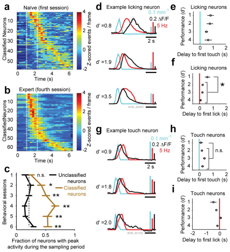
a–b) Trial averages of all classified neurons, ordered by the timing of their peak activity. a) Naïve mice (first session). b) Highly performing mice (fourth session).

c) Fraction of neurons with peak activity during the sampling period of classified (brown) and unclassified neurons (black) as a function of learning (mean ± sem, n = 5 mice). The gray dotted line indicates the expected fraction of neurons if the timing of peak activity was uniformly distributed across the trial (* P<0.05; ** P<0.005; χ² test for each session).

d–i) Temporal parameters of licking and touch neurons, as a function of task performance. Performance (d′) was binned as follows: 1: <1.75, 2: 1.75–2.5, 3: 2.5–3.5, 4: >3.5.

d) PSTHs of touch (change in whisker curvature, cyan), lick rate (red) and fluorescent traces of a representative licking neuron (black) in a naïve (top trace), during learning (middle trace) and an expert animal (bottom trace).

e) Delay from first contact to activity onset in licking neurons (12 neurons, decoding licking for at least 4 days; mean ± sem).

f) Delay from first lick to activity onset in licking neurons. The delay shortened after learning (* P<0.005, Wilcoxon rank sum test).

g) PSTHs of touch (whisker curvature change, cyan), lick rate (red) and calcium transients (black) of a representative touch neuron in a naïve (top trace), during learning (middle trace) and an expert animal (bottom trace).

h) Delay from first contact to activity onset in touch neurons (12 neurons, from 4 animals)

i) Delay from first lick to activity onset in touch neurons.

We next analyzed the dynamics of population-level representations during learning (Fig. 6a–c). We decoded the behavioral features over all experimental sessions and evaluated the quality of the fit as a function of behavioral performance (Fig. 6a). Overall, the representation of licking strengthened, while the number of licks per trial remained stable during learning (Supplementary Fig. 17e). In contrast, the representation of whisking remained stable, even though whisking during the sampling period became more vigorous and purposeful (Fig. 1e, Supplementary Fig. 1).

We assessed the stability of population representations by using the model derived in one session to predict the behavioral features of another session (Fig. 6b). For the first two or three sessions the models derived on one day failed to predict movements on subsequent days, implying labile population representations. However, as the behavior reached a plateau level the representations stabilized, especially for whisking and licking. More than 44 % of the variance in the change in behavioral performance between any two sessions could be explained based on changes in the representations of the different behavioral features (multiple linear regression; p < 10⁻¹⁷; F_4,145 = 29). Changes in the representation of licking were more predictive of the behavioral performance changes than whisking or touch (Fig. 6c). The dynamics of the different representations suggests that vM1 innately controls whisking, but participates in the control of licking only in the context of specific sensorimotor contingencies, such as licking triggered by touch.

Discussion

The precise roles of motor cortex in shaping movement and motor learning have been debated for more than a century (reviewed in ^1,40). Classic recordings from identified PT-type neurons, which carry cortical output to motor centers, revealed activity related to muscle forces and movements ⁴¹. However, PT-type neurons constitute only a tiny fraction of motor cortex neurons ⁷. Simultaneous recordings from diverse neuron types indicate that neuronal ensembles define trajectories of multi-joint movements ^26,42. Conversely, stimulating groups of motor cortex neurons on behavioral time scales evokes complex, ethologically relevant movements ⁴³. vM1 projects to brainstem nuclei controlling facial motor programs including whisking ^19,20 and licking ⁵. Our imaging experiments in vM1 show spatially intermingled representations of various facial movements (Supplementary Fig. 16), all of which are related to performing the object detection task (Fig. 1, 3). These observations together suggest that small regions of motor cortex help to orchestrate goal-directed movements involving multiple body parts.

Motor cortex activity changes with learning ^3–5. Goal-directed movements might thus be established or fine-tuned in the motor cortex. Consistent with this view, representations in L2/3 of motor cortex changed during learning of the object detection task. However, individual L2/3 neurons appear pre-wired to represent particular motor variables: whisking neurons rarely became licking neurons and vice versa (Fig. 4). In expert animals population-level representations were stable (Fig. 6), even with unstable representations of single neurons (Fig. 4, Supplementary Fig. 16). Theoretical work has shown that drifting representations at the level of individual neurons may be critical for motor learning ⁴.

The representation of whisking was strong in L2/3 neurons of naïve animals and remained strong throughout learning (Fig. 6). In contrast, the representation of licking increased with improvements in behavioral performance. Control of voluntary whisking might thus be innate to vM1, whereas vM1 assumes control of licking as the animal learns to initiate licking in response to a specific sensory stimulus (touch, Fig. 1; olfaction ⁵). Enabling flexible associations between sensation and action could be a core function of the superficial layers of the motor cortex.

What could be the cellular mechanisms driving changes in vM1 activity? Learning the object-location task requires chaining a set of sensory-modulated actions into a specific order. Behaviorally, we observed that stereotypic whisking and latency between touch and licking were highly correlated with task proficiency (Fig. 1). Early during learning, activity of L2/3 neurons was distributed uniformly across time, which might provide a basis function ^2,44 to allow appropriate sequences of movements depending on task demands (Fig. 5; Supplementary Fig. 17). After learning, neurons fired mostly during the sampling period, coincident with whisking, touch and onset of licking. This change of timing suggests a role for a dopaminergic reward prediction error signal ⁴⁵, likely arising in the VTA ⁶, which could implement temporal credit assignment in synaptic plasticity ².

METHODS

Chronic window preparation

All procedures were approved by the Janelia Farm Research Campus Institutional Animal Care and Use Committee. We used adult (> P60) male PV-IRES-cre mice (B6;129P2-Pvalbtm1(cre)Arbr/J, The Jackson Laboratory). All surgeries were conducted under isoflurane anesthesia (1.5–2%). Additional drugs reduced potential inflammation (Ketofen, 5mg/kg, subcutaneously) and provided local (Marcaine, 0.5% solution injected under the scalp) and general analgesia (Buprenorphine, 0.1 mg/kg, intraperitoneal). A circular piece of scalp was removed and the underlying bone was cleaned and dried. The periostium was removed with a dental drill and the exposed skull was covered with a thin layer of cyano-acrylic primer (Crazy glue). A custom-machined titanium frame was cemented to the skull with dental acrylic (Lang Dental).

Afferents from the somatosensory cortex were labeled with virus expressing tdTomato ³³ (rAAV-CAG-tdTomato, serotype 2/1; 20 nl at 300 and 550 um depths). The C2 barrel was targeted based on intrinsic signal imaging ²⁸. The virus was injected with a custom, piston-based, volumetric injection system (based on a Narishige, MO-10, manipulator) ⁴⁶. Glass pipettes (Drummond) were pulled and beveled to a sharp tip (30 um outer diameter). Pipettes were back-filled with mineral oil and front-loaded with viral suspension immediately prior to injection.

A craniotomy was made over vM1 (size, 3×2mm; center relative to Bregma: lateral, 0.8 mm; anterior, 1 mm, left hemisphere, Fig. 2a–d). These coordinates were previously determined using intracortical microstimulation ^8,16,18, mapping axonal projections from vS1 in vM1 ^8,47, and trans-cellular labeling with pseudorabies virus (data not shown). Neurons underlying the craniotomy were labeled by injecting virus expressing GCamP3 (rAAV-syn-GCaMP3, serotype 2/1, produced by the University of Pennsylvania Gene Therapy Program Vector Core). The brain was covered with agar (2%). 4–8 sites (10–15 nl/site; depth, 150–210 um; rate, 10 nl/minute) were injected per craniotomy.

The imaging window was constructed from two layers of standard microscope coverglass (Fisher; # 2, thickness, 170 – 210 um), joined with a UV curable optical glue (NOR-61, Norland): a larger piece was attached to the bone; a smaller insert fit snugly into the craniotomy (Fig. 2b, d). The bone surrounding the craniotomy was thinned to allow for a flush fit between insert and the underlying dura.

After virus injection, the glass window was lowered into the craniotomy. The space between the glass and the bone was sealed off with a thin layer of agar (2%), and the window was cemented in place using dental acrylic (Lang Dental). At the end of the surgery, all whiskers on the right side of the snout except row C were trimmed. The mice recovered for 3 days before starting water restriction. Imaging sessions started 14–21 days after the surgery.

Behavior

We designed an object detection task, with three goals in mind: First, animals should be able to learn the task quickly, in a few days. Second, the sensory (whisker contacts and forces) and motor (whisking, licking) behaviors needed to be tracked at high spatial and temporal resolutions throughout learning. Third, we wanted to detect neurons in the motor cortex whose activity patterns might be shaped by sensory input. Since different object locations produce different somatosensory stimuli we presented the object in multiple locations. Neural activity levels that depend on object location then indicate coding of sensory variables.

Behavioral training began after the mice had restricted access to water for at least 7 days (1 ml/day) ^5,28. The behavioral apparatus was designed to fit under a custom built two-photon microscope (https://openwiki.janelia.org/wiki/display/shareddesigns/

Shared+Two-photon+Microscope+Designs). All behavioral training was performed under the microscope while imaging neural activity. In a pre-training session mice learned to lick for water rewards from a lickport (~ 100 rewards). At the same time the brain was inspected for suitable imaging areas. Fields of view were restricted to zones where expression of GCaMP3 and tdTomato (axons from vS1) overlapped (Fig. 2a–d). To escape the vasculature near the midline, imaging was typically performed towards the lateral edge of vM1. Mice with excessive brain movement, limited virus infection or impaired optical access (bone growth, large blood vessels in the vS1 axon projection zone) were excluded from the study.

During the first behavioral session (session 1) the pole was positioned within the range of the whiskers’ resting position, thereby increasing the chance of a whisker-pole collision. As soon as performance reached d′ > 1 the pole was advanced to a more anterior position (~0.5 mm from whisker resting position), forcing the mouse to sample actively for the pole. The target position was adjusted for every session. In expert mice, multiple target positions, all within reach of the whiskers, were introduced to study the effects of object location (Supplementary Fig. 8–11, 13, 15, Supplementary Table 1).

Reversible inactivation

To inactivate vM1 the GABA agonist muscimol was injected into the imaging area in expert mice. A small hole was drilled through the imaging window to allow access for a glass injection pipette. Muscimol hydrobromide (Sigma-Aldrich) was dissolved in saline (5ug/ul) and 50 nl were injected slowly (10nl/min) at depths of 500 and 900 micrometers under the pia ²⁷. The animals were left to recover for two hours before the behavioral session. Inactivation caused a complete absence of fluorescence transients in the imaged field of view (data not shown). Similar methods were used to inactivate vS1 (Supplementary Fig. 1) ²⁷.

Imaging

GCaMP3 was excited using a Ti-Sapphire laser (Chameleon, Coherent) tuned to λ= 1000 nm. We used GaAsP photomultiplier tubes (10770PB-40, Hamamatsu) and a 16x, 0.8 NA microscope objective (Nikon). The field of view was 450×450 um (512×256 pixels; pixel size 0.88 × 1.76 um), imaged at 4 Hz. The microscope was controlled with ScanImage ⁴⁸ (www.scanimage.org). The average power for imaging was < 70 mW, measured at the entrance pupil of the objective. For each mouse the optical axis was adjusted to be perpendicular to the imaging window. Imaging was continuous over behavioral sessions lasting approximately one hour (average, 53 minutes; range, 24 – 72 minutes). Bleaching of GCaMP3 was negligible. Slow drifts of the field of view were corrected manually approximately every 50 trials using a reference image.

Image analysis

To correct for brain motion we used a line-by-line correction algorithm (similar to ⁴⁹, but based on a correlation-based error metric). First, we computed the average of the 5 consecutive frames (chosen from the approximately 40 images comprising a behavioral trial) showing the smallest luminance changes. Each line of each frame was then fit to this reference image using a piecewise rigid gradient descent method.

To align all trials within one session, the average of the trial showing the smallest luminance changes was used as the session reference and all other trials were aligned using normalized cross correlation-based translation.

To extract fluorescence signals from individual cells, regions of interest (ROIs) were drawn based on neuronal shape (individual neurons appeared as fluorescent rings; Supplementary Fig. 5). Mean, maximum intensity, and standard deviation values of all frames of a session were used to determine the boundaries of the neurons. An automated method was used to align the ROIs across sessions. For each ROI, a small square (50 × 50 pixels) around the ROI was selected. Displacements across sessions were calculated by computing the point at which the normalized cross-correlation for this square and the average image of the day peaked. For each ROI, its displacement vector was compared to that of its 5 nearest neighbors. In cases where the displacement exceeded 7 times the median of the neighbors’ displacements, it was set to the median and flagged for manual inspection. The displacements of all ROIs defined a warp field for the entire image.

The pixels in each ROI were averaged to estimate the fluorescence of a single cell. The cell’s baseline fluorescence, F_o, was determined in an iterative manner. First, we estimated the probability distribution function (PDF) of raw fluorescence for each ROI and centered it at its peak (i.e., the peak was assigned a value of 0). A “cutoff value” was calculated by choosing the points below the PDF’s peak and determining the value above which 90% of these values lay (which was negative due to our centering procedure). Cells were ‘moderately active’ if at least 1% of their fluorescence was above twice the absolute value of this “cutoff value” (i.e., the PDF had a long positive tail). Cells were ‘highly active’ if the density at this cutoff value relative peak density exceeded 0.1 (i.e, the PDF’s positive tail was not only long but also fat). All other cells were ‘sparsely active’. The initial F_o estimate was generated by taking a 60 second sliding window over raw fluorescence and using the 50^th, 20^th, or 5^th percentile as F_o for sparsely, moderately, and highly active cells, respectively. Using this first F_o estimate, we computed a preliminary ΔF/F (defined as (F– F_o)/ F_o) and extracted events based on a threshold (3 times the median absolute deviation, MAD). An event period was defined as starting 2 s prior to the peak during a cross of threshold and ending 5s after the peak. In the subsequent F_o estimation procedure, F_o was only estimated for periods without events, and determined via linear interpolation for periods during events. The final ΔF/F trace used for all subsequent analysis was computed using this F_o trace. To produce an event vector from the ΔF/F trace, and thereby minimize the temporal distortions caused by GCaMP3 dynamics ³⁴, we used a non-negative deconvolution method (Supplementary Fig. 5) ³⁶.

Calcium imaging with genetically encoded indicators was crucial for tracking the same neurons across multiple sessions. Furthermore, imaging samples neural activity densely within a region. However, current calcium indicators, including GCamP3, are not sufficiently sensitive to detect single action potentials in vivo and, as a consequence, activity in neurons with very low firing rates was likely missed ^28,34. Our analysis therefore focuses on relatively active neurons. In addition, the slow dynamics (on the order of 100 ms) of the calcium indicator limits the conclusions that can be drawn about connectivity and causality from imaging data.

Approximately 80 % of cortical neurons are pyramidal ⁵⁰. GABAergic interneurons produce much smaller activity-dependent fluorescence changes than pyramidal neurons, presumably because of their short action potentials and high concentrations of endogenous calcium buffer ⁵¹, and their activity were likely not be detected using GCaMP3 ²⁸. For these reasons the vast majority of active neurons detected with our methods were likely excitatory pyramidal neurons.

Long-term expression of GCaMP3

AAV-mediated expression of GCaMP3 provides the high expression levels necessary for in vivo cellular imaging. However, expression continues to increase over months, which can lead to compromised cell health ^34,52, which correlates with break-down of nuclear exclusion. Over the time-course of our experiments (up to 4 weeks of expression) at most 2 % of the cells in the imaged field of view showed nuclear GCaMP3. These neurons were excluded from analysis. In addition, overall event rates were stable across time (Supplementary Fig. 17).

Several observations indicate that imaging did not damage the brain. First, because of the brightness and photostability of GCaMP3 we were able to use low average power. Second, there was no evidence for tissue damage (Supplementary Fig. 3). Third, task-related activity increased with learning in a specific manner, so that some representations (e.g. licking) increased, while other representations did not change (whisking) (Fig. 6). These learning-related changes are inconsistent with non-specific rundown.

Changes in intracellular calcium are necessary to trigger a variety of forms of cellular plasticity. Could GCaMP3 expression interfere with synaptic plasticity? The strength of calcium buffering (‘buffer capacity’) can be estimated as buffer concentration divided by its K_d ⁵³. High concentrations (> 200 uM) of strong (dissociation constant, K_d, 170 nM) calcium buffer (e.g. BAPTA) are required to block synaptic plasticity ^54,55. We estimated the concentration of GCaMP3 (K_d, 660 nM) ³⁴ under our experimental conditions. We harvested acute brain slices from mice that had been used in long-term imaging experiments. We then compared cellular fluorescence at saturating calcium levels, induced by high external K⁺ (20–30 mM) to calibrated GCaMP3 solutions (in standard K+-based internal solution normally used for whole cell recording). Four weeks of expression in L2/3 pyramidal neurons of the visual cortex yielded 76 uM of GCaMP3 ⁵². 7 weeks of expression in vM1 gave 130 uM of GCaMP. These experiments imply that GCaMP3 produces lower buffer capacity than BAPTA concentrations that are known not to perturb synaptic plasticity (buffer capacities, < 200 vs > 1200). Consistently, expression of GCaMP3 did not perturb induction of long-term potentiation in hippocampal brain slices (Supplementary Fig. 4) (GCaMP3 concentration, 15 uM, determined as above).

We further tested whether GCaMP3 expression level influenced the plasticity of neuronal responses. Relative baseline fluorescence measured in individual neurons was constant across days and thus was a good indicator of GCaMP3 expression. We calculated the probability that a classified cell remained active and retained its classification (i.e. was stable). We compared stability in the 25% brightest and dimmest neurons. Dim and bright cells were similarly stable (dim cells, 65% stable; bright cells, 60 % stable; χ²=0.39; P>0.5). This analysis suggests that under our conditions GCaMP3 does not obviously perturb cellular plasticity in vivo.

Other measurements also imply that plasticity was not obviously impaired by long-term expression of GCaMP3. Circuit function is shaped by ongoing plasticity, integrated over the recent past. Neurons with long-term expression of GCaMP3 generally show normal circuit properties. Orientation and direction selectivity are normal in GCaMP3-expressing L2/3 neurons in mouse V1 ⁵² and hippocampal place cells are normal in CA1 neurons in the hippocampus ⁵⁶. The sparseness and response types of L2/3 neurons in vS1 are indistinguishable when measured with electrophysiological methods or GCaMP3 ²⁸. Finally, in our experiments L2/3 neurons showed specific learning-related changes in activity in vivo (Fig. 4–6).

Whisker tracking

Whiskers were illuminated with a high power LED (940 nm, Roithner) and condenser optics (Thorlabs). Images were acquired through a telecentric lens (0.36X, Edmund Optics) by a high-speed CMOS camera (EoSense CL, Mikrotron, Germany) running at 500 frames/sec (640 × 352 pixels; resolution, 42 pixels/mm). Image acquisition was controlled by Streampix 3 (Norpix, Canada). The whisker position and shape were tracked using automated procedures ²⁷. Whiskers are cantilevered beams, with one end embedded in the follicle in the whisker pad. The mechanical forces acting on the follicles can be extracted from the shape changes after contact between whisker and object. For example, a change in curvature at point p along the whisker is proportional to the force applied by the pole on the whisker ³⁰: F ~ Δκ_p y_p, where y_p is the bending stiffness at p (approximately 3 mm from the follicle). We thus present forces on the whiskers as the change in curvature, Δκ These forces underlie object localization ^27,31. Δκ was determined using a parametric curve comprising 2^nd order polynomial fits to the whisker backbone. Periods of contact between whisker and object (touch) were detected based on nearest distance between whisker and object and Δκ. A total of ~13,000,000 whisker video images, comprising ~7500 behavioral trials, were analyzed for this project.

Expert mice contacted the pole multiple times with one or several whiskers (average number of contacts for the dominant whisker, 8; range 0–19) before their decision (signaled by an answer lick on correct Go trials).

Behavioral features

We analyzed neural activity with respect to multiple behavioral features. Licks were detected with a lickometer ²⁷ and lick rate (Hz) was defined as the inverse of the inter-lick interval. Our imaging rate (4 Hz) was slower than the rapid components of rhythmic whisking (10–20 Hz). In addition, motor cortex neurons primarily code for the slowly varying whisking variables, setpoint and amplitude ^29,39. Whisker setpoint was the low pass filtered (6 Hz) whisker angle. Whisker amplitude was defined as the Hilbert transform ²⁹ of the absolute value of the band-pass filtered (6–60 Hz) whisker angle (Fig. 1d). Since whiskers move mostly together ²⁷ setpoint and amplitude were averaged across all whiskers. The time derivatives of whisker setpoint and amplitude were used as independent features. Δκ was measured during the sampling period. Protraction touch (positive curvature changes), retraction touch (negative curvature changes) and absolute values were treated separately. All behavioral features were down-sampled to match the image acquisition rate (4 Hz). Mean and maximum values were calculated for each feature in a 250 ms window centered on the middle of the new sampling point.

Decoding behavioral variables

The relationship between the calcium activity x_i of the ith neuron and the jth behavioral variable y_i can be characterized as an encoding description P(x_i|y_j) or a decoding description P(y_f|x_t). The encoding description specifies how much of neuronal activity can be accounted for by behavioral variables. The decoding description specifies how behavioral variables can be derived from activity of one neuron or neuronal populations. Here, we focused on the decoding description.

We used machine learning algorithms to decode behavioral features based on activity. The input to the algorithm was the event-rate (i.e. deconvoluted ΔF/F). To predict sensory input we also used time-shifted future activity. For motor variables we used both past and future activty, since neural activity could reflect motor commands, corollary discharges, or re-afferent input.

The goal of the decoder algorithm was to find a mapping ŷ_f(t_k) = f[x_t(t_k-l),…,x_t(t_k),…,x_t(t_k+p)] that best approximates y_f(t_k) for all t_k (discretized time in units of 0.25s, corresponding to the imaging rate); l and p represent the maximum negative and positive shifts of the activity respectively.

We concatenated trials to generate a vector t̄ of time-binned data. For sensory variables we used l=2 and p=0 and for sensory-motor variables l=2 and p=2 (corresponding to time-shifts up to 0.5s). The dimensionality of the input variables is l+p+1. To simplify the notation we define the vector x̄_i,n as the activity of cell i at all times shifted n frames to the future. The algorithm was trained on a subset of trials (the training set; 80 %) and evaluated on a separate set of test trials (20%). We repeated this procedure five times to obtain a prediction for all trials ³⁸.

The accuracy of decoding was evaluated using the Pearson correlation coefficient (ρ) between the model estimate and the data. The explained variance is R² = ρ² (range 0 – 1). R² was calculated separately for each trial type (i.e. Hit, Correct Rejection, Miss and False Alarm). Treating trial types separately was critical to disambiguate the relationship between different behavioral variables and activity. For instance, we observed large amplitude whisking during licking, which complicates the classification of neuronal responses. However, during Correct Rejection trials, licking was absent and whisking present, allowing classification. Similarly, in trained animals, touch and licking occurred with short latencies in Hit trials (Fig. 1, 5). In contrast in False Alarm trials touch was absent.

Decoding was done with Random Forests ^38,57, a multivariate, non-parametric machine learning algorithm based on bootstrap aggregation (i.e. bagging) of regression trees. We used the TreeBagger class implemented in Matlab®. TreeBagger requires only few parameters: the number of trees (N_trees = 126), the minimum leaf size (minleaf = 5), the number of features chosen randomly at each split (N_spilt –N_features/3; the typical value used by default). These parameters were chosen as a trade-off between decoder accuracy and computation time. We did not observe much improvement in decoding accuracy for N_trees > 32 and minleaf < 10 (data not shown).

Classification of response-types

We measured the R² between each measured behavioral variable (i.e. whisking speed, lick-rate, whisking setpoint, etc) and each cell’s decoder prediction for all the trials and for each trial type. We considered only cells with more than one event in a session. In addition, for sessions with multiple-pole positions we used an Analysis of Variance (ANOVA) to determine if the contact evoked calcium response was different for the different pole position (Supplementary Fig. 8–11, 13, 15). We grouped the behavioral variables in larger categories such as whisking (i.e. including whisking amplitude, setpoint and speed), lick rate and touch (i.e. touch per whisker, rate of change of forces, absolute magnitude, etc). We considered the best R² set for each of the three behavioral categories. Alternatively, all cells were manually classified based on trial-to-trial calcium transients and behavioral prediction for each trial-type. For most cells (>82%) classification was unambiguous based on the decoder R² values. The remaining cells were more accurately classified based on a rarer trial type (typically False Alarm trials). Three of the authors independently arrived at consistent classifications.

Population decoding

For decoding neural populations (Fig. 3, 6) we considered all neurons showing at least 1 event and created an input vector of size N_neurons × (l+p+1). We trained the Random Forest algorithm to decode each of the behavioral variables and evaluated the quality of the fit as before.

With the model based on data from one day we tested decoding of behavioral variables on another day. To compare data between two different days, we normalized the neural activity and the behavioral variables using a z-score transformation (i.e. by subtracting the mean and dividing by the standard deviation). In addition, some cells were active one day but not on other days. We labeled these neurons as missing data.

Measurement of synaptic plasticity in brain slices

Rat hippocampal slice cultures were prepared at postnatal day 4–5 ⁵⁸. Plasmids encoding GCaMP3 and cerulean were under the control of a human synapsin1 promoter were electroporated into single CA1 pyramidal neurons after 18 days in vitro (1:1 ratio; 50 ng/ul each) (modified from ref. ⁵⁹). Recordings were done 3–7 days after transfection. GCaMP3 was largely excluded from the nucleus and cell morphology was indistinguishable from neurons expressing cerulean alone. Paired whole-cell recordings from CA1 and CA3 pyramidal cells were made at room temperature (21–23 °C), using 3–4 MOhm pipettes containing (in mM): 135 K-gluconate, 4 MgCl₂, 4 Na₂-ATP, 0.4 Na-GTP, 10 Na₂-phosphocreatine, 3 ascorbate, and 10 Hepes (pH 7.2). ACSF consisted of (in mM): 135 NaCl, 2.5 KCl, 4 CaCl₂, 4 MgCl₂, 10 Na-HEPES, 12.5 D-glucose, 1.25 NaH₂PO₄ (pH 7.4). EPSCs were measured at −65 mV holding potential.

References

- 1.Scott SH. Inconvenient truths about neural processing in primary motor cortex. The Journal of physiology. 2008;586:1217–1224. doi: 10.1113/jphysiol.2007.146068. [DOI] [PMC free article] [PubMed] [Google Scholar]
- 2.Wolpert DM, Diedrichsen J, Flanagan JR. Principles of sensorimotor learning. Nature reviews. Neuroscience. 2011;12:739–751. doi: 10.1038/nrn3112. [DOI] [PubMed] [Google Scholar]
- 3.Wise SP, Moody SL, Blomstrom KJ, Mitz AR. Changes in motor cortical activity during visuomotor adaptation. Experimental brain research. Experimentelle Hirnforschung. Experimentation cerebrale. 1998;121:285–299. doi: 10.1007/s002210050462. [DOI] [PubMed] [Google Scholar]
- 4.Rokni U, Richardson AG, Bizzi E, Seung HS. Motor learning with unstable neural representations. Neuron. 2007;54:653–666. doi: 10.1016/j.neuron.2007.04.030. [DOI] [PubMed] [Google Scholar]
- 5.Komiyama T, et al. Learning-related fine-scale specificity imaged in motor cortex circuits of behaving mice. Nature. 2010;464:1182–1186. doi: 10.1038/nature08897. [DOI] [PubMed] [Google Scholar]
- 6.Hosp JA, Pekanovic A, Rioult-Pedotti MS, Luft AR. Dopaminergic projections from midbrain to primary motor cortex mediate motor skill learning. The Journal of neuroscience : the official journal of the Society for Neuroscience. 2011;31:2481–2487. doi: 10.1523/JNEUROSCI.5411-10.2011. [DOI] [PMC free article] [PubMed] [Google Scholar]
- 7.Keller A. Intrinsic synaptic organization of the motor cortex. Cereb Cortex. 1993;3:430–441. doi: 10.1093/cercor/3.5.430. [DOI] [PubMed] [Google Scholar]
- 8.Mao T, et al. Long-Range Neuronal Circuits Underlying the Interaction between Sensory and Motor Cortex. Neuron. 2011;72:111–123. doi: 10.1016/j.neuron.2011.07.029. [DOI] [PMC free article] [PubMed] [Google Scholar]
- 9.Hooks BM, et al. Laminar analysis of excitatory local circuits in vibrissal motor and sensory cortical areas. PLoS Biol. 2011;9:e1000572. doi: 10.1371/journal.pbio.1000572. [DOI] [PMC free article] [PubMed] [Google Scholar]
- 10.Anderson CT, Sheets PL, Kiritani T, Shepherd GM. Sublayer-specific microcircuits of corticospinal and corticostriatal neurons in motor cortex. Nat Neurosci. 2010;13:739–744. doi: 10.1038/nn.2538. [DOI] [PMC free article] [PubMed] [Google Scholar]
- 11.Kaneko T, Cho R, Li Y, Nomura S, Mizuno N. Predominant information transfer from layer III pyramidal neurons to corticospinal neurons. J Comp Neurol. 2000;423:52–65. doi: 10.1002/1096-9861(20000717)423:1<52::AID-CNE5>3.0.CO;2-F. [pii] [DOI] [PubMed] [Google Scholar]
- 12.Kaneko T, Caria MA, Asanuma H. Information processing within the motor cortex. II.Intracortical connections between neurons receiving somatosensory cortical input and motor output neurons of the cortex. J Comp Neurol. 1994;345:172–184. doi: 10.1002/cne.903450203. [DOI] [PubMed] [Google Scholar]
- 13.Pavlides C, Miyashita E, Asanuma H. Projection from the sensory to the motor cortex is important in learning motor skills in the monkey. Journal of neurophysiology. 1993;70:733–741. doi: 10.1152/jn.1993.70.2.733. [DOI] [PubMed] [Google Scholar]
- 14.Iriki A, Pavlides C, Keller A, Asanuma H. Long-term potentiation in the motor cortex. Science. 1989;245:1385–1387. doi: 10.1126/science.2551038. [DOI] [PubMed] [Google Scholar]
- 15.Rioult-Pedotti MS, Friedman D, Hess G, Donoghue JP. Strengthening of horizontal cortical connections following skill learning. Nat Neurosci. 1998;1:230–234. doi: 10.1038/678. [DOI] [PubMed] [Google Scholar]
- 16.Li CX, Waters RS. Organization of the mouse motor cortex studied by retrograde tracing and intracortical microstimulation (ICMS) mapping. Can J Neurol Sci. 1991;18:28–38. doi: 10.1017/s0317167100031267. [DOI] [PubMed] [Google Scholar]
- 17.Brecht M, et al. Organization of rat vibrissa motor cortex and adjacent areas according to cytoarchitectonics, microstimulation, and intracellular stimulation of identified cells. J Comp Neurol. 2004;479:360–373. doi: 10.1002/cne.20306. [DOI] [PubMed] [Google Scholar]
- 18.Ferezou I, et al. Spatiotemporal dynamics of cortical sensorimotor integration in behaving mice. Neuron. 2007;56:907–923. doi: 10.1016/j.neuron.2007.10.007. [DOI] [PubMed] [Google Scholar]
- 19.Hattox AM, Priest CA, Keller A. Functional circuitry involved in the regulation of whisker movements. J Comp Neurol. 2002;442:266–276. doi: 10.1002/cne.10089. [pii] [DOI] [PMC free article] [PubMed] [Google Scholar]
- 20.Grinevich V, Brecht M, Osten P. Monosynaptic pathway from rat vibrissa motor cortex to facial motor neurons revealed by lentivirus-based axonal tracing. J Neurosci. 2005;25:8250–8258. doi: 10.1523/JNEUROSCI.2235-05.2005. [DOI] [PMC free article] [PubMed] [Google Scholar]
- 21.Travers JB, Dinardo LA, Karimnamazi H. Motor and premotor mechanisms of licking. Neurosci Biobehav Rev. 1997;21:631–647. doi: 10.1016/s0149-7634(96)00045-0. S0149-7634(96)00045-0 [pii] [DOI] [PubMed] [Google Scholar]
- 22.Kleinfeld D, Sachdev RN, Merchant LM, Jarvis MR, Ebner FF. Adaptive filtering of vibrissa input in motor cortex of rat. Neuron. 2002;34:1021–1034. doi: 10.1016/s0896-6273(02)00732-8. [DOI] [PubMed] [Google Scholar]
- 23.Sato TR, Svoboda K. The functional properties of barrel cortex neurons projecting to the primary motor cortex. J Neurosci. 2010;30:4256–4260. doi: 10.1523/JNEUROSCI.3774-09.2010. [DOI] [PMC free article] [PubMed] [Google Scholar]
- 24.Ganguly K, Carmena JM. Emergence of a stable cortical map for neuroprosthetic control. PLoS biology. 2009;7:e1000153. doi: 10.1371/journal.pbio.1000153. [DOI] [PMC free article] [PubMed] [Google Scholar]
- 25.Stosiek C, Garaschuk O, Holthoff K, Konnerth A. In vivo two-photon calcium imaging of neuronal networks. Proc Natl Acad Sci U S A. 2003;100:7319–7324. doi: 10.1073/pnas.1232232100. [DOI] [PMC free article] [PubMed] [Google Scholar]
- 26.Dombeck DA, Graziano MS, Tank DW. Functional clustering of neurons in motor cortex determined by cellular resolution imaging in awake behaving mice. J Neurosci. 2009;29:13751–13760. doi: 10.1523/JNEUROSCI.2985-09.2009. [DOI] [PMC free article] [PubMed] [Google Scholar]
- 27.O’Connor DH, et al. Vibrissa-based object localization in head-fixed mice. J Neurosci. 2010;30:1947–1967. doi: 10.1523/JNEUROSCI.3762-09.2010. [DOI] [PMC free article] [PubMed] [Google Scholar]
- 28.O’Connor DH, Peron SP, Huber D, Svoboda K. Neural activity in barrel cortex underlying vibrissa-based object localization in mice. Neuron. 2010;67:1048–1061. doi: 10.1016/j.neuron.2010.08.026. [DOI] [PubMed] [Google Scholar]
- 29.Hill DN, Curtis JC, Moore JD, Kleinfeld D. Primary motor cortex reports efferent control of vibrissa motion on multiple timescales. Neuron. 2011;72:344–356. doi: 10.1016/j.neuron.2011.09.020. [DOI] [PMC free article] [PubMed] [Google Scholar]
- 30.Birdwell JA, et al. Biomechanical models for radial distance determination by the rat vibrissal system. J Neurophysiol. 2007;98:2439–2455. doi: 10.1152/jn.00707.2006. [DOI] [PubMed] [Google Scholar]
- 31.Knutsen PM, Ahissar E. Orthogonal coding of object location. Trends Neurosci. 2008 doi: 10.1016/j.tins.2008.10.002. [DOI] [PubMed] [Google Scholar]
- 32.Hutson KA, Masterton RB. The sensory contribution of a single vibrissa’s cortical barrel. J Neurophysiol. 1986;56:1196–1223. doi: 10.1152/jn.1986.56.4.1196. [DOI] [PubMed] [Google Scholar]
- 33.Shaner NC, et al. Improved monomeric red, orange and yellow fluorescent proteins derived from Discosoma sp. red fluorescent protein. Nat Biotechnol. 2004 doi: 10.1038/nbt1037. [DOI] [PubMed] [Google Scholar]
- 34.Tian L, et al. Imaging neural activity in worms, flies and mice with improved GCaMP calcium indicators. Nat Methods. 2009;6:875–881. doi: 10.1038/nmeth.1398. [DOI] [PMC free article] [PubMed] [Google Scholar]
- 35.Trachtenberg JT, et al. Long-term in vivo imaging of experience-dependent synaptic plasticity in adult cortex. Nature. 2002;420:788–794. doi: 10.1038/nature01273. [DOI] [PubMed] [Google Scholar]
- 36.Vogelstein JT, et al. Fast nonnegative deconvolution for spike train inference from population calcium imaging. Journal of neurophysiology. 2010;104:3691–3704. doi: 10.1152/jn.01073.2009. [DOI] [PMC free article] [PubMed] [Google Scholar]
- 37.Graf AB, Kohn A, Jazayeri M, Movshon JA. Decoding the activity of neuronal populations in macaque primary visual cortex. Nat Neurosci. 14:239–245. doi: 10.1038/nn.2733. [DOI] [PMC free article] [PubMed] [Google Scholar]
- 38.Hastie T, Tibshirani R, Friedman J. The Elements of Statistical Learning. 2. Springer; 2009. [Google Scholar]
- 39.Carvell GE, Miller SA, Simons DJ. The relationship of vibrissal motor cortex unit activity to whisking in the awake rat. Somatosens Mot Res. 1996;13:115–127. doi: 10.3109/08990229609051399. [DOI] [PubMed] [Google Scholar]
- 40.Graziano MSA. The Intelligent Movement Machine. 1. Oxford: 2009. [Google Scholar]
- 41.Evarts EV. Relation of pyramidal tract activity to force exerted during voluntary movement. J Neurophysiol. 1968;31:14–27. doi: 10.1152/jn.1968.31.1.14. [DOI] [PubMed] [Google Scholar]
- 42.Afshar A, et al. Single-trial neural correlates of arm movement preparation. Neuron. 2011;71:555–564. doi: 10.1016/j.neuron.2011.05.047. [DOI] [PMC free article] [PubMed] [Google Scholar]
- 43.Graziano MS, Aflalo TN. Mapping behavioral repertoire onto the cortex. Neuron. 2007;56:239–251. doi: 10.1016/j.neuron.2007.09.013. [DOI] [PubMed] [Google Scholar]
- 44.Salinas E. Rank-order-selective neurons form a temporal basis set for the generation of motor sequences. The Journal of neuroscience : the official journal of the Society for Neuroscience. 2009;29:4369–4380. doi: 10.1523/JNEUROSCI.0164-09.2009. [DOI] [PMC free article] [PubMed] [Google Scholar]
- 45.Schultz W, Dayan P, Montague PR. A neural substrate of prediction and reward. Science. 1997;275:1593–1599. doi: 10.1126/science.275.5306.1593. [DOI] [PubMed] [Google Scholar]
- 46.Petreanu L, Mao T, Sternson SM, Svoboda K. The subcellular organization of neocortical excitatory connections. Nature. 2009;457:1142–1145. doi: 10.1038/nature07709. [DOI] [PMC free article] [PubMed] [Google Scholar]
- 47.Porter LL, White EL. Afferent and efferent pathways of the vibrissal region of primary motor cortex in the mouse. J Comp Neurol. 1983;214:279–289. doi: 10.1002/cne.902140306. [DOI] [PubMed] [Google Scholar]
- 48.Pologruto TA, Sabatini BL, Svoboda K. ScanImage: Flexible software for operating laser-scanning microscopes. BioMedical Engineering OnLine. 2003;2:13. doi: 10.1186/1475-925X-2-13. [DOI] [PMC free article] [PubMed] [Google Scholar]
- 49.Greenberg DS, Kerr JN. Automated correction of fast motion artifacts for two-photon imaging of awake animals. J Neurosci Methods. 2008 doi: 10.1016/j.jneumeth.2008.08.020. [DOI] [PubMed] [Google Scholar]
- 50.Gonchar Y, Wang Q, Burkhalter A. Multiple distinct subtypes of GABAergic neurons in mouse visual cortex identified by triple immunostaining. Front Neuroanat. 2007;1:3. doi: 10.3389/neuro.05.003.2007. [DOI] [PMC free article] [PubMed] [Google Scholar]
- 51.Kerlin AM, Andermann ML, Berezovskii VK, Reid RC. Broadly tuned response properties of diverse inhibitory neuron subtypes in mouse visual cortex. Neuron. 2010;67:858–871. doi: 10.1016/j.neuron.2010.08.002. [DOI] [PMC free article] [PubMed] [Google Scholar]
- 52.Zariwala HA, et al. A cre-dependent GCaMP3 reporter mouse for neuronal imaging in vivo. J Neurosci. 2012 doi: 10.1523/JNEUROSCI.4469-11.2012. in press. [DOI] [PMC free article] [PubMed] [Google Scholar]
- 53.Maravall M, Mainen ZM, Sabatini BL, Svoboda K. Estimating intracellular calcium concentrations and buffering without wavelength ratioing. Biophys J. 2000;78:2655–2667. doi: 10.1016/S0006-3495(00)76809-3. [DOI] [PMC free article] [PubMed] [Google Scholar]
- 54.Nevian T, Sakmann B. Spine Ca2+ signaling in spike-timing-dependent plasticity. The Journal of neuroscience : the official journal of the Society for Neuroscience. 2006;26:11001–11013. doi: 10.1523/JNEUROSCI.1749-06.2006. [DOI] [PMC free article] [PubMed] [Google Scholar]
- 55.Gordon U, Polsky A, Schiller J. Plasticity compartments in basal dendrites of neocortical pyramidal neurons. J Neurosci. 2006;26:12717–12726. doi: 10.1523/JNEUROSCI.3502-06.2006. [DOI] [PMC free article] [PubMed] [Google Scholar]
- 56.Dombeck DA, Harvey CD, Tian L, Looger LL, Tank DW. Functional imaging of hippocampal place cells at cellular resolution during virtual navigation. Nat Neurosci. 2010;13:1433–1440. doi: 10.1038/nn.2648. [DOI] [PMC free article] [PubMed] [Google Scholar]
- 57.Breiman L. Random forests. Mach Learn. 2001;45:5–32. [Google Scholar]
- 58.Stoppini L, Buchs PA, Muller DA. A simple method for organotypic cultures of nervous tissue. J Neurosci Methods. 1991;37:173–182. doi: 10.1016/0165-0270(91)90128-m. [DOI] [PubMed] [Google Scholar]
- 59.Rathenberg J, Nevian T, Witzemann V. High-efficiency transfection of individual neurons using modified electrophysiology techniques. J Neurosci Methods. 2003;126:91–98. doi: 10.1016/s0165-0270(03)00069-4. [DOI] [PubMed] [Google Scholar]
Associated Data
This section collects any data citations, data availability statements, or supplementary materials included in this article.