Functional divisions for visual processing in the central brain of flying Drosophila

Significance

Neuroanatomical methods are limited in their ability to identify functions of neurons in living brains, and recordings in restrained animals cannot be used to study pathways that are only active during naturalistic behaviors. In this study, we investigated a central brain region thought to be involved in both sensory processing and motor output in insects. To examine its role in the sensory-motor transformation, we imaged neuronal activity in tethered flying flies responding to visual stimuli. While the animals were flying, we observed separate functional subunits defined by their responses to visual stimulation. During quiescence, however, these subunits were inactive and indistinguishable from one another. This context-dependent processing suggests that this brain region is involved in visual navigation during flight.

Abstract

Although anatomy is often the first step in assigning functions to neural structures, it is not always clear whether architecturally distinct regions of the brain correspond to operational units. Whereas neuroarchitecture remains relatively static, functional connectivity may change almost instantaneously according to behavioral context. We imaged panneuronal responses to visual stimuli in a highly conserved central brain region in the fruit fly, Drosophila, during flight. In one substructure, the fan-shaped body, automated analysis revealed three layers that were unresponsive in quiescent flies but became responsive to visual stimuli when the animal was flying. The responses of these regions to a broad suite of visual stimuli suggest that they are involved in the regulation of flight heading. To identify the cell types that underlie these responses, we imaged activity in sets of genetically defined neurons with arborizations in the targeted layers. The responses of this collection during flight also segregated into three sets, confirming the existence of three layers, and they collectively accounted for the panneuronal activity. Our results provide an atlas of flight-gated visual responses in a central brain circuit.

The central complex (CX) is a system of unpaired neuropils in the adult insect brain consisting of the protocerebral bridge (PB), the fan-shaped body (FB), and the ellipsoid body (EB) (Movie S1). The architecture of these neuropils is remarkably conserved across species (1, 2) such that systems of columnar and tangential neurons obey intricate wiring rules (3–5). In addition to the three primary structures, all winged insects possess paired noduli (NO) that are intimately connected to the rest of the CX (2). Despite the stereotyped structure of the CX, there is as yet no consensus regarding its function. In the desert locust Schistocerca gregaria, numerous CX neurons respond to the angle of linearly polarized light (6, 7) and other visual features (8). In the cockroach Blaberus discoidalis, some units in the CX respond to visual motion (9) and mechanosensation (10), whereas others fire during motor actions such as running and turning (11, 12). Studies in fruit flies suggest that the CX is important for locomotion (13), certain types of climbing (14), visual learning and memory (15–17), and various other tasks involved in visual processing (18–21).

To gain a more coherent understanding of CX function, we sought an unbiased approach to investigate its role systematically in different behavioral contexts and in a variety of stimulus conditions. We designed a broad panel of visual stimuli that are known to be important for guidance and stability during flight. Recent advances in the sensitivity of genetically encoded calcium indicators made it possible to record panneuronal responses to these stimuli during tethered flight using multiphoton imaging. Although all three primary neuropils of the CX contained neurons that responded to the stimuli, only in the FB did we observe responses during flight that were absent when the animals were not flying. We identified three functional layers in the FB with distinct patterns of flight-dependent visual responses. The responses of the ventral two layers are consistent with this structure playing a role in controlling heading in the horizontal plane during flight. By screening a web-based dataset of over 6,000 annotated expression patterns, we assembled a collection of driver lines sufficiently large to include most, if not all, of the FB neurons. Our results provide an unbiased analysis of cell types involved in generating flight-dependent visual responses in the CX.

Results

All Regions of the CX Respond to Visual Stimuli.

To map responses in the CX, we designed a diverse panel of 18 visual stimuli known to elicit locomotor responses in walking and flying flies (Movie S2). The panel included looming or drifting objects, large-field patterns of optic flow, and a rotating field of polarized UV light. The stimuli can be divided into two categories: six pairs of midline-asymmetrical stimuli in which one stimulus is the mirror image of its partner (Fig. 1A) and six stimuli that are each symmetrical about the animal’s midline (Fig. 1C). We presented these stimuli in random order while each animal was flying and when it was quiescent, and imaged neuronal activity in the CX. During flight bouts, we simultaneously measured the stroke amplitude of the two wings. In free flight, changes in stroke amplitude contribute to changes in roll, pitch, and yaw moments (22) that alter flight course. In tethered flies, stroke amplitude serves as a proxy for intended turns. To ensure that our analysis would be functionally relevant, we verified that all of the stimuli were sufficiently salient to elicit changes in wing motion reliably, although the responses to the rotating polarizer were small. For stimuli that were asymmetrical with respect to the midline (e.g., a vertical stripe moving rightward), we first decomposed each trial into responses of the right and left wings (Fig. 1B). We then grouped each set of responses of a single wing with the contralateral wing responses to the mirror image stimulus (e.g., we grouped the right wing responses to a stripe moving rightward, with the left wing responses to a stripe moving leftward; Fig. 1E). For stimuli that were symmetrical about the midline (e.g., a horizontal stripe moving upward), no such decomposition is necessary (Fig. 1D), and the responses of both wings are plotted together (Fig. 1F).

Fig. 1.

(A and C) Schematic representations of visual stimuli. Polarizer stimuli are schematic of direction only. All other stimuli are represented by a weighted average of the first third of the stimulus, with the weighted intensity of each pixel decreasing back in time. (A, B, and E) Midline-asymmetrical stimulus pairs. (B) Explanation of our plotting convention for midline-asymmetrical stimulus pairs. Single wing responses are grouped with the other wing responses to the mirror-reflected stimulus. (C, D, and F) Midline-symmetrical stimuli and plotting convention. (D) For midline-symmetrical stimuli, no decomposition is necessary. (E and F) Mean of wing responses of all flies used in our study to all stimuli (red for left wings, blue for right wings, and black for both wings). Ipsi., ipsilateral.

First, to provide a coarse map of the visual responses of the CX during flight, we used the GAL4/UAS binary expression system to drive expression of GCaMP6f (23) and tdTomato (24) in all neurons with R57C10-GAL4 (25). We corrected for brain motion by using the tdTomato signal to register each frame to a reference image acquired at the start of the experiment. In addition, we normalized the GCaMP6f signal to the tdTomato signal to reduce the effect of correlated changes in both signals caused by vertical brain motion. To examine neuronal responses, we used the same convention described above for wing stroke amplitude: For stimuli that were asymmetrical about the midline, we decomposed each trial into the responses of the ipsilateral and contralateral brain hemispheres (Fig. 2 D–G).

Fig. 2.

Panneuronal responses during flight and quiescence in four CX neuropils. (A–C) Anatomy of the CX. Optical sections from a composite of warped confocal image stacks of seven GAL4 lines used in our study (also Movie S1) are shown. Each line is shown in a different color in the composite images (red, R94C05; green, R42B05; blue, R73D06; gray, R52G12; cyan, R38E07; magenta, R44B10; and yellow, R95F02). (Scale bar: 50 μm.) (A) Frontal section through the PB. (B) Frontal section through the FB and NO. (C) Frontal section through the EB and bulbs (BU). (Far Left; green bounding box) Sagittal section at the position indicated by green lines in frontal sections; rostral is right. (Lower; cyan bounding box) Horizontal section at height indicated by cyan lines; rostral is up. (D–G) Time series data for the ratio, R, of GCaMP6f fluorescence to tdTomato fluorescence in each hemisphere. The baseline for the calculation of ΔR/R is the mean R during the 1 s before all stimulus onset during quiescence. The plotting convention is the same as in Fig. 1 (e.g., in the first column of G, the response of the left BU to a looming feature presented on the left and the response of the right BU to a looming feature presented on the right are averaged together). Black lines indicate trials during which the animal was flying, and gray lines indicate the animal was not flying. Patches indicate 95% confidence intervals, and yellow indicates departures from prestimulus baseline at the P < 0.05 level based on the Mann–Whitney U test with Bonferroni correction for 144 comparisons (18 trial types × 2 flight conditions × 4 neuropil regions). (D) PB, n = 7 animals. (E) FB, n = 9 animals. (F) NO, n = 7 animals. (G) BU, an input region to the EB, n = 5 animals. (D–G, Right) Images are mean GCaMP6f signal from the entire experiment of a representative individual animal in gray with overlaid regions of interest of the left and right hemispheres in red and blue, respectively. (Scale bars: 20 μm.)

Neurons in the PB responded to a vertical stripe moving from the contralateral side to the ipsilateral side when the animal was not flying (Fig. 2D, gray trace). We also observed responses to a vertical stripe moving in the opposite direction and a large-field stimulus moving horizontally. During flight, the baseline PB fluorescence increased in the absence of any visual stimulus, but the stimulus-elicited fluorescence changes were modest relative to this elevated baseline (Fig. 2D, black trace). Automated clustering of the functional responses (details are provided in Materials and Methods) revealed translational symmetry, as opposed to bilateral symmetry, between the two hemispheres (Fig. S1), consistent with previous studies of the anatomical connectivity in the PB (4, 5). In the FB and closely related NO, however, our panel of stimuli elicited strong responses when the animal was flying, but not during quiescence (Fig. 2 E and F). This dependence on behavioral state was especially pronounced in the FB in response to horizontal movement of visual features and regressive optic flow (Movies S3–S5), stimuli that are important for controlling flight heading in azimuth. We also imaged from the bulbs, a pair of more lateral regions containing dendrites of cells that project to the EB (19). These regions responded to visual stimuli independent of whether the animal was flying or not, and responses were stronger to stimuli presented ipsilaterally (Fig. 2G).

Fig. S1.

K-means clusters of pixels in difference images for panneuronal imaging in the PB and FB (Top, two rows) and individual driver lines (Bottom, 14 rows). Each column corresponds to a different number of clusters supplied to the clustering algorithm. (Right) Silhouette coefficient score, a measure of how well the data are clustered. Using a combination of the silhouette coefficient score and visual inspection for bilateral symmetry, we chose a number of clusters (outlined in black) for use in the rest of our analyses. Note the approximate translational symmetry of PB clusters, in which the color sequence in the left hemisphere is roughly repeated in the right hemisphere instead of being reversed.

An alternative explanation for the dependence of the stimulus-elicited responses on behavioral state is that the neuronal activity in the FB and NO is linked to motor output and not visual input. For example, the activity during flight might represent actual steering commands, efferent copies of such commands, or reafferent feedback from proprioceptors resulting from the implementation of the commands. To examine this possibility, we took advantage of the fact that the trial-by-trial behavioral responses of the flies were quite variable. This variability was evident in responses to stimuli such as horizontally moving bars, which elicited a very strong average steering reaction, as well as in responses to the rotating polarizer, which elicited a very small average response (Fig. 1E). To test whether the neuronal responses correlated with motor reactions to the stimuli, we divided trials into three categories: trials in which the fly responded with large fictive turns in the expected direction, trials in which the responses were close to zero, and trials in which the fly turned opposite to the expected direction (Fig. 3A). If the neuronal activity were linked to motor output, we would expect to record markedly different average GCaMP6f responses among the trials parsed according to these different behavioral response types. However, the neuronal responses recorded during the three motor response categories were essentially indistinguishable (Fig. 3 B and C, Left). In the case of the moving stripe data, the neuronal responses were similar whether the animal turned strongly, did not turn, or turned in the opposite direction. The data collected during the presentation of the rotating polarizer stimulus are particularly informative, because whereas the spontaneous steering responses recorded under these conditions were as large as those steering responses produced during any of the other trial types, the neuronal responses were quite small and clearly not correlated with the magnitude or direction of the motor behavior. Based on these results, we conclude that the activity in the FB is consistent with a stimulus-elicited event that is gated during flight and is not directly related to motor commands, efferent copy, or sensory reafference.

Fig. 3.

Responses in the FB during flight are independent of motor output. (A) Baseline-subtracted left minus right wing stroke amplitude, indicative of attempted yaw turn. We divided the trials into thirds: largest attempted turns (orange), middle third of attempted turns (black), and lowest third of attempted turns (green). Patches indicate 95% confidence intervals. Data for a stripe moving right (Left) and data for the polarizer rotating to the right (Right) are shown. Left (B) and right (C) hemisphere neuronal responses for the same trials shown in A. (Far Right) Region of interest. (Scale bars: 20 μm.)

There Are at Least Three Functionally Distinct Layers in the FB.

Because of our interest in the effects of flight on neuronal processing in the CX, we focused on the flight-induced activity in the FB for a more detailed analysis. Although the existence of anatomically distinct horizontal layers in this region is well established (26), the functional relevance of this stratification is not known. To approach this question, we opted for an automated machine-learning method using all of the data available from the first set of experiments (nine flies, 18 trial types, and up to eight repetitions during flight) to avoid enforcing assumptions about the shape or location of functional regions. For each trial during which the animal was flying, we subtracted the GCaMP6f image averaged over the 1-s period immediately before stimulus onset (Fig. 4A) from the mean image during stimulus motion (Fig. 4B), yielding one difference image per trial (Fig. 4C). To demonstrate this method, we show nine example trials taken from three animals and three trial types in Fig. 4. We performed k-means clustering of the individual pixels of these difference images and chose the number of clusters based on both the silhouette coefficient score (27) and bilateral symmetry of the derived clusters (Fig. S1). This analysis identified five functionally distinct regions in the FB arranged in three horizontal layers (Fig. 4C, Far Right). Two ventral clusters, one on each side of the midline, spanned roughly the first third of the neuropil (layers 1 and 2 of six layers). Two middle clusters, again symmetrical about the midline, spanned the middle third (layers 3 and 4 of six layers). One cluster that included the dorsal part of the FB was not distinguishable from background, and was not subdivided across the midline, indicating that our stimulus panel did not consistently elicit large changes in the activity of this region during flight.

Fig. 4.

Example raw data from three individual animals and three trial types and description of clustering method. (A) Mean GCaMP6f (green) and tdTomato (magenta) fluorescence for 1 s before stimulus onset. Each column contains data from one trial during which the animal was flying. (B) Mean fluorescence during stimulus motion. (C) Pixel-wise difference between the GCaMP6f signals in the second and first rows. White indicates increased fluorescence intensity from baseline during the stimulus. The pixels of all of the difference images for all trials during flight were clustered using the k-means algorithm, resulting in the five clusters plus background shown (Far Right). (D) Time series data for the ratio, R, of GCaMP6f fluorescence to tdTomato fluorescence in each of the five foreground clusters for the nine trials [the background cluster shown in C (Far Right) in black was excluded]. The baseline for the calculation of ΔR/R is the mean fluorescence during the 1 s before stimulus onset (blue background) (also Movies S3–S5) (Scale bar: 20 μm.)

It is probable that many distinct cell types contributed to the responses visible in panneuronal imaging. To help identify these different cell types, we first estimated the total number of neurons in the FB. We expressed both photoactivatable GFP (PA-GFP) and tdTomato in all neurons and then photoactivated the FB region we imaged in our functional study (Fig. S2). After activation, we counted 734 ± 41 (mean ± SD) somata that contained photoactivated GFP. This estimate is in reasonable agreement with a previous study (28) that identified a minimum of 542 FB neurons using the expression patterns of enhancer trap lines.

Fig. S2.

Use of photoactivatable GFP to count FB neurons. (A–L) tdTomato fluorescence in magenta, PA-GFP in green, and frontal sections with dorsal oriented toward the top of the page are shown. (Scale bars: 50 μm.) (A–F) One example of counting cells with somata posterior to the FB. (A) Optical section at photoactivation depth before photoactivation; the blue outline depicts the region of photoactivation. (B) Maximum intensity projection through the brain posterior to the FB before photoactivation. (C) Manually identified unlabeled somata after photoactivation in color, overlaid on maximum intensity tdTomato signal in gray. (D) Optical section at FB depth after photoactivation. (E) Maximum intensity projection through the brain posterior to the FB after photoactivation. (F) Manually identified somata labeled with PA-GFP after photoactivation in color overlaid on maximum intensity of tdTomato signal in gray. (G–L) Same as in A–F, but for volume anterior to the FB. Note that labeling in EB somata in K is due to off-target photoactivation in the EB neuropil and does not indicate innervation of the FB by these cells (photoactivation of these somata in an independent experiment showed no labeling of the FB.) (M) Confirmation of manual identification. The histogram of the change of the ratio of PA-GFP to tdTomato fluorescence intensity from after activation to before activation demonstrates that somata manually identified as unlabeled showed consistently smaller changes due to photoactivation than those somata identified as labeled. (N) Total estimates for number of somata innervating the FB from posterior (n = 3 animals) and anterior (n = 2 animals) per hemisphere.

To subdivide FB neurons into functional cell types, we first used the annotated expression data (29) for the Janelia FlyLight collection of GAL4 lines to search for neurons with processes in the FB. By requiring that a line have at least “weak local, regional, widespread, prevalent, or ubiquitous” expression in the FB (the quoted terms are those terms used by the FlyLight search engine), we identified a list of 13 candidate GAL4 lines. In addition, we included the previously described 104y-GAL4 line (30). For each of these 14 driver lines, we counted somata in the available confocal image stacks (Fig. S3) and found that they contained a total of 1,819 ± 18 FB neurons. Because this number is ∼2.5-fold larger than the estimate in our photoactivation experiments, it is likely that some of the driver lines in our collection target identical types of neurons. The 14 lines clearly varied with respect to the number of cell types in which they drive expression. For example, R52G12 (262 cells posterior and 38 cells anterior) undoubtedly targets several cell types, whereas R84C10 (31 cells posterior and 0 cells anterior) appears to target a single cell type within the FB (Fig. S3). In interpreting our results, it is thus important to note that most of the driver lines target more than one genetically identifiable cell type. Nevertheless, our technique provides a necessary first step in functionally characterizing cells in a poorly mapped brain region. In the future, it should be possible to parse the individual classes from our response clusters into one or more distinct cell types by using more specific driver lines or intersectional techniques.

Fig. S3.

Expression patterns and numbers of FB neurons in each of the driver lines used in this study. Each panel is a maximum intensity frontal projection through the entire brain, with neuropil staining in gray and GFP expression in green. Superimposed on these projections are images from manually identified somata posterior (post) to the FB (blue surround) and anterior (ant) to the FB (red surround), and the numbers of each are indicated in panel titles.

Activity in Small Neuronal Populations Recapitulates Panneuronal Responses in the FB.

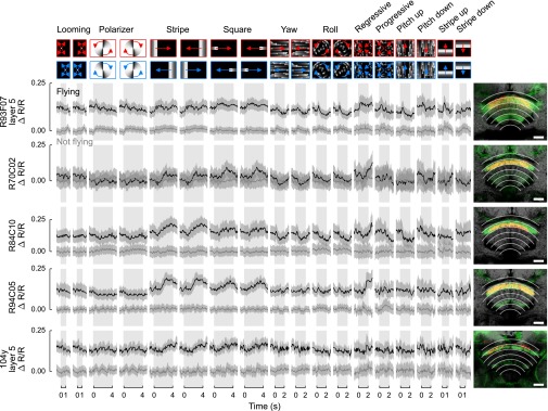
We subjected flies from the driver lines that expressed GCaMP6f and tdTomato in the FB to the same panel of visual stimuli used in our prior experiments and clustered the individual pixels of the image stacks using the same k-means technique applied earlier (Fig. S1). The resulting clusters either spanned the midline, which we termed “tangential response” classes, or they were part of a pair of clusters symmetrical about the midline, which we called “columnar response” classes. We further manually categorized each class as belonging to the ventral, middle, or dorsal third of the FB. We refer to the classes by the names of the GAL4 lines, followed by the layer number if the line revealed response classes in more than one layer. We use the term “type” to refer to biologically distinct kinds of neurons, whereas “classes” are the particular response clusters that we observed using our collection of driver lines. As mentioned above, many of the driver lines we used target more than one cell type; thus, there is not a strict correspondence between type and class. Fig. 5 (Right) shows all of the ventral classes identified in our analysis. We parsed data from columnar class pairs (Fig. 5A) in the same way as we parsed data from the two hemispheres earlier (e.g., the first column of the first row contains data from the left class in response to a looming object on the left and the response of the right class to a looming object on the right.) We pooled the data from tangential classes for pairs of stimuli that were asymmetrical about the midline (first 12 columns), resulting in only six distinct responses (Fig. 5B). Horizontal motion of both small features and large-field patterns (stripe, square, and yaw patterns) elicited strong responses in the ventral FB. These stimulus types are the most important for stabilizing azimuthal heading during flight. Many functional classes responded strongly to regressive (back-to-front) optic flow, although two classes (R49A02 layer 2 and 104y layers 1 and 2) were more strongly responsive to progressive motion. These stimuli simulate the sensory experience of an animal translating backward or forward, and, as such, they would be useful for the control of flight speed in the horizontal plane. In contrast, stimuli useful for controlling elevation or rotation about the pitch and roll axes elicited relatively small responses.

Fig. 5.

Time series data for all individual driver lines with response classes in the ventral third of the FB using the same plotting conventions as in Fig. 2. (Right) Optical sections at the imaging location of neuropil staining in grayscale and GFP expression of the driver line in green from confocal image stacks. Overlaid in red and blue are the results of our clustering algorithm, used to define response classes. (Right, last row) contains only mean tdTomato during the experiment in grayscale. (Scale bars: 20 μm.) (A) Responses of four lines clustered into two columnar classes, one on each side of the midline. (B) Four response classes were tangential, in which one region spanned both sides of the midline. For these data, the responses to either one of the midline-asymmetrical stimulus pairs (first 12 columns) were pooled, so every other column is a reproduction of its neighboring column. (e.g., first and second columns both contain the response to a looming object on either the right or the left). (C) Time series for the two ventral classes of panneuronal data. The purple line is the result of a least-squares fit with nine free scalar parameters (eight weights and one offset) using the eight response classes (shown in A and B) as regressors.

To determine if the responses in these eight functional classes could collectively account for the results in our panneuronal experiments, we performed an ordinary least-squares fit to the panneuronal data using the responses of the classes from the driver lines as independent variables, along with one constant offset variable. The close agreement between the fit and the panneuronal response indicates that the eight functional classes from the individual driver lines are sufficient to recapitulate the responses of all of the cells in the FB (Fig. 5C). We performed this fitting procedure for different numbers of functional classes (from one to eight classes). Perhaps unsurprisingly, the class from the driver line that targeted the largest number of FB cells, R52G12, provided the best fit to the panneuronal data of all of the fits using only a single class (Fig. S4A). The fit provided by R89F06, which only targets 150 FB neurons, provided the second-best fit. A combination of R89F06 and any one of four other classes provided a better fit than R52G12 alone. The fits improved as more classes were added to the algorithm but quickly approached an asymptote. Hence, the observed classes likely contain most, if not all, of the cell types important for processing the panel of visual stimuli during flight in the ventral FB. To test whether this fitting procedure is a meaningful demonstration that the cell classes contained in our collection of driver lines could explain the panneuronal responses, we created 100,000 sets of eight synthetic functional classes in which the responses to each stimulus type were randomly chosen from the set of responses of the eight actual functional classes. We then performed the same fitting procedure on each of these 100,000 synthetic datasets as we did on the actual data. Regardless of how many classes we included in our procedure, the best fits of our actual response classes were significantly better than those fits generated using synthetic classes.

Fig. S4.

Evaluation of goodness of fit for different combinations of response classes. The rms error is plotted for least-squares fits to panneuronal data using all different combinations of observed response classes. R52G12 provided the best fit of all of the fits using only a single class for both ventral and middle layers. All combinations that include R52G12 are shaded green. All combinations that include the second-best single-line fit are shaded blue. All combinations that include both the best and second-best single-line fit are shaded cyan. We added random horizontal offsets to decrease overlap between points. The dark (light) red line indicates the lower 95th (99th) percentile of the fits of a population of synthetic response classes in which responses to each stimulus type were randomly chosen from the set of responses of the actual functional classes (i.e., we randomly chose a row from each column of Figs. 5 and 6 to create synthetic responses). (A) Data for ventral classes (shown in Fig. 5). (B) Data for middle classes (shown in Fig. 6).

Using the same technique as applied to the ventral layers, we found six functional classes in the middle layers of the FB. Three driver lines whose responses all clustered into columnar classes displayed only small-magnitude responses to the stimulus panel (Fig. 6A). The responses of three lines with tangential classes were varied (Fig. 6B). Line 104y, which reportedly only expresses in ventral and dorsal layers, unexpectedly contained cells in the middle layers that responded to horizontal motion. We again performed an ordinary least-squares fit to the panneuronal data using the individual class responses as input variables. The fit was again able to match the qualitative aspects of the middle-layer panneuronal data reasonably well (Fig. 6C and Fig. S4B). Again, horizontal movement of visual features and translational optic flow elicited responses most reliably, indicating that these cells may be involved in regulating heading in azimuth during flight. Five driver lines contained response classes in the dorsal FB (Fig. S5). Although some of these classes displayed flight-induced shifts in baseline fluorescence, none showed significant departures from baseline in response to the stimulus panel.

Fig. 6.

Time series data for all individual driver lines with response classes in the middle third of the FB using the same plotting conventions as in Fig. 5. (Scale bars: 20 μm.) (A) Responses of three lines clustered into two columnar classes, one on each side of the midline. (B) Three response classes were tangential, in which one region spanned both sides of the midline. (C) Time series for middle clusters of panneuronal data (black) and fit (purple) using six middle-response classes as regressors.

Fig. S5.

Time series data for all individual driver lines with response classes in the dorsal third of the FB, using the same plotting conventions as in Figs. 5B and 6B. All these response classes were tangential, and none showed significant stimulus-triggered departures from baseline. (Scale bars: 20 μm.)

Hierarchical Clustering of Responses Reveals Functionally Related Groups.

Several stimuli in our panel elicited similar responses in neurons targeted by different driver lines. To evaluate similarities between lines quantitatively, we hierarchically clustered the responses of all of the functional classes using correlation distance as the distance metric. Fig. S6 shows the resulting dendrogram and distance matrix. Although no anatomical information was available to the clustering algorithm, it nevertheless segregated responses from different anatomical layers with reasonable accuracy, provided we used data collected while the animals were flying. When provided with data from periods when the animals were not flying, the clusters no longer segregated the different layers. There are also several clearly related groups within the layers identified in the flight data. For example, lines R89F06 and R52G12 both contained response classes in the ventral third of the FB, and their responses clustered together, indicating that these two lines likely target many of the same cells. The ventral layer responses were all reasonably similar, with the notable exception of R49A02 in layer 2, which was maximally responsive to progressive optic flow. Additionally, the response of R52G12 in layer 3 was similar to the response of 104y in layers 1 and 2, and both also responded most strongly to progressive optic flow.

Fig. S6.

Analysis of similarity among all FB response classes identified in individual driver lines. Using correlation distance as a distance metric, we clustered the time series for all response classes when the animals were flying (Top) or not flying (Bottom). Three main response types emerge (cyan, magenta, and yellow) in the dendrogram and distance matrix in the responses during flight. These types mostly correspond to anatomical location from our manual annotation (label color on right of distance matrix). (Inset, Upper Right) Mean of all response class pixels colored blue, green, or red according to manual annotation of location in the dorsal, middle, or ventral third of the FB, respectively. To facilitate comparison between flight and nonflight clustering, we colored the leaves of the dendrogram for nonflight data (Bottom) using the same colors as from the flight data (Top).

Discussion

Although the CX has been called a “premotor” area (31), little is known about what types of motor output are controlled by its different substructures. The visual responses we observed in the EB were only slightly enhanced during flight, and those visual responses we observed in the PB were actually suppressed when the animal was flying, suggesting that these regions are involved in processing visual input independent of the behavioral state of the animal. The activity in the FB and NO, however, is strongly contingent on behavioral context, suggesting that these two regions are important for visual control of flight. The lack of correlation with motor response on a trial-by-trial basis (Fig. 3) suggests that the FB and NO neurons are more closely linked to the visual input stream and do not reflect motor commands, efferent copy, or proprioceptive reafference.

The highly structured architecture of the CX has led to much speculation about its function in the insect brain. Anatomically distinguishable layers in the FB exist in many species (2), and a variety of functions have been ascribed to them. In Drosophila, the FB has been reported to contain six, eight, and nine horizontal layers (5, 26, 28), depending on the method used to visualize them. Although there is still uncertainty surrounding their role, this study provides evidence that there are at least three functionally distinct layers. When we imaged activity in the FB using a panneuronal driver and we used a machine-learning algorithm to segment the resulting data, three layers emerged. The ventral and middle layers showed differences across the midline, whereas the dorsal layer was more uniform and relatively unresponsive to our panel of stimuli. Additionally, although no anatomical information other than expression in the FB was used in selecting our diverse collection of driver lines, the response patterns again clustered into three groups that largely adhered to anatomical divisions. These unbiased approaches suggest that the layers are not anatomical epiphenomena but, rather, play distinct roles in visual processing during flight.

The activity in the ventral layers of the FB indicates that the neurons present in this anatomical region can be further subdivided into several functional cell types. Although these neuronal types overlap spatially, their response properties are easily distinguished. The first type, present in both R52G12 and R89F06, is responsive to a variety of visual patterns, including most of those visual patterns in our panel that included horizontal motion. We identified a closely related set in R73D06 and R49A02 layer 1. Neurons in R44B10 and R93F07 layer 2 are more selective for regressive optic flow compared with other types of visual motion. The most functionally distinct subtype in the ventral FB are the cells in both R49A02 layer 2 and line 104y layers 1 and 2, which are selective to progressive optic flow, the opposite to the regressive optic flow preferred by other cells in this region.

Linear combinations of subsets of the eight basic responses that we observed in the ventral FB can recapitulate the panneuronal data, suggesting that these eight classes (or even smaller subsets) are adequate to describe all of the functional responses for the stimuli tested in this study. A similar analysis reveals an even smaller set of responsive classes in the middle layers of the FB. Using photoactivatable GFP, we estimated that over 730 total neurons innervate the FB. The driver lines in our collection contain ∼2.5-fold as many FB neurons, making it probable that each neuronal type is represented more than once, although we cannot be certain that all cell types were included.

We designed the stimulus panel to include a variety of visual patterns that are known to elicit behavioral reactions from flying flies, and verified that the patterns were salient by monitoring behavioral responses simultaneously with neuronal responses. In general, the patterns that elicited the largest neuronal responses contained horizontal motion. This type of optic flow is essential for steering in the azimuthal plane, suggesting that the FB is involved in the visual processing necessary for stabilizing heading during flight. A special type of stimulus motion, translational optic flow, is experienced when an agent translates through a visual scene (32). When an animal translates forward, its movement creates front-to-back motion on the retina, termed “progressive optic flow,” whereas backward translation creates regressive optic flow. Our observation of neurons responsive to both of these types of visual motion suggests that the FB may also play a role in the regulation of forward flight speed. The remarkable ability of some flying insects to measure distances traveled by measuring a path integral of progressive optic flow (33) must rely on neurons, like those neurons observed in this study, that respond to progressive visual stimuli during flight.

Unlike contrast-based stimuli, the polarized light stimulus in our panel did not elicit large neuronal responses in any of the driver lines we studied. In preliminary experiments, we verified that this same stimulus was sufficient to elicit neuronal responses in the optic lobes, and previous studies have shown that flies respond behaviorally to changes in the polarization angle of light (34–36). Unlike the FB, the EB and PB have been implicated in extensive involvement in the analysis of polarization information in other species, and a more detailed analysis of those structures is warranted.

Because neurons in the FB only respond to visual stimuli when the animal is flying, they must receive input about both the external state of the visual surround and the current behavioral state of the animal. Although we did not observe any correlation with behavior other than the large increase in baseline during flight, it is likely that the FB is a site of interaction between sensory input and motor output, consistent with the recent finding that it is one of the most highly connected neuropils in the Drosophila brain (31). Functional responses in NO neurons are similar to functional responses in FB cells, indicating that they may also be involved in the control of flight direction. Activity in the PB increases during flight, and we observed translational symmetry across the midline of functional regions. Neurons in the EB have been shown to respond to visual features in small receptive fields (19) and to encode head direction in walking flies (21).

Most work on the functional responses of CX neurons has been done in restrained animals, whereas behavioral studies often rely on ablation or silencing techniques to deduce neuronal function. The advent of techniques for visualizing neuronal responses in behaving animals (37–39) made it possible to observe flight-dependent responses to visual motion in the central brain. In Fig. S6 (Lower), we reproduced the clustering of response classes using data from periods of quiescence instead of periods when the animals were flying. The resulting clusters are largely different and considerably less separated than the flight clusters, and some have disappeared altogether. Thus, responses of the FB to identical stimuli are fundamentally different when the animal is engaged in different behaviors. This example of state dependence in the functional connectivity of a circuit indicates a limitation of connectomics based purely on anatomy and provides a starting point for future studies. We can now directly observe the bulk activity of a neuronal population during naturalistic behavior and discover the genetically defined cell types that constitute that functional population.

Materials and Methods

Flies.

All flies included in this study were adult females no more than 8 d after eclosion. They were raised at 25 °C on standard cornmeal medium on a 16:8-h light/dark cycle. We prepared flies using previously published techniques (37). Briefly, we chilled flies to 4 °C, removed all legs (to promote flight), and then used UV-curing glue to affix them to custom stages. Immediately before each experiment, we used a hypodermic needle to dissect a small hole in the center of the posterior cuticle of the head in saline. Throughout the experiment, we perfused the brain with 19 °C saline. The following fly stocks were used (the numbers in brackets indicate the number of individual flies tested in our imaging experiments for each FB driver line): 104y-GAL4 (30) [5], R12G01-GAL4 [no expression], R14E06-GAL4 [6], R38E07-GAL4 [8], R42B05-GAL4 [5], R44B10-GAL4 [6], R49A02-GAL4 [5], R52G12-GAL4 [9], R70C02-GAL4 [4], R73D06-GAL4 [7], R75G12-GAL4 [no expression], R84C10-GAL4 [6], R89F06-GAL4 [5], R93F07-GAL4 [4], R94C05-GAL4 [4], R95F02-GAL4 (29) [5], panneuronal R57C10-GAL4 (25), UAS-GCaMP6f (23), UAS-tdTomato (24), and UAS-PA-GFP (40). Fifteen original lines met the search criteria we used in selecting driver lines from the FlyLight collection, but two lines showed no signal in the targeted region when we independently examined them using tdTomato and GCaMP6f expression.

Stimuli.

An array spanning ±108° horizontally from the fly’s midline (96 total pixels) and ±32° vertically from the fly’s horizon (32 total pixels) of blue light-emitting diodes (LEDs; 470-nm peak wavelength) displayed 16 visual patterns. Three layers of blue filter (Rosco no. 59 indigo) prevented light from this array from leaking into the photomultiplier tubes used for imaging fluorescence and shifted the spectral peak to ∼454 nm. Each LED in this array contributed ∼1 nW⋅cm⁻² flux at the location of the fly when illuminated. An animation showing all of the stimuli is available for downloading (Movie S2). In addition, two stimuli consisted of a UV LED (365-nm peak wavelength, filtered with a 400-nm short-pass filter) illuminating three ground-glass diffusers for 4 s. The light from these diffusers projected through a linearly polarizing filter that rotated at ±45° per second. This filter arrangement resulted in light with an average wavelength of ∼378 nm and intensity of 0.73 μW⋅cm⁻² reaching the location of the fly. We presented the stimuli in random order. Between stimuli, all of the LEDs were dark for 2 s. To elicit flight, we delivered 200-ms puffs of air at the fly from a vacuum pump (Cole–Parmer). We presented eight repetitions of all of the stimuli while the animal was not flying and eight repetitions when the animal was flying. In later analysis, we discarded trials during which the fly stopped or started flying or we delivered an air puff.

Flight Behavior.

Two IR LEDs (850-nm peak wavelength) illuminated the fly via optical fibers. An IR-sensitive camera (Basler) recorded movies of the fly from below at 40 frames per second. From these movies, an automated machine vision routine (37) extracted and saved the left and right wing stroke amplitudes.

Functional Imaging.

We used a Nikon 40× NIR Apo objective water-immersion lens (0.8 N.A.) with a Prairie Ultima IV multiphoton microscope to record fluorescence of GCaMP6f and tdTomato in images with pixels sized 0.66 × 0.66 μm. A 930-nm Ti:Sapphire laser (Coherent) provided between 15 and 27 mW (depending on the line’s expression intensity) at the back aperture of the objective lens and dwelled on each pixel for 4 μs. Frame rates varied from 9.5 to 20.8 frames per second, depending on the size of the region of interest. Two multialkali photomultiplier tubes collected fluorescence simultaneously after it was band-passed by either an HQ 525/50m-2p or HQ 607/45-2p emission filter (Chroma Technology).

Analysis.

We analyzed the functional imaging data with custom scripts written in Python and created plots using Matplotlib (41). Before each experiment, we acquired a full-frame (512 × 512 pixels) anatomical reference of the tdTomato signal at the imaging depth, to which we rigidly registered the tdTomato channel of every frame to within the nearest pixel by finding the peak of the cross-correlation between the two images.

To find pixels in the imaging frames that responded similarly, we subtracted the mean of the GCaMP6f frames 1 s before each trial during which flies flew from the mean during stimulus motion. We used the k-means algorithm to cluster the pixels in these difference images (42). To determine the number of clusters used in later analysis, we used both a condition for bilateral symmetry of the derived clusters and the silhouette coefficient score (27), an average distance between the points of a cluster and the closest neighboring clusters normalized to the average intracluster distance (1 indicates perfect clustering, −1 is the worst possible score) (Fig. S1). After identifying clusters of pixels, we computed the ratio R_t of GCaMP6f fluorescence to tdTomato fluorescence in each cluster for every time point t. For each cluster, we computed the mean baseline ratio R₀ during the 1 s before stimulus motion for all trials when the animal was not flying. We plot the difference between the instantaneous ratio of fluorescence and this baseline ratio normalized to the baseline ratio for time-series data, (R_t − R₀)/R₀, which we term “ΔR/R.” Dividing the GCaMP6f fluorescence by the tdTomato fluorescence decreased the effect of movements in depth, because such movements result in correlated changes in both signals. (Such changes would be indistinguishable from changes in GCaMP6f fluorescence if that signal were not normalized to tdTomato fluorescence.) We calculated 95% confidence intervals around the mean ΔR/R for each trial type by creating 500,000 random bootstrap resamples with replacement of all of the original individual responses and then finding the 2.5 and 97.5 percentiles of the resulting distribution.

As a conservative measure of significance, we used the Mann–Whitney U test to compare the mean R_t during 1 s prestimulus and the mean R_t during the stimulus. We corrected for multiple comparisons using the Bonferroni correction based on the product of the number of trial types (18), behavioral states (2), and response classes (four in Fig. 2, nine in Fig. 5, seven in Fig. 6, and five in Fig. S5). If a response after correction was significant at the P < 0.05 level, we colored the confidence interval of that trace yellow. This method for determining significance is conservative for several reasons. First, we corrected for the largest reasonable number of comparisons, at least 144, possible in each figure, although it is probable that only a subset of those comparisons is of interest. Second, the Bonferroni correction itself is a conservative approach to correct for multiple comparisons. Finally, it is possible that responses to stimuli were transiently high (or low) but that the mean across the entire stimulus period was not significantly increased (or decreased). We used this conservative method to avoid false-positive results but presented time-series data for all experiments to show the details of responses that failed to meet this stringent criterion.

We used the ordinary least-squares approach to determine if a linear combination of the individual functional class responses could recapitulate the panneuronal response. For each class, we concatenated the mean flight response to each stimulus (i.e., we concatenated the columns of each row in Figs. 5 and 6). The resulting vectors, in addition to one constant offset term, served as the regressors. For the eight ventral classes, this analysis yielded nine scalar quantities, eight of which represent weights. The sum of all of the class responses weighted by these scalars provides a fit to the panneuronal response (by minimizing the sum squared error between the fit and the measured panneuronal response). We plotted the predicted vector with the actual panneuronal data vector to demonstrate the fit. We analyzed all subsets of our response classes in Fig. S4 to evaluate how well different numbers of classes were able to recapitulate the panneuronal responses. To evaluate the closeness of the fits, we created a population of synthetic responses by choosing randomly one class response for each trial type from our observed class responses and concatenating these randomly selected responses. We then performed a least-squares fit to the panneuronal data using our synthetic response population as regressors. By repeating this process 100,000 times, we found the 95th and 99th percentiles of fits that could be expected based on chance and the temporal dynamics common to our entire dataset.

The responses of functional classes from different driver lines often resembled one another. To cluster the responses and make predictions about which lines contained overlapping sets of neurons, we created a dendrogram of response similarity. We used the concatenated mean response vector for each class (discussed above) and the unweighted pair group method with arithmetic mean algorithm to construct this dendrogram. We used the correlation distance as the distance metric:

$$D=1\mathrm{-}\frac{\left(u\mathrm{-}\overline{u}\right)\mathrm{\cdot }\left(v\mathrm{-}\overline{v}\right)}{{\Vert \left(u\mathrm{-}\overline{u}\right)\Vert }_2{\Vert \left(v\mathrm{-}\overline{v}\right)\Vert }_2},$$ [1]

where D is the correlation distance between vectors u and v, and ū denotes the mean of the elements of u. We also plotted a heat map of this distance metric.

Cell Counting.

To count neurons with processes in the FB, we expressed PA-GFP and tdTomato with the panneuronal driver R57C10-GAL4. Using the tdTomato signal to find the region of interest, we activated the FB by illuminating a 160 × 108-pixel region 8,800 times, in blocks of 32 separated by 10-s intervals. We used 750-nm laser light at 30 mW (measured at the back aperture of the objective lens). Before and after photoactivation, we acquired z-stacks of images with 0.33 × 0.33-μm pixels in steps of 1 μm using 930-nm light. We used the tdTomato channel to align the first z-stack to the second z-stack with the BrainAligner (43) algorithm. By using the Synchronize Windows function in ImageJ (NIH), we could scroll through the aligned stacks simultaneously and count somata of neurons containing photoactivated GFP using the Cell Counter plug-in. We performed this analysis separately for the region of the brain posterior to the FB (three animals) and the region anterior to the FB (two animals) to avoid loss of resolution as we imaged through more tissue. We also used the Cell Counter plug-in to count somata in the confocal image stacks of the driver lines used in this study. We used the variance between somata counts in the left and right hemispheres to estimate variance in this measurement.

References

- 1.Loesel R, Nässel DR, Strausfeld NJ. Common design in a unique midline neuropil in the brains of arthropods. Arthropod Struct Dev. 2002;31(1):77–91. doi: 10.1016/S1467-8039(02)00017-8. [DOI] [PubMed] [Google Scholar]
- 2.Homberg U. Evolution of the central complex in the arthropod brain with respect to the visual system. Arthropod Struct Dev. 2008;37(5):347–362. doi: 10.1016/j.asd.2008.01.008. [DOI] [PubMed] [Google Scholar]
- 3.Heinze S, Homberg U. Neuroarchitecture of the central complex of the desert locust: Intrinsic and columnar neurons. J Comp Neurol. 2008;511(4):454–478. doi: 10.1002/cne.21842. [DOI] [PubMed] [Google Scholar]
- 4.Lin C-Y, et al. A comprehensive wiring diagram of the protocerebral bridge for visual information processing in the Drosophila brain. Cell Reports. 2013;3(5):1739–1753. doi: 10.1016/j.celrep.2013.04.022. [DOI] [PubMed] [Google Scholar]
- 5.Wolff T, Iyer NA, Rubin GM. Neuroarchitecture and neuroanatomy of the Drosophila central complex: A GAL4-based dissection of protocerebral bridge neurons and circuits. J Comp Neurol. 2015;523(7):997–1037. doi: 10.1002/cne.23705. [DOI] [PMC free article] [PubMed] [Google Scholar]
- 6.Vitzthum H, Muller M, Homberg U. Neurons of the central complex of the locust Schistocerca gregaria are sensitive to polarized light. J Neurosci. 2002;22(3):1114–1125. doi: 10.1523/JNEUROSCI.22-03-01114.2002. [DOI] [PMC free article] [PubMed] [Google Scholar]
- 7.Heinze S, Homberg U. Linking the input to the output: New sets of neurons complement the polarization vision network in the locust central complex. J Neurosci. 2009;29(15):4911–4921. doi: 10.1523/JNEUROSCI.0332-09.2009. [DOI] [PMC free article] [PubMed] [Google Scholar]
- 8.Rosner R, Homberg U. Widespread sensitivity to looming stimuli and small moving objects in the central complex of an insect brain. J Neurosci. 2013;33(19):8122–8133. doi: 10.1523/JNEUROSCI.5390-12.2013. [DOI] [PMC free article] [PubMed] [Google Scholar]
- 9.Kathman ND, Kesavan M, Ritzmann RE. Encoding wide-field motion and direction in the central complex of the cockroach Blaberus discoidalis. J Exp Biol. 2014;217(Pt 22):4079–4090. doi: 10.1242/jeb.112391. [DOI] [PubMed] [Google Scholar]
- 10.Ritzmann RE, Ridgel AL, Pollack AJ. Multi-unit recording of antennal mechano-sensitive units in the central complex of the cockroach, Blaberus discoidalis. J Comp Physiol A Neuroethol Sens Neural Behav Physiol. 2008;194(4):341–360. doi: 10.1007/s00359-007-0310-2. [DOI] [PubMed] [Google Scholar]
- 11.Guo P, Ritzmann RE. Neural activity in the central complex of the cockroach brain is linked to turning behaviors. J Exp Biol. 2013;216(Pt 6):992–1002. doi: 10.1242/jeb.080473. [DOI] [PubMed] [Google Scholar]
- 12.Bender JA, Pollack AJ, Ritzmann RE. Neural activity in the central complex of the insect brain is linked to locomotor changes. Curr Biol. 2010;20(10):921–926. doi: 10.1016/j.cub.2010.03.054. [DOI] [PubMed] [Google Scholar]
- 13.Kahsai L, Martin J-R, Winther AM. Neuropeptides in the Drosophila central complex in modulation of locomotor behavior. J Exp Biol. 2010;213(Pt 13):2256–2265. doi: 10.1242/jeb.043190. [DOI] [PubMed] [Google Scholar]
- 14.Triphan T, Poeck B, Neuser K, Strauss R. Visual targeting of motor actions in climbing Drosophila. Curr Biol. 2010;20(7):663–668. doi: 10.1016/j.cub.2010.02.055. [DOI] [PubMed] [Google Scholar]
- 15.Neuser K, Triphan T, Mronz M, Poeck B, Strauss R. Analysis of a spatial orientation memory in Drosophila. Nature. 2008;453(7199):1244–1247. doi: 10.1038/nature07003. [DOI] [PubMed] [Google Scholar]
- 16.Ofstad TA, Zuker CS, Reiser MB. Visual place learning in Drosophila melanogaster. Nature. 2011;474(7350):204–207. doi: 10.1038/nature10131. [DOI] [PMC free article] [PubMed] [Google Scholar]
- 17.Liu G, et al. Distinct memory traces for two visual features in the Drosophila brain. Nature. 2006;439(7076):551–556. doi: 10.1038/nature04381. [DOI] [PubMed] [Google Scholar]
- 18.Bausenwein B, Müller NR, Heisenberg M. Behavior-dependent activity labeling in the central complex of Drosophila during controlled visual stimulation. J Comp Neurol. 1994;340(2):255–268. doi: 10.1002/cne.903400210. [DOI] [PubMed] [Google Scholar]
- 19.Seelig JD, Jayaraman V. Feature detection and orientation tuning in the Drosophila central complex. Nature. 2013;503(7475):262–266. doi: 10.1038/nature12601. [DOI] [PMC free article] [PubMed] [Google Scholar]
- 20.Weir PT, Schnell B, Dickinson MH. Central complex neurons exhibit behaviorally gated responses to visual motion in Drosophila. J Neurophysiol. 2014;111(1):62–71. doi: 10.1152/jn.00593.2013. [DOI] [PubMed] [Google Scholar]
- 21.Seelig JD, Jayaraman V. Neural dynamics for landmark orientation and angular path integration. Nature. 2015;521(7551):186–191. doi: 10.1038/nature14446. [DOI] [PMC free article] [PubMed] [Google Scholar]
- 22.Muijres FT, Elzinga MJ, Iwasaki NA, Dickinson MH. Body saccades of Drosophila consist of stereotyped banked turns. J Exp Biol. 2015;218(Pt 6):864–875. doi: 10.1242/jeb.114280. [DOI] [PubMed] [Google Scholar]
- 23.Chen TW, et al. Ultrasensitive fluorescent proteins for imaging neuronal activity. Nature. 2013;499(7458):295–300. doi: 10.1038/nature12354. [DOI] [PMC free article] [PubMed] [Google Scholar]
- 24.Shaner NC, et al. Improved monomeric red, orange and yellow fluorescent proteins derived from Discosoma sp. red fluorescent protein. Nat Biotechnol. 2004;22(12):1567–1572. doi: 10.1038/nbt1037. [DOI] [PubMed] [Google Scholar]
- 25.Henry GL, Davis FP, Picard S, Eddy SR. Cell type-specific genomics of Drosophila neurons. Nucleic Acids Res. 2012;40(19):9691–9704. doi: 10.1093/nar/gks671. [DOI] [PMC free article] [PubMed] [Google Scholar]
- 26.Hanesch U, Fischbach K, Heisenberg M. Neuronal architecture of the central complex in Drosophila melanogaster. Cell Tissue Res. 1989;257(257):343–366. [Google Scholar]
- 27.Rousseeuw PJ. Silhouettes: A graphical aid to the interpretation and validation of cluster analysis. J Comput Appl Math. 1987;20:53–65. [Google Scholar]
- 28.Young JM, Armstrong JD. Structure of the adult central complex in Drosophila: Organization of distinct neuronal subsets. J Comp Neurol. 2010;518(9):1500–1524. doi: 10.1002/cne.22284. [DOI] [PubMed] [Google Scholar]
- 29.Jenett A, et al. A GAL4-driver line resource for Drosophila neurobiology. Cell Reports. 2012;2(4):991–1001. doi: 10.1016/j.celrep.2012.09.011. [DOI] [PMC free article] [PubMed] [Google Scholar]
- 30.Yang MY, Armstrong JD, Vilinsky I, Strausfeld NJ, Kaiser K. Subdivision of the Drosophila mushroom bodies by enhancer-trap expression patterns. Neuron. 1995;15(1):45–54. doi: 10.1016/0896-6273(95)90063-2. [DOI] [PubMed] [Google Scholar]
- 31.Shih C-T, et al. Connectomics-based analysis of information flow in the Drosophila brain. Curr Biol. 2015;25(10):1249–1258. doi: 10.1016/j.cub.2015.03.021. [DOI] [PubMed] [Google Scholar]
- 32.Gibson JJ. Visually controlled locomotion and visual orientation in animals. Br J Psychol. 1958;49(3):182–194. doi: 10.1111/j.2044-8295.1958.tb00656.x. [DOI] [PubMed] [Google Scholar]
- 33.Esch H, Burns J. Distance estimation by foraging honeybees. J Exp Biol. 1996;199(Pt 1):155–162. doi: 10.1242/jeb.199.1.155. [DOI] [PubMed] [Google Scholar]
- 34.Wolf R, Gebhardt B, Gademann R, Heisenberg M. Polarization sensitivity of course control in Drosophila melanogaster. J Comp Physiol A Neuroethol Sens Neural Behav Physiol. 1980;139:177–191. [Google Scholar]
- 35.Weir PT, Dickinson MH. Flying Drosophila orient to sky polarization. Curr Biol. 2012;22(1):21–27. doi: 10.1016/j.cub.2011.11.026. [DOI] [PMC free article] [PubMed] [Google Scholar]
- 36.Wernet MF, et al. Genetic dissection reveals two separate retinal substrates for polarization vision in Drosophila. Curr Biol. 2012;22(1):12–20. doi: 10.1016/j.cub.2011.11.028. [DOI] [PMC free article] [PubMed] [Google Scholar]
- 37.Maimon G, Straw AD, Dickinson MH. Active flight increases the gain of visual motion processing in Drosophila. Nat Neurosci. 2010;13(3):393–399. doi: 10.1038/nn.2492. [DOI] [PubMed] [Google Scholar]
- 38.Suver MP, Mamiya A, Dickinson MH. Octopamine neurons mediate flight-induced modulation of visual processing in Drosophila. Curr Biol. 2012;22(24):2294–2302. doi: 10.1016/j.cub.2012.10.034. [DOI] [PubMed] [Google Scholar]
- 39.Seelig JD, et al. Two-photon calcium imaging from head-fixed Drosophila during optomotor walking behavior. Nat Methods. 2010;7(7):535–540. doi: 10.1038/nmeth.1468. [DOI] [PMC free article] [PubMed] [Google Scholar]
- 40.Patterson GH, Lippincott-Schwartz J. A photoactivatable GFP for selective photolabeling of proteins and cells. Science. 2002;297(5588):1873–1877. doi: 10.1126/science.1074952. [DOI] [PubMed] [Google Scholar]
- 41.Hunter JD. Matplotlib: A 2D graphics environment. Comput Sci Eng. 2007;9(3):90–95. [Google Scholar]
- 42.Pedregosa F, et al. Scikit-learn: Machine learning in Python. J Mach Learn Res. 2011;12:2825–2830. [Google Scholar]
- 43.Peng H, et al. BrainAligner: 3D registration atlases of Drosophila brains. Nat Methods. 2011;8(6):493–500. doi: 10.1038/nmeth.1602. [DOI] [PMC free article] [PubMed] [Google Scholar]
Associated Data
This section collects any data citations, data availability statements, or supplementary materials included in this article.