A 3D Primary Vessel Reconstruction Framework with Serial Microscopy Images

Abstract

Three dimensional microscopy images present significant potential to enhance biomedical studies. This paper presents an automated method for quantitative analysis of 3D primary vessel structures with histology whole slide images. With registered microscopy images of liver tissue, we identify primary vessels with an improved variational level set framework at each 2D slide. We propose a Vessel Directed Fitting Energy (VDFE) to provide prior information on vessel wall probability in an energy minimization paradigm. We find the optimal vessel cross-section associations along the image sequence with a two-stage procedure. Vessel mappings are first found between each pair of adjacent slides with a similarity function for four association cases. These bi-slide vessel components are further linked by Bayesian Maximum A Posteriori (MAP) estimation where the posterior probability is modeled as a Markov chain. The efficacy of the proposed method is demonstrated with 54 whole slide microscopy images of sequential sections from a human liver.

1 Introduction

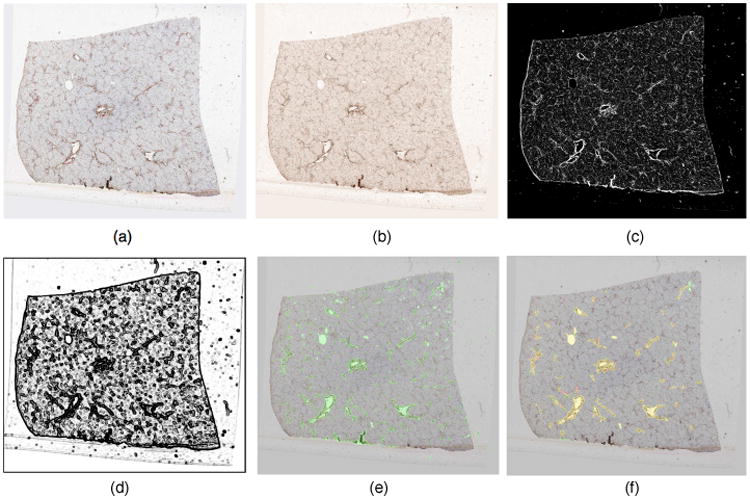
Whole slide histological images contain rich information about morphological and pathological characteristics of biological systems, enabling researchers and clinicians to gain insights on the underlying mechanisms of the disease onsets and pathological evolutions of distinct cancers. Although numerous imaging analytical approaches have been proposed to quantitatively analyze the 2D biological structures (such as nuclei and vessels) in microscopy images [1], various clinical applications require 3D modeling of the micro-anatomic objects for better characterization of their biological structures in practice. One such application is liver disease where clinicians and researchers are interested in the 3D structural features of primary vessels from a sequence of 2D images of adjacent liver sections [2, 3], as illustrated in Fig. 1(a). Although there are a large suite of methods for vessel structure analysis, they mainly focus on radiology image analysis and are not directly applicable to high resolution whole slide histological images encoding enormous information of complex structures at cellular level.

Fig 1.

Representative segmentation result of primary vessels. (a) a typical 2D liver histology image with vessels highlighted in brown; (b) DAB stain image channel derived from color deconvolution; (c) vessel wall probability map P(x); (d) smooth indicator function Q_σ3(x); (e) segmented primary vessels after post-processing (in green); and (f) markup image with one-to-one vessel pairs by human (red) and machine (green), with yellow mask resulting from red and green mask.

In this paper, we propose an automated framework for 3D primary vessel reconstruction with a set of registered histological whole slide images of liver sequential tissue sections. To identify vessels, we use an improved variational level set method with a Vessel Directed Fitting Energy (VDFE) as prior information of vessel wall probability for the energy minimization paradigm. We associate the segmented vessel objects across all slides by mapping primary vessels between adjacent slides with four distinct association scenarios, and apply a Bayesian Maximum A Posteriori (MAP) framework to the bi-slide vessel components to recover the global vessel structures across all slides.

2 Methods for 3D Vessel Reconstruction

2.1 Automated 2D Vessel Segmentation

Due to large variations introduced by whole slide microscopy image preparation and strong heterogeneity embedded in tissue anatomical structures, vessels of interest in liver biopsies present distinct staining intensities. Although a number of level set methods have been proposed to solve this issue [4, 5], these formulations only work well when a given image has two primary classes of connected regions. In our dataset, each typical liver image consists of primary vessel walls, lumens, small vessel walls, bile ducts, and non-tissue regions, each presenting different intensity characteristics. One solution is to employ multiple fitting functions to reach functional minimum [5]. However, this would inevitably increase the computational complexity. As we focus on identifying primary vessel walls in this work, we propose an improved formulation with directed prior information on vessel wall probability within a variational level set framework based on [5]. Let us denote two 2D vectors x and y defined over the image domain Ω of image I. Level set ϕ : Ω → ℛ is a Lipschitz function defined over Ω. Vessel Directed Fitting Energy (VDFE) E_V is then defined as follows:

$$E_{\mathrm{V}}(\mathbf{x},f_1,f_2,\varphi )={\lambda }_1{\int }_{\Omega }{G}_{{\sigma }_2}(\Vert \mathbf{x}-\mathbf{y}\Vert )Q_{{\sigma }_3}(\mathbf{y}){|I(\mathbf{y})\ast G_{{\sigma }_1}(\mathbf{y})-f_1(\mathbf{x})|}^2{U}_1(\varphi (\mathbf{y}))d\mathbf{y}+{\lambda }_2{\int }_{\Omega }{G}_{{\sigma }_2}(\Vert \mathbf{x}-\mathbf{y}\Vert )P(\mathbf{y}){|I(\mathbf{y})\ast G_{{\sigma }_1}(\mathbf{y})-f_2(\mathbf{x})|}^2{U}_2(\varphi (\mathbf{y}))d\mathbf{y}$$ (1)

where f₁ (x) and f₂ (x) are two fitting functions for interior and exterior regions of zero level set. G_σ is a bivariate Gaussian filter; $U_i(\varphi (\mathbf{x}))=\{\begin{array}{cc}H(\varphi (\mathbf{x})),& \text{if}i=1\\ 1-H(\varphi (\mathbf{x})),& \text{if}i=2\end{array}$ and H (x) is a Heaviside step function; $Q_{\sigma }(\mathbf{x})=exp(-\frac{{|\mathrm{\nabla }\mathbf{x}|}^2}{2{\sigma }^2})$ is a function describing image smoothness. P(y) = max p(y, s_i, τ, ω) is a pre-computed vessel wall probability map indicating the likelihood of pixel y belonging to a vessel wall [6] where s_i is the i^th scale of a Gaussian filter that convolves with the image channel representing vessel-specific immunohistochemical stain DAB [7]; τ and ω are parameters governing the sensitivity of P(y) to measures of vessel structure similarity and intensity change magnitude. We set τ = 0.5 and ω = 15.

In our formulation, fitting function f₁(x) fits better to y in close proximity to x and with large Q_σ3(y). Similarly, f₂(x) is biased to image locations y close to x and with large P(y). Compared with small vessels, primary vessels have longer edge contours where Q_σ3 (y) is low. Thus, VDFE minimization guarantees that f₁(x) is automatically elected to fit to primary vessel wall regions where Q_σ3 (y) is small and that f₂ (x) fits to non-primary vessel regions where P (y) is small. Therefore, the proposed VDFE uses joint information derived from image regions, vessel edges, and the prior vessel wall probability map. To regulate zero level set smoothness, and retain signed distance property for stable level set function computation, we use the following accessory energy terms [8]: E₁(ϕ(x)) = αQ_σ3 (x)|∇H(ϕ(x))| and E₂(ϕ(x)) = βR(|∇ϕ(x)|). In addition, we introduce another energy term to expedite zero level set convergence to vessel walls: E₃(ϕ(x)) = γ (1 − P(x)) H (ϕ(x)). Combining all energies, we formulate the following functional to be minimized:

$$\mathcal{J}(f_1(\mathbf{x}),f_2(\mathbf{x}),\varphi )={\int }_{\Omega }[E_{\mathrm{V}}(\mathbf{x},f_1(\mathbf{x}),f_2(\mathbf{x}),\varphi )+\sum _{i=1}^3{E}_i(\varphi (\mathbf{x}))]d\mathbf{x}$$ (2)

We update f₁, f₂, and ϕ in two sequential steps within each iteration as suggested by the local binary fitting model [5]. First, we fix ϕ(x) and optimize f₁ (x) and f₂ (x) to minimize functional by solving the system of Euler-Lagrange equations. Next, we minimize functional ℐ by optimizing ϕ(x) with two updated fitting functions unchanged. Note that we can swap integration variables x and y, change the integration order for the energy term E_V, and re-write the integrand:

$$\mathcal{L}(\mathbf{x},\varphi (\mathbf{x}))={\lambda }_1\underset{\text{defined as}:F_1(\mathbf{x})}{\underbrace{{\int }_{\Omega }{G}_{{\sigma }_2}(\Vert \mathbf{y}-\mathbf{x}\Vert ){|I(\mathbf{x})\ast G_{{\sigma }_1}(\mathbf{x})-f_1^{\ast }(\mathbf{y})|}^{2}d\mathbf{y}}}{Q}_{{\sigma }_3}(\mathbf{x})H(\varphi (\mathbf{x}))+{\lambda }_2\underset{\text{defined as}:F_2(\mathbf{x})}{\underbrace{{\int }_{\Omega }{G}_{{\sigma }_2}(\Vert \mathbf{y}-\mathbf{x}\Vert ){|I(\mathbf{x})\ast G_{{\sigma }_1}(\mathbf{x})-f_2^{\ast }(\mathbf{y})|}^{2}d\mathbf{y}}}P(\mathbf{x})(1-H(\varphi (\mathbf{x})))+\alpha Q_{{\sigma }_3}(\mathbf{x})|\mathrm{\nabla }H(\varphi (\mathbf{x}))|+\beta R(|\mathrm{\nabla }\varphi (\mathbf{x})|)+\gamma (1-P(\mathbf{x}))H(\varphi (\mathbf{x}))$$

By the Euler-Lagrange equation, we have the final updating equation as:

$$\frac{\partial \varphi (\mathbf{x};t)}{\partial t}=-\frac{\partial \mathcal{J}(\varphi )}{\partial \varphi }=-\frac{\partial \mathcal{L}(\mathbf{x},\varphi (\mathbf{x}))}{\partial \varphi (\mathbf{x})}+\sum _{i=1}^2\frac{\partial }{\partial x_i}\left(\frac{\partial \mathcal{L}(\mathbf{x},\varphi (\mathbf{x}))}{\frac{\partial \varphi (\mathbf{x})}{\partial x_i}}\right)=[{\lambda }_2{F}_2(\mathbf{x})P(\mathbf{x})-{\lambda }_1{F}_1(\mathbf{x})Q_{{\sigma }_3}(\mathbf{x})]H\prime (\mathbf{x})+\alpha [\mathrm{\nabla }{Q}_{{\sigma }_3}(\mathbf{x})\cdot \frac{\mathrm{\nabla }\varphi (\mathbf{x})}{|\mathrm{\nabla }\varphi (\mathbf{x})|}+Q_{{\sigma }_3}(\mathbf{x})\mathrm{d}iv(\frac{\mathrm{\nabla }\varphi (\mathbf{x})}{|\mathrm{\nabla }\varphi (\mathbf{x})|})]H\prime (\mathbf{x})+\beta \mathrm{d}iv(\frac{R\prime (|\mathrm{\nabla }\varphi (\mathbf{x})|)}{|\mathrm{\nabla }\varphi (\mathbf{x})|}\mathrm{\nabla }\varphi (\mathbf{x}))-\gamma (1-P(x))H\prime (\varphi (x))$$ (3)

2.2 Two-stage Vessel Association with Vessel Cross-sections

We perform vessel association by two steps: local bi-slide vessel mapping and global vessel structure association. At each stage, we consider four different association cases: one-to-one (growth), one-to-two (bifurcation), one-to-none (disappearance) and none-to-one (appearance). For local bi-slide vessel mapping, we take into account vessel shape descriptors and spatial features, with the overall similarity function for each association case defined as follows:

1. One-to-one: $s({\upsilon }_i^t,{\upsilon }_j^{t+1})={\mu }_{1}g({\upsilon }_i^t,{\upsilon }_j^{t+1})+{\mu }_{2}d({\upsilon }_i^t,{\upsilon }_j^{t+1})$

2. One-to-two: $s({\upsilon }_i^t,{\upsilon }_{j_1}^{t+1},{\upsilon }_{j_2}^{t+1})={\mu }_{1}g({\upsilon }_i^t,{\upsilon }_{j_1}^{t+1}\cup {\upsilon }_{j_2}^{t+1})+{\mu }_{2}d({\upsilon }_i^t,{\upsilon }_{j_1}^{t+1}\cup {\upsilon }_{j_2}^{t+1})$

3. One-to-none: $s({\upsilon }_i^t,{\upsilon }_{\mathrm{\varnothing }}^{t+1})=d({\upsilon }_i^t,{\Omega }_t)$

4. None-to-one: $s({\upsilon }_{\mathrm{\varnothing }}^{t-1},{\upsilon }_i^t)=d({\upsilon }_i^t,O_t)$

where ${\upsilon }_i^t$ is the i^th vessel object in slide t; functions g(·) and d(·) are two Gaussian Radial Basis Functions (GRBF) with scale κ₁ and κ₂, representing the similarity of vessel appearance by Fourier shape descriptors and the spatial distance between two vessel objects, respectively; Ω_t and O_t are the boundary and centroid of slide t; {μ₁, μ₂} with μ₁ + μ₂ = 1 are constant weights to control the bi-slide vessel mapping smoothness.

The bi-slide vessel mapping is considered as a multi-object tracking problem, and solved by constrained Integer Programming [9] based on the defined similarity functions. This stage generates a set of bi-slide vessel components B = {B_i}. Next, we reconstruct the global vessel structures by linking {B_i} across all slides within a Bayesian Maximum A Posteriori (MAP) framework [10, 11]. Denote V = {V_k} as the set of hypotheses on vessel structures over all slides. Each vessel structure V_k may contain the pre-defined four association cases and can be written as $V_k=\{B_i^k\}$ where $B_i^k$ is the ith bi-slide vessel component in vessel structure V_k. $B_i^k$ can be represented as $B_i^k=({\upsilon }_{p\prime }^k\to {\upsilon }_p^k)$ where ${\upsilon }_{p\prime }^k$, and ${\upsilon }_p^k$ are the associated vessel objects linked by $B_i^k$. We maximize the following marginal posterior probability to obtain the best vessel structure hypothesis V*:

$$\mathbf{V}\ast =arg\underset{\mathbf{V}}{max}P(\mathbf{V}|\mathbf{B})=arg\underset{\mathbf{V}}{max}\prod _{V_k\in \mathbf{V}}P(V_k|\mathbf{B})=\underset{B_s^k\in V_k}{P_{\mathrm{\varnothing }\to 1}}(B_s^k|B_{\mathrm{\varnothing }})\prod _{B_i^k,B_j^k\in V_k}{P}_{1\to 1}(B_j^k|B_i^k)\prod _{B_m^k,B_{n_1}^k,B_{n_2}^k\in V_k}{P}_{1\to 2}(B_{n_1}^k,B_{n_2}^k|B_m^k)\prod _{B_e^k\in V_k}{P}_{1\to \mathrm{\varnothing }}(B_{\mathrm{\varnothing }}|B_e^k)$$ (4)

As no vessel structure in our dataset overlaps with others (i.e., V_k ∩ V_l = ∅, ∀k ≠ l), we assume each V_k is conditionally independent given B. We model P (V_k|B) as a Markov chain by taking into account the four distinct association cases; $B_s^k$ and $B_e^k$ are the “start” and “end” components of V_k, respectively; $B_x^k$ with x ∈ {i, j, m, n₁, n₂} represents an intermediate vessel component. Probabilities for the four defined association cases are:

$$\begin{array}{c}{P}_{1\to 1}(B_j^k|B_i^k)={\omega }_{1}g({\upsilon }_p^k,{\upsilon }_q^k)+{\omega }_{2}d({\upsilon }_p^k,{\upsilon }_q^k)+{\omega }_{3}b({\upsilon }_p^k,{\upsilon }_q^k)\\ P_{1\to 2}(B_j^k|B_i^k)={\omega }_{1}g({\upsilon }_m^k,{\upsilon }_{n_1}^k\cup {\upsilon }_{n_2}^k)+{\omega }_{2}d({\upsilon }_m^k,{\upsilon }_{n_1}^k\cup {\upsilon }_{n_2}^k)+{\omega }_{3}b({\upsilon }_m^k,{\upsilon }_{n_1}^k\cup {\upsilon }_{n_2}^k)\\ P_{1\to \mathrm{\varnothing }}(B_{\mathrm{\varnothing }}|B_e^k)=L_{\mathit{\text{const}}}^{\alpha },P_{\mathrm{\varnothing }\to 1}(B_s^k|B_{\mathrm{\varnothing }})=L_{\mathit{\text{const}}}^{\beta }\end{array}$$

where $B_i^k=({\upsilon }_{p\prime }^k\to {\upsilon }_p^k)$ and $B_j^k=({\upsilon }_q^k\to {\upsilon }_{q\prime }^k)$; function b(·) indicates the change of a vessel trajectory. $L_{\mathit{\text{const}}}^{\alpha }$ and $L_{\mathit{\text{const}}}^{\beta }$ are constant likelihoods of bi-slide vessel components being the last and the first in vessel structure V_k, respectively; {ω₁, ω₂, ω₃} s.t. ω₁ + ω₂ + ω₃ = 1 are constant weights to adjust the global vessel association smoothness. Function b is defined as:

$$b(B_i^k,B_j^k)=\mathit{exp}(-(a({\upsilon }_{p\prime }^k,{\upsilon }_p^k,{\upsilon }_q^k)-a({\upsilon }_p^k,{\upsilon }_q^k,{\upsilon }_{q\prime }^k))/{\kappa }^2)$$ (5)

where $a({\upsilon }_{p\prime }^k,{\upsilon }_p^k,{\upsilon }_q^k)$ is defined as $\frac{\langle \mathit{o}({\upsilon }_{p\prime }^k)-\mathit{o}({\upsilon }_p^k),\mathit{o}({\upsilon }_p^k)-\mathit{o}({\upsilon }_q^k)\rangle }{\Vert \mathit{o}({\upsilon }_{p\prime }^k)-\mathit{o}({\upsilon }_p^k)\Vert \Vert \mathit{o}({\upsilon }_p^k)-\mathit{o}({\upsilon }_q^k)\Vert }$, indicating the orientation change when $B_i^k$ is associated with $B_j^k$. o(·) is a vector pointing to a vessel center. Next, we take logarithm of the objective function and solve the MAP problem by Linear Programming technique. We assume there are M bi-slide vessel components generated from all slides and h possible associations between these bi-slide vessel components. The optimal global vessel structures can be achieved by solving the following problem:

$$arg\underset{x}{max}{\mathbf{p}}^T\mathbf{x}s.t.{(R^{T}x)}_i\le 1,0\le x_j\le 1$$ (6)

where i = 1,…, 2M, j = 1, …, h; p is a h × 1 vector with each entry representing the likelihood of one bi-slide vessel association; R is a h × 2M binary matrix with each column indicating the index of bi-slide vessel components on the global association; (R^T x)_i is the i^th element of (R^T x) and the constraint (R^T x)_i ≤ 1 guarantees that each bi-slide vessel component can be selected at most once; the optimal solution x is a h × 1 binary vector where x_j = 1 indicates the j^th association is included in the optimal solution. In our tests, the resulting optimal solution by Standard Simplex algorithm [9] is identical to that of the Integer Programming problem.

3 Experimental Results and Validation

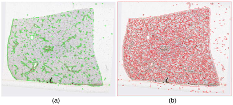
We have tested our method on 54 registered whole slide images of sequential liver tissue sections from one human patient, with z-resolution of 50μm. These biopsy sections are stained by Immunohistochemistry (IHC). The resulting images for analysis are down-sampled from the base level by 64:1, with the final resolution of 1530 × 1373 pixels. We apply our segmentation method to images with parameters: σ₁ = 1, σ₂ = 4, σ₃ = 1.5, λ₁ = λ₂ = 1, α = 65, β = 2, γ = 5. In general, we can have similar results with reasonable perturbations to this parameter set. The segmentation time cost for each image is 43.65 ± 0.63 seconds in Matlab R2013 with Dual Xeon E5420 CPUs at 2.5Ghz. In Fig. 1, we present vessel segmentation results from a typical image where the detected vessels are marked in green. The final vessel detection results in Fig. 1(e) are produced by combining final vessel wall results in Fig. 2(a) with detected lumens after removing candidates with unduly long perimeter length. To further examine the efficacy of VDFE directing level set function to vessel boundaries, we illustrate in Fig. 2 vessel wall segmentation results with and without prior information on vessel wall probability before post-processing. It is apparent that VDFE in Fig. 1(a) navigates zero level set to specific vessel edges in a target segmentation process. By contrast, results without VDFE guidance in Fig. 1(b) show that zero level set partitions the image purely based on fitting error (or homogeneity), with poor selective specificity to primary vessel boundaries. We compare our segmentation results with primary vessel annotations by human. Due to the large number of vessels in presence and variable confidence of vessel recognition by their appearances, only representative primary vessels with high recognition confidence and relatively large size are annotated by human. Table 1 presents the validation results of all one-to-one human-machine vessel pairs measured by Jaccard coefficient, precision, recall, F₁ score, and Hausdorff distance. We also compare our Vessel Directed Level Set (VDLS) method with morphological reconstruction (MR) approach [12] in Table 1. Note that 1336 human-VDLS and 881 human-MR one-to-one vessel pairs from 54 images are found and assessed.

Fig 2.

Primary vessel wall segmentation result of (a) directed and (b) non-directed prior information on vessel wall probability before post-processing.

Table 1.

Evaluation of the segmentation results (Mean ± Standard Deviation).

	Jac	Pre	Rec	F1	H aus
MR	0.45 ± 0.21	0.60 ± 0.27	0.77 ± 0.26	0.59 ± 0.22	34.48 ±75.45
VDLS (our method)	0.84 ± 0.10	0.96 ± 0.06	0.87 ± 0.08	0.91 ± 0.07	6.82 ± 30.99

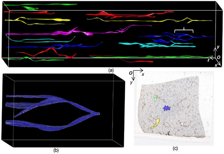
To avoid unduly high vessel association complexity and error, we apply our vessel association approach to top 30 candidates by size on each slide. The most expensive computation is linear programming (64.56 ± 3.49 seconds). The parameters are empirically set as μ₁ = 0.63, ${\kappa }_1^2=50000,{\kappa }_2^2=50$, ω₁ = 0.54, ω₂ = 0.36, κ² = 500, $L_{\mathit{\text{const}}}^{\alpha }=0.5$ and $L_{\mathit{\text{const}}}^{\beta }=0.5$. After vessel association, we perform B-Spline interpolation between adjacent associated vessel objects due to low z-axis data resolution, and volumetrically render the 3D vessel structures. In Fig. 3(a), we present a panoramic view of our 3D visualization result for representative primary vessels from our dataset. One close-up view of a vessel segment is illustrated in Fig. 3(b). The right most image frame observed from right to left in the panoramic view is shown in Fig. 3(c), with color-coded 2D vessel candidates for 3D reconstruction. Note that reconstructed vessels with candidates by MR method are generally shorter due to imperfect vessel identification in intermediate image frames. As our analysis focuses on primary vessels, the vessel association result is relatively robust to registration outputs.

Fig 3.

(a) Panoramic view of 3D reconstructed vessels; (b) a close-up view of a vessel segment indicated by a curly bracket in the panoramic view; (c) color coded vessel candidates in the right most image frame observed from right to left in (a).

4 Conclusion

In this paper, we present an automated framework for 3D primary vessel structure analysis on whole slide histological images of liver tissue sections. For vessel segmentation, we propose an improved variational level set framework with prior information on vessel wall probability. We achieve optimal vessel associations by local bi-slide vessel mapping and global vessel structure association within a MAP framework. Experiments with a real world use case and preliminary evaluations present promising results. In future work, we will assess our method with other larger datasets and extend it to enable micro-vessel analysis.

References

- 1.Foran DJ, Chen W, Yang L. Automated Image Interpretation Computer-assisted Diagnosis. Ana Cell Path. 2011;34(6):279–300. doi: 10.3233/ACP-2011-0046. [DOI] [PMC free article] [PubMed] [Google Scholar]
- 2.Roberts N, Magee D, Song Y, Brabazon K, Shires M, Crellin D, Orsi NM, Quirke R, Quirke P, Treanor D. Toward Routine Use of 3D Histopathology as a Research Tool. Am J of Path. 2012;180(5):1835–1842. doi: 10.1016/j.ajpath.2012.01.033. [DOI] [PMC free article] [PubMed] [Google Scholar]
- 3.Schwier M, Hahn HK, Dahmen U, Dirsch O. Reconstruction of Vessel Structures from Serial Whole Slide Sections of Murine Liver Samples; Proc. SPIE 8676, Medical Imaging; 2013. [Google Scholar]
- 4.Li C, Huang R, Ding Z, Gatenby C, Metaxas D, Gore J. A Level Set Method for Image Segmentation in the Presence of Intensity Inhomogeneity With Application to MRI. IEEE Trans Image Process. 2011;20:2007–2016. doi: 10.1109/TIP.2011.2146190. [DOI] [PMC free article] [PubMed] [Google Scholar]
- 5.Li C, Kao C, Gore JC, Ding Z. Implicit Active Contours Driven by Local Binary Fitting Energy. IEEE Comp Vis and Pat Rec. 2007:1–7. [Google Scholar]
- 6.Frangi AF, Niessen WJ, Vincken KL, Viergever MA. Multiscale Vessel Enhancement Filtering. MICCAI. 1998;1496:130–137. [Google Scholar]
- 7.Ruifrok AC, Johnston DA. Quantification of Histochemical Staining by Color Deconvolution. Anal Quant Cytol Histol. 2001;23:291–299. [PubMed] [Google Scholar]
- 8.Li C, Xu C, Gui C, Fox MD. Distance Regularized Level Set Evolution and Its Application to Image Segmentation. IEEE TIP. 2010;19:3243–3254. doi: 10.1109/TIP.2010.2069690. [DOI] [PubMed] [Google Scholar]
- 9.Dantzig GB. Linear Programming and Extensions. Princeton Press; 1963. [Google Scholar]
- 10.Berclaz J, Fleuret F, Fua P. Multiple Object Tracking using Flow Linear Programming. Winter-PETS; 2009. [Google Scholar]
- 11.Bise R, Yin Z, Kanade T. Reliable Cell Tracking by Global Data Association. ISBI. 2011 [Google Scholar]
- 12.Vincent L. Morphological Grayscale Reconstruction in Image Analysis: Applications and Efficient Algorithms. IEEE TIP. 1993;2:176–201. doi: 10.1109/83.217222. [DOI] [PubMed] [Google Scholar]