Synthesis of a high resolution social contact network for Delhi with application to pandemic planning

Abstract

Objective

We aim to understand quantitatively how targeted-layered containment (TLC) strategies contain an influenza pandemic in a populous urban area such as Delhi, India using networked epidemiology.

Methods

A key contribution of our work is a methodology for the synthesis of a realistic individual-based social contact network for Delhi using a wide variety of open source and commercial data. New techniques were developed to infer daily activities for individuals using aggregate data published in transportation science literature in combination with human development surveys and targeted local surveys. The resulting social contact network is the first such network constructed for any urban region of India. This time varying, spatially explicit network has over 13 million people and more than 200 million people-people contacts. The network has several interesting similarities and differences when compared with similar networks of US cities. Additionally, we use a high performance agent-based modeling environment to study how an influenza-like illness would spread over Delhi. We also analyze well understood pharmaceutical and non-pharmaceutical containment strategies, or a combination thereof (also known as TLCs), to control a pandemic outbreak.

Results

(i) TLC strategies produce the mildest and most delayed epidemic out-break than any of the individual interventions; (ii) the epidemic dynamics of Delhi appear to be strongly influenced by the activity patterns and the demographic structure of its local residents; and (iii) a high resolution social contact network helps in analyzing effective public health policies.

Conclusion

A high resolution synthetic network is constructed based on surveyed data. It captures the underlying contact structure of a certain population and can be used to quantitatively analyze public health policy effectiveness. To the best of our knowledge, this study is the first of its kind in the Indian sub-continent.

1. Introduction

Today's densely populated urban regions facilitate a swift transmission of infectious airborne diseases [1]. Additionally, urban contact networks in regions like India and China are witnessing rapid growth. Delhi, officially recognized as the National Capital Territory (NCT) of India, is predicted to rise in population from 16.7 million in 2011 to 22.5 million in 2021 primarily due to a high rate of in-migration [2]. In Beijing, the population rose from 12.9 million in 2000 to 18.8 million in 2010 [3]. The ever increasing density of these urban regions can further increase the risk of an unmitigated pandemic. Consequently, public health authorities around the world have focused on developing effective policies to control the spread of diseases. The close coordination among the authorities, use of data driven computational models, and timely interventions have helped in controlling a number of recent outbreaks. Pharmaceutical as well as social distancing based interventions have proved themselves effective in this regard.

An epidemic diffuses through both dimensions of space and time [4]. Work on travel and mobility analysis [5–8] has prepared us for better observations in this regard. Networked computational epidemiology is the use of computer models to understand the spatio-temporal diffusion of disease through populations using a synthetic yet realistic representation of the underlying social contact network [9]. The basic approach is now widely accepted in the epidemiology community [10–12]. Researchers agree that a better understanding of social contact network characteristics can provide novel insights into the disease dynamics and intervention strategies for effective epidemic planning.

A methodology to synthesize realistic social contact networks already exists for United States cities. Contact networks for United States cities are generated by following a 3-step process. (i) A baseline population is synthesized based on sociodemographic statistics and microsample data from the United States Census. (ii) Mobility patterns from a nationwide household survey and land use data in the form of work, retail, recreational, school, and college locations are used to infer the spatio-temporal mobility patterns of individuals. (iii) User specified interaction criteria is used to estimate region-specific contact networks. The structure of the resulting social networks, calibrated to the above data, has been shown to influence the outcome of disease outbreaks in our simulated epidemic models [9, 13].

Since the synthetic network should provide a realistic representation of the contact network specific to that region, the process to generate the contact network utilizes region-specific data. The United States synthetic population captures details of household structure by utilizing the 5% Public Use Microdata Sample for each Public Use Microdata Area that is modeled. The United States National Household Travel Survey (NHTS) [14] captures the interdependence of people's activities in the same household across all surveyed households in the United States. Data with a similar degree of detail is not available for many other regions (including Delhi, India), making it impossible to replicate the United States network generation process for regions outside the United States.

1.1. Summary of contributions

Building on our earlier work, we construct a synthetic social contact network for Delhi. To overcome data limitations for Delhi, we developed several new methods, many of which are generic enough to be easily applied to the synthesis of networks for urban regions in other developing countries. To the best of our knowledge, this is the first such synthetic representation of a contact network for an urban region in South Asia. Using a variety of data sources, a synthetic contact structure with detailed demographic information for each person, a minute-by-minute schedule of their activities, and the locations where these activities take place is generated by a combination of simulation and data fusion techniques. This yields a dynamic social contact network represented by a labeled bipartite graph G_PL, where P is the set of synthetic individuals and L is the set of locations. If a person p ∈ P visits a location ℓ ∈ L, there is an edge (p, ℓ, label) between them, where label here is a record of the type of activity of the visit and its start and end times. The synthetic social contact network is: (i) spatially explicit – home locations, work locations, business locations, educational institutions, government institutions, and other places of interest are explicitly represented; (ii) time varying – individuals carry out daily activities for a normative day by potentially visiting several locations, and in turn interacting with other individuals visiting the same locations during the same time period, and (iii) labeled – both individuals and locations carry a range of attributes described in the subsequent sections. Note that it is impossible to build such a network by simply collecting field data. The use of generative models to build such networks is a unique feature of this work.

We then use high-performance agent-based simulations to study the spread of an influenza-like illness over the synthetic social contact network of Delhi. We study the efficacy of various intervention strategies, including pharmaceutical and non-pharmaceutical interventions. We rank these strategies by order of their efficacy and discuss how the outcome of the simulated intervention experiments compares with those reported for other cities in the world. Finally, we carry out a detailed sensitivity analysis to assess the robustness of our conclusions.

1.2. Significance

The methodology and results presented in this paper extend our earlier work in a number of ways. First, we employ novel data sources and data integration methods. The methods we developed to synthesize urban scale social contact networks were based on data sources that were easily available. Many of these data sources are not easy to obtain for other countries. For example, the way we model people's activity sequences based on aggregated statistics is new. Furthermore, the basic method is generic and thus is applicable in other countries with similar limitations. Second, our work yields the first synthetic social contact network for Delhi. Very few if any such networks have been synthesized for urban areas in developing countries. Although the focus of the present paper is public health epidemiology, the social contact network synthesized can be used in a number of other applications; e.g. evacuation planning or urban transportation planning [15]. New methods are also presented to analyze massive social contact networks. For example, graphlets describing the demographic structure of people-people contacts are employed to analyze people's interaction patterns – recently these methods were used in the context of analyzing mobility patterns [16, 17]. Finally, our results confirm that a targeted layer containment (TLC) strategy is effective in controlling an influenza epidemic in Delhi. TLC strategies have been proposed and extensively analyzed in [18]. As expected, vaccinations are effective, but their effectiveness depends on compliance and vaccine efficacy. Influenza vaccines continue to yield mixed results as has been discussed in epidemiology literature. Thus TLC as a combination of social distancing and pharmaceutical interventions can be seen as a natural and implementable alternative.

The remainder of the paper is organized as follows. Section 2 presents the new methodology to generate the detailed network and an overview of the data used for this methodology. In Section 3, we analyze structural properties of this network and compare effectiveness of different public health interventions in the H1N1 epidemic in Delhi using simulations. We assess the robustness of our epidemiological findings to synthesized social contact network. This is further discussed in Section 4.1. Section 4.2 contains a detailed discussion of graph structural properties of the resulting network and their comparisons with those of the coarse network. Section 4.3 summarizes our efforts in validating the synthesized networks. Finally, section 5 concludes with remarks on future research.

1.3. Related work

Traditionally, mathematical and computational modeling of epidemics has focused on aggregate models using coupled rate equations [19]. In this approach, a population is divided into compartments according to an individual's health state (e.g., susceptible, exposed, infected, or recovered) and his/her demographic group. The evolution of the infectious disease is then characterized by ordinary differential equations. For analytical tractability, these models assume homogeneous mixing, which limits their use for spatially sensitive processes.

In recent years, high-resolution individual-based computational models have been developed to support the planning, control, and response to epidemics. These models support networked epidemiology, that is the study of epidemic processes over explicit social contact networks. Research in this area can be divided into three distinct subareas.

Work in the first subarea aims to develop analytical techniques and computer simulations over classes of progressively sophisticated random graphs [20, 21]. These models relax the mean field assumption to some extent, but still use the inherent symmetries in random graphs to analytically compute important epidemic quantities of interest. The primary goal of these techniques is to obtain closed form analytical results.

The second subarea aims to develop individual-based models using important statistics associated with a given region. Two important statistics that are often used are: (i) population density — it is usually obtained using LandScan data, and (ii) the demographic distribution of individuals within a population that is typically obtained from the region's census. A simple template is used to represent subcommunities (for example, counties) and these subcommunities are joined hierarchically to obtain larger regions. See [22–26] for examples of this approach. These models can be combined to obtain hybrid models where, for instance, counties may be represented as nodes and edges are added between counties to capture the movement of individuals (see [27–29] for a comparative study). Epidemic dynamics within a county can then be computed using an individual-based model. The epidemic dynamics between counties are captured using coupled rate equations.

The final class of models use the most realistic representation of social contact networks; see [30–32]. In [31–34] each individual in the United States is modeled with a detailed demographic profile and a daily activity-location schedule. Our synthetic social network for Delhi is constructed using this class of models.

2. Data and methodology

In this section, we describe our methodology for constructing a high resolution social contact network for Delhi. The methodology builds on our previous work in the context of US cities [13, 35]. As mentioned earlier, a significant challenge faced when synthesizing networks for developing countries is lack of readily available data. We use a number of imputation techniques to overcome this challenge.

2.1. Data collection

Delhi in the paper refers to the NCT of India, including New Delhi and the adjacent urban areas in the neighboring states. We model the population of Delhi based on the India Census of 2001 – it was the most recent census when we began this work. Delhi contained over 13 million people in 2001 and is one of the regions with the highest population density in the world. The average population age is fairly young with a high male to female ratio. Important population statistics are summarized in Table 1; and are compared with other representative cities in the world.

Table 1. Demographic statistics of Delhi in comparison with two other cities.

City	Population size	Average age	Average household size	Sex ratio (M/F)
Beijing	16.20M	37.9	2.6	0.99
Delhi	13.85M	25.6	5.14	1.22
Los Angeles	16.23M	32.9	3.0	0.97

Multiple sources of data are required for constructing a contact network, including demographics, activity patterns and land use information about the region. The data we collected and used to construct the Delhi network is listed in Table 2.

Table 2.

The demographics, location, and activity data used in the construction of the Delhi network.

	Data set	Description
Demographics	India Census 2001 [36]	Statistics for demographic variables such as age, gender, income, etc. at the individual level and household level for Delhi residents.
	Household microdata: India human development survey 2005, conducted by the University of Maryland and the National Council of Applied Economic Research (IHDS2005) [37]	The data has micro samples for household (HH) structure, and comes from 960 households in Delhi, including 4620 individuals. It describes for each HH sample: HH size, householder's age, HH income, house types, animal care; it also depicts each individual in the HH: demographic details, religion, work, marital status, relationship to the householder, etc.
Locations	MapMyIndia map dataset [38]	It includes the following information for Delhi: (1) ward-wise statistics for population and households in 2001; (2) coordinates for locations such as residential areas, schools, shopping centers, hotels; (3) infrastructures such as roads, railway stations, land use; (4) boundary for each city, town and ward.
Activity	Thane India 2001 travel survey by University of South Florida [39]	The raw survey data was unavailable. However, literature on the survey reports statistics on the socio-demographics, profile of the survey participants, their trip frequency distribution, and their trip start time, and duration distribution.
	2000 to 2007 school attendance statistics from UNICEF [40]	School attendance rates among school age children in India.
	India residential area activity survey by the Network Dynamics and Simulation Science Laboratory (NDSSL) at Virginia Tech	The survey focuses on the approximately 40% of adults in India who do not travel to work. Participants' age, gender, and contact duration near their home are collected.

2.2. Network construction methodology

The procedure to construct the Delhi network follows three key steps: (i) synthesis of a baseline population with detailed individual structure that is statistically consistent with the true population; (ii) assignment of a reasonable activity schedule to each individual; and (iii) assignment of locations for activities of each synthetic individual. Section 2.2.2 and 2.2.4 introduce new methodology for performing step (ii) and a part of step (iii) that assigns residential locations to individuals. The remainder of the synthesis process follows largely from our approach in [35] and are calibrated to new and alternative data summarized in Table 2.

2.2.1. Synthetic population generation with the India Census of 2001 and micro household sample data

A synthetic population is a set of synthetic people, each associated with demographic variables drawn from any of the demographic distributions in the census or similar aggregate data sources. Joint demographic distributions can be reconstructed from the marginal distributions using an iterative proportional fitting (IPF) technique. Each synthetic individual is placed in a household with other synthetic people and each household is located geographically in such a way that a census of our synthetic population yields results that are statistically indistinguishable from the original census data, if they are both aggregated to the same geographical level. Synthetic populations are thus statistically indistinguishable from the census or any other aggregate data used; nevertheless since they are synthetic they respect the privacy of individuals that they were designed to represent. Note that, census tables are precisely constructed so as to respect privacy: our methods are a way to disaggregate these tables in a statistically sound manner. The synthetic individuals carry with them a complete range of demographic attributes, such as income level, age, etc., collected from the census data.

In doing this, our method makes use of the summary statistics of what we deem as relevant demographic variables at household level (India Census 2001 [36]) and a collection of household samples from India human development survey 2005 by University of Maryland (IHDS2005 [37]). Household samples in IHDS2005 come from 960 households in Delhi, comprising of 4620 individuals. They describe demographic attributes of each household sample and each individual in the household, as listed in Table 2. This is our first example of data imputation. Public use microdata (PUMS) is usually available for cities in the US but is currently not available for India. Nevertheless, IHDS2005 survey is extensive and provides this information. The data had to be reformatted to produce a PUMS-like sample for the Delhi region. A flowchart of the method is illustrated in Figure 1. The synthesized population with realistic household structures is illustrated in Figure 2. Delhi is divided into 114 wards (an administrative region); a synthetic subpopulation is created for each ward separately using the above algorithm.

Figure 1.

Flow chart for synthetic population generation: create synthetic households by sampling from the joint distribution of demographic variables, in conjunction with household micro-samples. The parallelograms represent data sets and the rectangles represent algorithms used in processing data. The algorithm IPF is used to estimate the joint distribution table of demographic variables.

Figure 2.

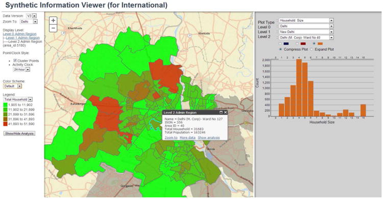
Our laboratory has developed an interactive web-based graphical tool called Synthetic Information Viewer to visualize the synthesized population. The figure shows a map of Delhi and its 114 wards. For example, clicking on ward No. 40 shows the statistics of synthetic households in the ward, which comprise of 31,683 households and 163,246 individuals. The right panel displays the household size distribution for the synthetic households in ward No. 40.

2.2.2. Activity assignment using the 2001 Thane, India household travel survey statistics

If available, raw travel survey data for Delhi would have afforded a direct implementation of the activity assignment method described in [35] as the next step toward building the Delhi synthetic network. Such data was not easily accessible at the time of this study. However, due to the availability of detailed summary statistics of the 2001 Thane, India travel survey in literature [39, 41], we devise a discrete-time simulation to generate and assign activity schedules to the Delhi synthetic population. Thane is a city in the western state of Maharashtra, India. A quick comparison of census statistics between Delhi and Thane [36] reveals a high degree of similarity in the demographic structure and their religious/cultural habits. As a result, we consider Thane to be a reasonable proxy for Delhi, as far as activity modeling is concerned.

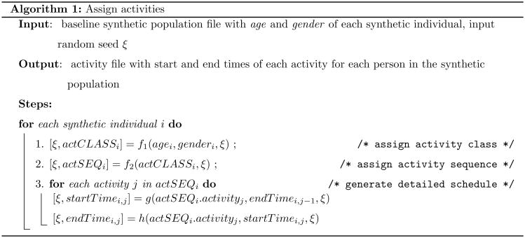
The 2001 Thane household travel survey is a trip-based survey that collected travel data in the form of 24-hour trip diaries from 14,428 respondents in 3,505 households in the metropolitan region of Thane. Additionally, the survey collected sociodemographic information from respondents and their respective households. Literature on the Thane travel survey describes the sociodemographic profile of mobile adults (adults that recorded at least one trip) and people recording no trips, as well as travel data statistics in the form of distributions of trip start times and trip durations of the survey sample population. Personal and household trip rates are reported as a function of mode of transportation, household size, and individual worker status. The literature also briefly describes trip frequency, activity characteristics, and time use characteristics of students younger than 16 years old, students older than 15 years old, and mobile adults. Detailed trip chaining analysis is also reported for commuters (adults reporting at least one work-based trip). All trips reported in the survey began at home and ended at home. Based on the Thane survey statistics reported in [39] and [41], the activity assignment process described in Algorithm 1 generates a sequence of activities, along with their start and end times, for a normative 24-hour day for each synthetic person in the population. Each set of activity assignments for a synthetic person are independent of the activity assignments to people from other households in the synthetic population.

For each person in the baseline population, the algorithm first assigns an activity class depending on his/her demographics (namely, age and gender). For adults, this is achieved by sampling from the commuter status and demographic distribution of adults in the survey population reported in [41]. The algorithm classifies synthetic adults as commuters (adults reporting at least one work related trip), non-commuters (mobile adults with no work related trips), or zero trip makers. We further assume all adult non-commuters between the age of 18 and 23 have school related activities and classify them as college attendees. Since the literature reports commuter status statistics only for adults, we make the following assumptions about individuals aged 17 years or less, henceforth referred to as children. Children 6 to 10 years old are classified as primary school attendees, non-school goers making at least one trip in a day, or zero trip makers. Similarly, children 11 to 17 years old are classified as secondary school attendees, non-school goers that make at least one trip in a day, or zero trip makers. These assumptions are made based on observations from the real world. The distribution of primary and secondary school attendees, non-school going children and children with no trips in the synthetic population is set to match the net enrollment ratios of primary and secondary schools all over India from 2000 to 2007 [40] as well as the fraction of zero trip makers in the age range 6 through 17 years in the Thane sample. The activity class assignment for both children and adults is represented by function f₁ in step 1 of the algorithm.

In step 2, the activity class of the synthetic individual is used to decide his/her activity sequence by sampling from an empirical frequency distribution of reported activity sequences in the Thane survey. The Thane survey describes each recorded trip by the origin and destination of the trip, namely, home, work, shop, school (or college), social/recreational, and all other location categories. These six location types along with “travel” define the seven distinct activities that constitute an activity sequence. Individuals classified as zero trip makers are assigned a home activity for all 24 hours of the day. More than 99% of the students in the Thane survey report exactly two trips in a day [41]: home to school and school to home. As a result, we assign the activity sequence home – travel – school (college) – travel – home to all school or college attendees. The algorithm defines all non-working adults and non-school going individuals reporting at least one trip during the day and with no school or work related activities as non-commuters. Nearly all non-commuting adults report exactly two trips in a day [41], of which approximately half reported the activity sequence: home – travel – shop – travel – home, a quarter reported the activity sequence: home – travel – social/recreational – travel – home, and the remainder reported the sequence: home – travel – other – travel – home. Since available literature provides no information on non-commuter children in the survey, we assume that the above frequency distribution of activity sequences of non-commuting adults applies to non-commuter children as well. Commuters report eight distinct activity sequences, of which 97.34% report only two trips in a day: home to work and work to home. The activity sequence assignment process for both children and adults is represented by function f₂ in step 2 of the algorithm.

Finally, in step 3 of the algorithm, a detailed activity schedule with start and end times for each activity in the sequence is generated by sampling from reported empirical frequency distributions of trip start times and trip durations. For each activity in the activity sequence, the algorithm samples from the relevant trip start time and trip duration empirical distributions (represented by functions g and h, respectively, in the algorithm) conditional on the time left until the end of the day. Since the literature does not report start time and the trip duration distributions for school or college related trips, we assign a fixed schedule to all primary school, secondary school and college attending individuals.

2.2.3. Location creation, assignment and contact network estimation

Locations are where people conduct their activities (including household activities). They decide how people are distributed in the geographical space of the city. The data set of MapMyIndia [38] contains land use statistics for Delhi, including geo-coordinates for various classes of points of interest (POI). This includes, work locations, malls and shopping centers, recreational places, office buildings, etc. MapMyIndia provides one of the most extensive POIs for Indian cities. Although the data was collected for mapping services, it provides just the kind of information we need. We extracted coordinates for these POIs and assigned people to those locations for their daytime activities. Schools, colleges, shopping centers and other places are also considered as work places. For example, schools are places students take classes, but they are also work places for teachers.

Home locations are possibly the most important of all location as they represent the place where individuals spend the most time. We do not have a complete data set for real home coordinates. However, the city of Delhi is divided into 114 wards and we know the number of households in each ward (Figure 2), which helps us correctly (at the ward level) distribute home addresses over the whole city.

After we assign people to locations based on their activities, we then capture their geo-spatial positions over the course of a day. In Figure 3 we illustrate such travel routes for three members in a typical family.

Figure 3.

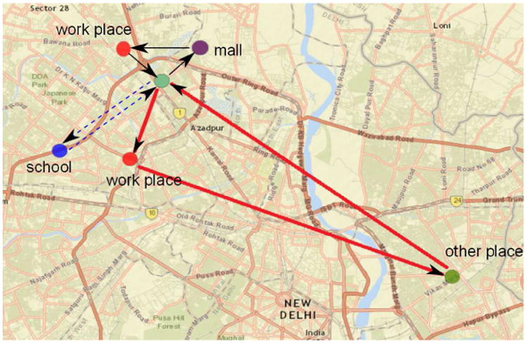
The daily travel routes for all three members in a family. The routes for different members use different line style. Father's routes are shown as solid thick lines: home→work place→other place→home; mother's are solid thin lines: home→mall→work place→home; son's are dash lines: home→school→home.

Once we know the subgroup of people who visit each location, A people-location bipartite graph G_PL can be inferred. Here P is the set of people and L is the set of locations. If a person p ∈ P visits a location ℓ ∈ L, there is an edge (p, ℓ, label) ∈ E(G_PL) between them, where label is a record of the type of activity and its start and end time.

A people-people contact network G_P can be inferred from G_PL. Potential people-people contacts occur when two persons coexist in the same location at the same time. If a location is large, however, two people may not meet even if they are there simultaneously. Therefore, we measure people-people interactions within a location via its sublocation structure. For example, a sublocation could be a room in a building, and people in a room at the same time are considered to be in contact with each other.

For each location type, we select an empirical number as the sublocation size. The sublocation size is an important parameter characterizing the interactions of people within a location. We will discuss potential errors due to a biased sublocation sizing in section 4.1.

2.2.4. Contacts in residential area

As a characteristic social-economic phenomenon in India, about 40% of the population do not travel on a daily basis and stay around their residential areas for the entire day. This observation is verified by two independent sources, a nationwide household survey conducted for India [37], and the Thane travel survey we retrieved from [39]. We believe that this is an important socio-cultural difference between developed nations such as the US, and developing nations such as India, that can critically impact contagions.

This motivates us to carefully model the interactions among those people who stay home as their percentage is far from being negligible. We conducted a survey in Delhi and several other nearby cities, collecting data on “at-home people” within a residential area (Table 2). Since these people reported no travel on a daily basis, we assume they are in contact only with people within their own locality. The survey gives us the typical number and duration of contacts for people in different demographic groups, and who they are in contact with. The data suggests that residential contacts tend to be volatile and mix homogeneously within similarly aged people. We further assume that these contacts are highly clustered like any typical social network. With this information, we model contacts between people in residential areas as follows. First, we extract probabilistic distributions of contact number and contact duration for each age/gender group from the survey. Second, given each person's age and gender, we sample his/her degree from the contact number distribution. Consequently, we get a degree list for all the people in a residential area. Third, given the degree list, we use a configuration model with the added feature of preserving triads [42] to generate a random network. The edge weights are calibrated using the contact duration distribution. We call the generated network a residential network, and edges in the network are deemed residential contacts.

We repeat the above process for each residential area in the city to get a set of residential networks. We then incorporate these residential networks into the Delhi network by simply putting all the edges in the residential networks into the Delhi network.

2.3. Simulation scenarios

We run epidemic simulations on the Delhi contact network to understand the epidemic dynamics and the effects of public health policies in the Delhi population. To fulfill this requirement, we simulate the spread of H1N1 [43] in our experiments. The implementation details are shown in the following.

2.3.1. Epidemic model

The disease progression in the individual-based model follows the standard susceptible-exposed-infectious-recovered (SEIR) model. Details of the disease transmission models, which characterize both within-host disease progression and between-host disease propagation, can be found in the appendix of [44]. Three key parameters to the epidemic dynamics are the basic reproduction number, R₀; the incubation period distribution and the infectious period distribution. (i) R₀ is the number of secondary cases one case generates on average in a previously unaffected population. The R₀ of H1N1 has been studied extensively: 1.45 is estimated for India [45], estimations in other regions range from 1.20 to 1.68 [46–50]. The aforementioned values are only estimates, no unique “precise” value is agreed upon. To address the variations in different estimates for R₀ of H1N1 in the literature, we choose a set of values: 1.35, 1.40, 1.45, and 1.60. The range of these values covers most estimates found in the literature. (ii) The incubation period is the interval between exposure to an infectious disease and the appearance of the first signs or symptoms, and usually lasts 1-4 days for seasonal influenza [51]. (iii) The infectious period is the interval during which infected individuals can spread the disease to susceptible individuals. The period typically lasts 3-5 days [51]. The incubation and infectious periods in our model are described using discrete probability distributions since their actual lengths vary for different individuals. In the experiments, we select the discrete distribution for the incubation period as “1:0.3 2:0.5 3:0.2”, meaning that an exposed individual stays in incubation status for 1 day with a probability 0.3, 2 days with a probability 0.5 and 3 days 0.2. Similarly, we select the distribution for the infectious period as “3:0.3 4:0.4 5:0.2 6:0.1”. We therefore design four different disease models, each differing from the others only in its R₀ value (we use the same distributions of incubation and infectious periods in all models).

2.3.2. Intervention strategies

Informally, an intervention changes one or more attributes of a set of individuals. Some of the attributes correspond to behavioral changes, such as home isolation, use of a face mask, cutting down non-essential activities, etc. Other attributes correspond to disease specific changes such as immunity of an individual to a disease, level of infectiousness, infectious period duration, etc. The first type of interventions change the social contact network by adding or deleting edges, or modifying the edge labels (usually contact durations). The second type of interventions change the vertex properties directly. Interventions are either a result of public health policies, in which a group of individuals are simultaneously affected, or based on the perception of the disease by individuals or by households. From an abstract standpoint, an intervention changes the label of a subset of vertices or edges of the contact network.

We simulate four public health policies frequently applied in the real world, including pharmaceutical interventions (PI) and non-pharmaceutical interventions (NPI). PI includes antiviral and vaccination; NPI includes school closure and work closure. The two PIs are the second type of interventions that change the vertex properties; and the two NPIs are the first type of interventions. Each intervention contains three components: the subpopulation to which we apply the interventions; the triggering condition; and the action taken. The details of the four interventions regarding the three components can be found in Table 3.

Table 3. Intervention implementations.

Intervention	Subpopulation	Triggering condition	Action
antiviral	randomly selected 25% population	over 0.1% population are infected	reduce infectivity
vaccination	randomly selected 25% population	over 0.1% population are infected	increase their immunity
school closure	apply to students with 60% compliance	over 0.1% population are infected	remove in-school contacts between them
work closure	apply to workers with 60% compliance	over 0.1% population are infected	remove work contacts between them

2.3.3. Targeted-layered containment

In practice, a combination of multiple interventions are often applied, which includes targeted interventions to specific people as well as general interventions. Such a combination of various interventions is called targeted-layered containment (TLC) [18]. We consider the four specific TLC policies (see list below), and examine multiple levels of compliance with the interventions and infection rate thresholds for triggering the interventions. Vaccination is excluded, since it was not available at the early stage of the 2009 H1N1 epidemics.

• Targeted antiviral: diagnosed individuals are applied antiviral treatment (under some compliance).

• Targeted stay-home: diagnosed individuals are suggested to stay at home (under some compliance).

• School closure: students' school activities are removed (under some compliance and initiated with specific infection-rate threshold).

• Work closure: work places are closed (under some compliance and initiated with specific infection-rate threshold).

3. Results

We generate the Delhi network (both G_PL and G_P) using the data listed in Table 2 and the methodology outlined in Section 2. In the following, we conduct a detailed analysis of the synthetic Delhi population and network. We then use EpiFast [34], a fast epidemic simulation platform, to study the effect of various intervention strategies on the spread of influenza-like diseases in Delhi.

EpiFast is an MPI-based parallel code. We used it to run our epidemic simulations on a cluster comprising of 96 multiprocessor compute nodes. Each node contains 2 Intel Quad-Core Xeon E5440 processors with 3.0GHz, and 16 GB of memory. The cluster operates SUSE Linux Enterprise Server 10.2. Each simulation in this section makes use of only 12 nodes and the running time ranges from 10 to 20 minutes.

3.1. Demographics and daily activity pattern of the synthetic population

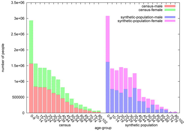
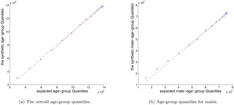
In Figure 4, we compare the individual level demographics of the synthetic population and the true population of Delhi. The linearity of points in the Q-Q plot in Figure 6a suggests that the age distribution of the synthetic population matches that of the true population. However, there is a deviation of the age distribution of males (and consequently, of females) in the synthetic population from that of the reported distribution of males (and of females) in the census (Figure 6b), especially among the younger age groups. The deviation is due to the micro household samples while generating the households, but is relatively small and can be neglected for the purpose of our study.

Figure 4.

The graph on the left depicts the age-group counts for Delhi from the India Census 2001 [36]. The one on the right depicts the age-group counts of the synthetic population. The synthetic population appears to conform to the census statistics. The QQ-plots in Figure 6 relate the similarities in a more precise sense.

Figure 6.

Q-Q plots of the age-group quantiles for the synthetic Delhi population. In Figure 6a, the age-group quantiles of the synthetic population conform very well with the expected value based on the census data. A slight but acceptable deviation from 45 degree line is observed in the males only curve (see Figure 6b)

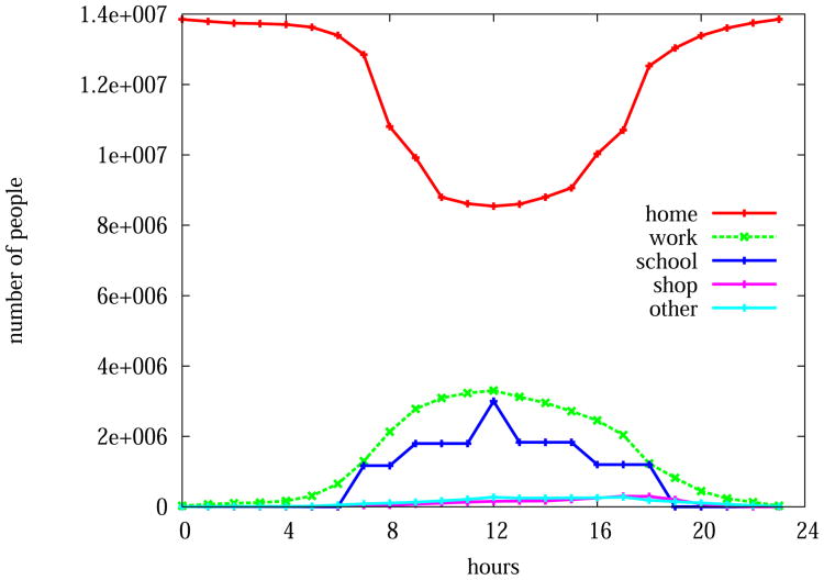
Figure 5 compares the activity statistics for the synthetic population. We calculate for each hour in a typical day the number of people performing a specific type of activities, for example: home, work, school, etc. Of the five major activity types, “home” appears to be dominant. At any given time, there are more people at home than at all other locations. This is due to the special socioeconomic structure in India where about 40% of people do not travel on a daily basis. This 40% comprises of stay-at-home women, the elderly, and a portion of young people. This phenomenon is observed in the Thane survey and is assumed to be true for Delhi as well. Most people work or study during the day, and almost all people stay home at night. This cultural feature is quite different from a typical city in the US.

Figure 5.

The graph shows temporal activity of the synthetic population. Each curve represents the total hourly count of individuals in the synthetic population engaged in a particular type of activities across a 24-hour day. During the late night(hour 0 and 24), almost all people stay at home.

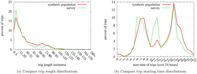
For the Thane travel survey, the travel pattern statistics in terms of trip length distributions and trip starting time distributions are available. To validate Algorithm 1, we compare these two distributions in the synthetic population with that in the survey data. Figure 7a shows the consistency of the trip length distribution between the output data and the input data of Algorithm 1. In Figure 7b, however, the trip starting time distribution seems to be consistent between the synthetic data and the survey data for trips starting in the morning and in the afternoon, but not for those trips starting around noon time. This is due to the fact that these are mostly short lunch break trips, which we ignored for simplification in the activity assignment algorithm. While we argue that such simplification has little impact on the epidemiological outcomes of our experiments in this paper, we plan to improve Algorithm 1 in our future work to remove the discrepancy in the trip starting time distribution.

Figure 7.

The above curves represent the trip length distributions (Figure 7a), and trip starting time distributions (Figure 7b) in the Delhi synthetic population and the survey.

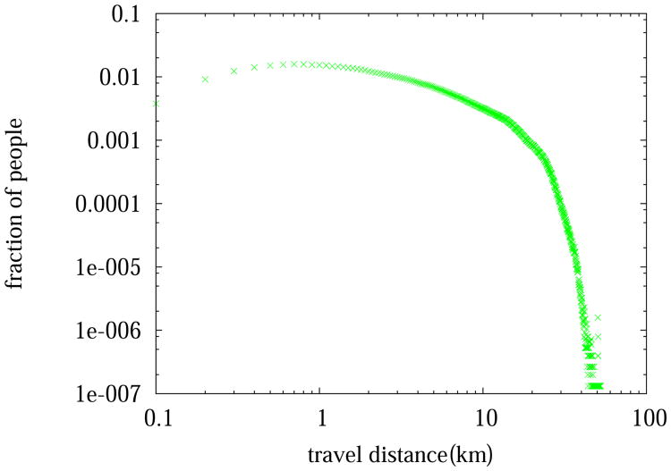
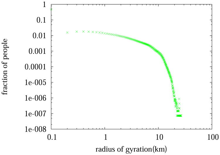
Next, we turn our attention to the mobility metrics for the synthetic population. People's mobility patterns are a key factor to the spread of epidemics. We consider two measures in this regard, the daily travel distance and the radius of gyration. The daily travel distance for an individual is their total travel distance on a typical day. Assume a person visited N places on a day (repetitive visits to the same place are counted as multiple places), then the person's radius of gyration is defined as:

$$R_g=\sqrt{\frac{1}{N}\sum _{k=1}^N{(r_k-r_{\mathit{\text{mean}}})}^2}$$

where r_mean is the mean position of the N visited places, and r_k refers to the position of the kth place. The travel distance measures the amount of movement, while the radius of gyration measures the area covered by a person's movement. From Figures 8 and 9, we observe that the distributions of the two metrics appear to follow a truncated power law curve. This is consistent with the findings in the literature [7].

Figure 8.

The daily travel distance distribution of people in Delhi within a 24-hour-period.

Figure 9.

The radius of gyration distribution of people in Delhi measured over a 24-hour-period.

3.2. Graph structural properties of the contact networks

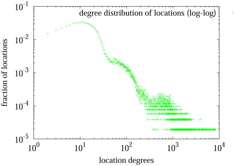
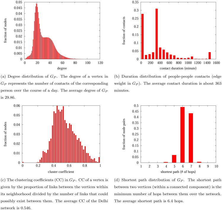
Metrics related to structural analysis of G_PL and G_P are shown in Figures 10 and 11. The bipartite people-location graph G_PL has 13.85 million people and 1.11 million locations. Its degree distribution is plotted in log-log scale in Figure 10. A large part of the degree sequence follows a power law distribution, which appears consistent to findings in other studies [9]. For G_P, we plot the distributions of node degrees, clustering coefficients and contact durations. Naturally, the degree distribution in G_P cannot be compared to that of G_PL. To get a better understanding of their implications on an epidemic, we compare the graph structural properties of the Delhi network against those of the Los Angeles network in Table 4. The degree distribution of the Delhi network G_p peaks around 20. The average degree is about 30, which is relatively small when compared to US cities [52]. Compared to the Los Angeles social contact network, the Delhi social contact network has higher total contact duration and clustering coefficient.

Figure 10.

Degree distribution of locations in the bipartite graph G_PL. A location degree is measured as the number of people that visit the location in a day. Location degrees for the Delhi G_PL range from 1 to 8230 and show a power law like distribution.

Figure 11.

Network structure profiling for the Delhi network (G_P). G_P may contain multiple connected components. The above distributions are computed by aggregating over all its connected components.

Table 4.

Structural properties of two city-scale contact networks.

people-people network	No. of edges	number of nodes	Avg. degree	Avg. edge weight (minute)	Avg. CC
the Delhi network	206,787,386	13,850,507	29.86	363	0.546
the Los Angeles network [52]	459,273,880	16,228,759	56.60	141	0.389

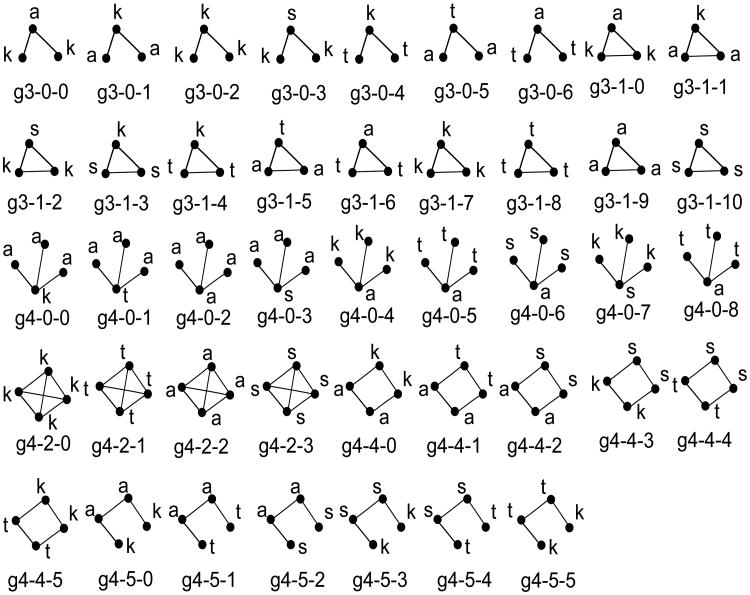
Graphlets are another important feature that have been extensively studied in different applications of network science [7, 53, 54]. G_PL and G_P are relational networks; labels on their edges and nodes capture important demographic and other social features. Here we examine a number of 3-node and 4-node graphlets visualized in Figure 12. Note that all edges are bi-directional and that each graphlet represents an isomorphism class. Two graphs H₁, H₂ are isomorphic if there is a bijection between the vertex sets of H₁, H₂: f: V (H₁) ↦ V (H₂), such that {u, ν} is an edge in H₁ if and only if {f(u), f(ν)} is an edge in H₂; and vertex labels (k, t, a, s) are invariants under the bijection, i.e., u.label=f(u).label.

Figure 12.

Visualization for labeled graphlets, where each graphlet represents an isomorphism class. The node labels k, t, a and s represent preschool children, school students(mostly are teenagers), adults and seniors, respectively. By children we refer to those aged 1 to 5 years, students 6 to 18 years, adults 19 to 60 years, and seniors older than 60 years.

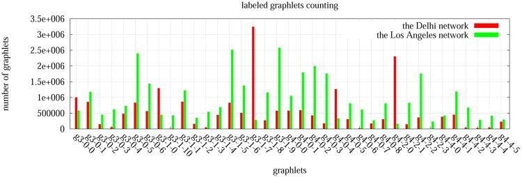
The counts of these featured graphlets in the Delhi network are shown in Figure 13. Additionally, we compare the graphlet distribution to that in the Los Angeles network. A significant structural difference of the two networks is revealed in terms of the graphlet decomposition. From the histogram we can see that Los Angeles peaks at g3-1-9 while Delhi peaks at g3-1-7 and g4-2-0. Since g3-1-9 is an interaction triplet between three adults while g3-1-7 and g4-2-0 represent intensive interactions among three or four children, the different peaks show in a straightforward way that children contribute more in the social interaction activities in Delhi than in Los Angeles. More interesting patterns could be found through further comparisons.

Figure 13.

Distribution of labeled graphlets. See Figure 12 for a visualization of each of the 37 graphlets labeled above.

3.3. Epidemic dynamics and intervention policies

We now turn our attention to disease dynamics over the Delhi network. We focus on influenza-like illnesses and simulate epidemics for a range of R₀ values enumerated in section 2.3.1.

3.3.1. Analysis of node vulnerability

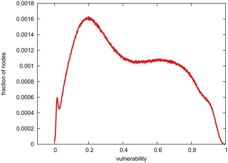
We define vulnerability of a node ν as the probability of ν being infected during an epidemic. We estimate this probability from 10,000 independent random runs of simulation. The distribution of node vulnerability for R₀ = 1.35 is shown in Figure 14. The distributions for other R₀ values are very similar to that of R₀ = 1.35 (and hence omitted in the interest of brevity), indicating that node vulnerability is more relevant to the network structure than to the disease property. This implies that the following observations from the vulnerability distribution are applicable to a multitude of diseases regardless of their R₀.

Figure 14.

The vulnerability distribution of the Delhi network. This is based on 10,000 independent epidemic simulations with R₀ = 1.35. In the figure, the fraction of low vulnerability nodes are more than the fraction of high vulnerability nodes, with about 40% of people having a vulnerability lower than 0.35.

In the case of the Delhi network, the vulnerability distribution of nodes (and thus individuals) is skewed to the right. It appears to have a large mass around 0.2.

3.3.2. Optimal intervention strategies during an epidemic

Next, we study the role of interventions in controlling the epidemics in the Delhi network. To do so, we simulate the four public health policies described in section 2.3.2, including pharmaceutical interventions (antiviral and vaccination) and non-pharmaceutical interventions (school closure and work closure). The simulation results when R₀ = 1.35 are presented in Figure 15. The results when R₀ is 1.40, 1.45 and 1.60 are omitted once again, because they are all very similar to what we observe for R₀ = 1.35. The insensitivity of the simulation outcome to R₀ suggests that the ordering of the policy effects remain unchanged regardless of the R₀ value of a disease.

Figure 15.

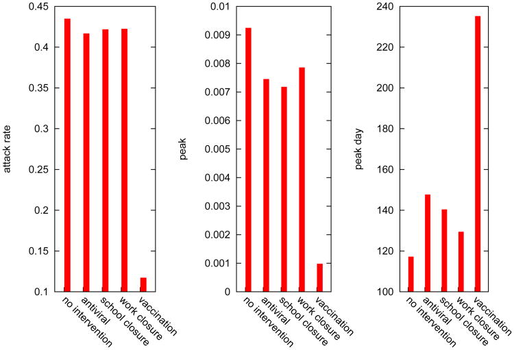
Epidemic simulation outcomes under various intervention strategies on the Delhi network for R₀ = 1.35. The graphs also include a base case where no intervention is conducted. Here we use the 3-tuple (attack-rate, peak, peak-day) to characterize epidemic dynamics. For vaccination and antiviral, we randomly choose 25% of the population to apply corresponding pharmaceutical interventions. School closure and work closure are applied for 3 weeks, and the compliance of targeted people for each is set to 60%. All interventions are initiated when 0.1% of the nodes in the city become infected.

Vaccination is observed to be the most effective in containing the disease spread. All other policies, including antiviral, school closure, and work closure, have a uniformly worse performance. Vaccination-only policy significantly outperforms the rest and appears to be the best choice without considering other factors. Vaccines are not always available, however, especially at the early stage of an emerging disease epidemic. This was the case for the 2009 H1N1 pandemic. Even if vaccines are available, the quantity may be insufficient for such mass vaccination. It is meaningful to consider three other intervention policies.

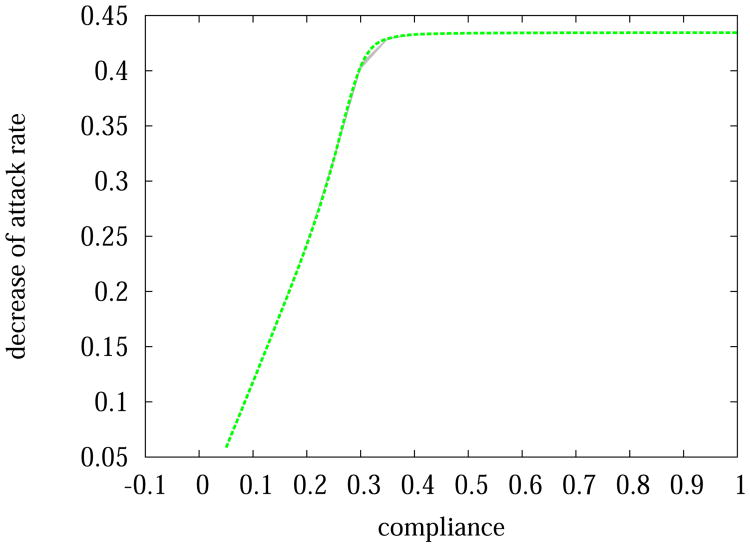
To further clarify the point, we show an example in Figure 16. When few people are vaccinated, the figure shows that it is worthwhile to vaccinate more people. But beyond 40% compliance in a 25% random subpopulation (in other words, a 10% vaccination coverage of the whole Delhi population) administrating more vaccines becomes inefficient. In fact, increasing vaccination coverage from 10% to 25% (corresponding to compliance rate increase from 40% to 100% in the randomly selected subpopulation) deceases the attack rate by less than 5%. This nontrivial observation can guide public health policy-makers to pursue other effective interventions to further reduce the attack rate.

Figure 16.

Decrease of attack rate in Delhi after applying vaccinations to 25% of population selected at random. Different compliance of people in taking the vaccination leads to very different efficacy of the vaccination. The changes of attack rate in response to the changes in compliance is nonlinear. The marginal benefit of vaccine administration is small when compliance rate is above 40%.

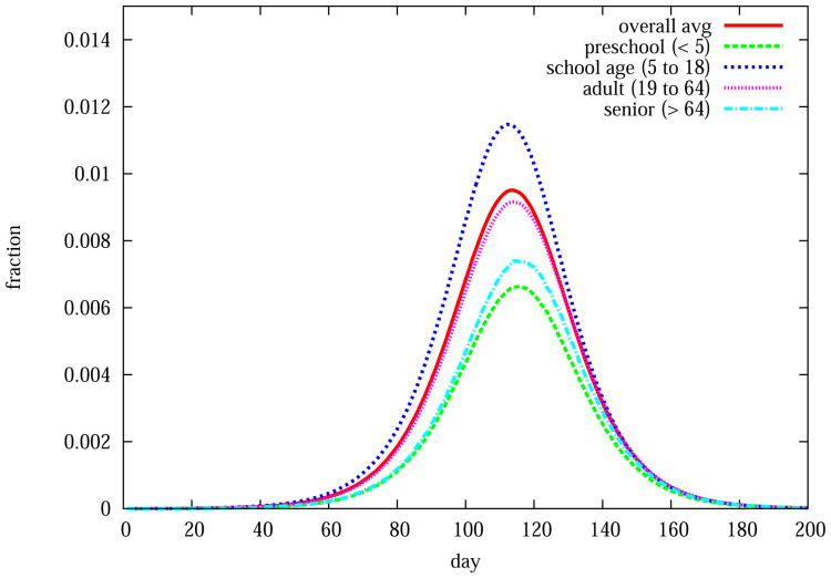
School closure and antiviral have their pros and cons. Antiviral helps reduce the attack rate more than school closure, but school closure works better in reducing the maximum number of cases on any day (peak), and in delaying the occurrence of the peak. School closure, however, is better in all three simulation outcome measures (attack rate, peak size, and peak day) than work closure. By dissecting the subpopulation structure on the basis of age and comparing the corresponding simulation outcomes, we could gain insights on controlling the spread of a disease. Figure 17 displays the epidemic curve, a plot of the fraction of people infected on each day, for each of the four subpopulations: preschool, school age, adult, and senior. Among all subpopulations, only school age individuals have an epidemic curve that is worse than the population average (solid line curve in the figure). Closing schools can avoid disease transmissions between students within schools, which explains the high effectiveness of school closure.

Figure 17.

Epidemic curves show subpopulation infection rates in the Delhi network for R₀ = 1.35. The Delhi population is partitioned into four age groups: preschool, school age, adult, and senior. Each red curve shows the fraction of people in the corresponding subpopulation infected on each day when no interventions are implemented. The solid line curve represents the infection rate for the entire population of Delhi for the duration of the epidemic.

3.3.3. Targeted-layered containment

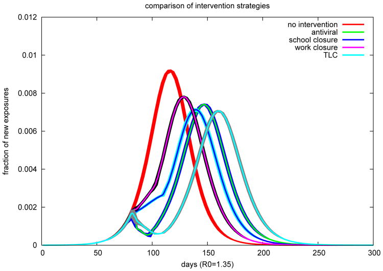
The simulated scenarios of TLCs have been described in section 2.3.3. For the disease parameters, we assume that the probability an infected individual being diagnosed is 60%. The triggering threshold for all interventions is 0.1% and the compliance is 60%. A comparison between TLC and each intervention in TLC (except targeted stay-home) is displayed in Figure 18. TLC includes all other interventions, and is naturally the most effective among all interventions.

Figure 18.

Epicurves under various intervention strategies in the Delhi network with R₀ = 1.35, including the base case where no intervention is conducted. The widths of the curves represent the standard deviation of the epicurves. The initiating threshold for all interventions is 0.1% and the compliance is 60%. TLC produces the mildest and most delayed epidemic outbreak among all interventions.

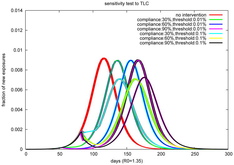
To examine the robustness of the results to our model assumptions, we test the sensitivity of the simulation results to various model parameters. For each intervention within the TLC, we experiment with compliance levels of 30%, 60% and 90%; and at the same time test for the initiating thresholds of 0.01% and 0.1%. The epidemic outcomes are listed in Table 5; and plotted in Figure 19.

Table 5.

Results of targeted-layered containment strategies in Delhi for a disease instance with R₀ = 1.35.

compliance (%)	Threshold (%)	average attack-rate (fraction)	average peak (fraction)	average peak-day
no intervention (baseline)	NA	0.434817	0.00924687	117.6
30	0.01	0.432875	0.00901022	136.967
	0.1	0.416667	0.00714037	140.633
60	0.01	0.433024	0.00902515	156.933
	0.1	0.417798	0.00713408	164.2
90	0.01	0.433257	0.00904592	168.03
	0.1	0.419244	0.00728672	176.8

Figure 19.

An experimentation of various combinations of compliance and triggering threshold for the TLC strategy yields the above epicurves. The widths of curves represent the standard deviation of the epicurves. A higher compliance leads to a more delayed outbreak. Interestingly, TLCs with an initiating threshold of 0.01% do not reduce attack rate much (see also Table 5).

The results indicate that the time when the TLC is initiated is more important than the overall compliance to the interventions. Compared to the baseline case where no intervention is conducted, a TLC initiated at an infection rate of 0.1% results in a significantly lower attack rate. On the other hand, a TLC initiated at the infection rate of 0.01% does not impact the attack rate but an increased compliance progressively delays the peak. A likely explanation is tied to the susceptible population size. When an epidemic is alleviated by an early TLC, not many people become immunized. When the disease eventually spreads out, most people are still susceptible and the population becomes severely infected.

For the same initiating threshold value, the compliance rate impacts the peak day significantly. The higher the compliance value, the more delayed the peak. At the same time, a higher compliance value does not greatly reduce the attack rate and the peak value.

4. Discussion

4.1. Sensitivity test to our synthetic network model of the Delhi network

The Delhi network was constructed using aggregated and noisy information — this aspect is inherent to the process of generating such networks. Given that the structure of the network crucially affects the disease dynamics and interventions, we perform a rigorous sensitivity analysis. Two important model parameters are the sublocation size and the location assignment algorithm. As described earlier, people within a location are divided into connected subgroups in a network view. Let sublocation size be the average subgroup size within a location; it reflects the internal structure of a location. We define for each type of locations an empirical value for their sublocation size. We note that sublocation size is a region-specific value and requires that it be adjusted based on local statistics when modeling another region. Also, we apply the gravity model to assign locations for activities. Based on observations in the real world [55], the gravity model suggests that the distance between one's home and work place or other activity locations follows an exponential distribution with density: f(x; λ) = λe^−λx where $\frac{1}{\lambda }$ is the mean distance. We choose the same experimental settings as those in Section 3. Here we assume R₀ = 1.35. We point out, however, that the observations are similar for the sensitivity experiments with the R₀ value being 1.40, 1.45, or 1.60.

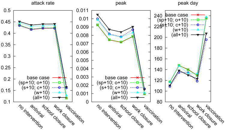
The sensitivity analysis for various sublocation sizes is shown in Figure 20. The effect of varying the sublocation size has a significant impact on the spread of the disease. Second, changing the sublocation size of some specific types of locations changes the structure of the network. For example, in the baseline network, closing schools is more effective in delaying the spread of disease as compared to closing work locations. For the network constructed after we increase the sublocation size of work places (w+10 in Figure 20), however, the effect of closing work places has the same impact as that of closing schools.

Figure 20.

Epidemics and policy efficacy in the Delhi network with various sublocation sizes (and R₀ = 1.35). Six types of locations are modeled in the Delhi network: home(h), work-place(w), school(s), college(c), shops(sh) and other(o). In the base case, we define the sublocation sizes for all locations based on empirical data. We increase the sublocation sizes for some locations in control groups. For example, (s+10, c+10) represents increasing sublocation sizes of schools and colleges by 10 and keeping sublocation sizes for the other types of locations the same as in the base case; (all+10) means increasing sublocation size for all location types (except home) by 10.

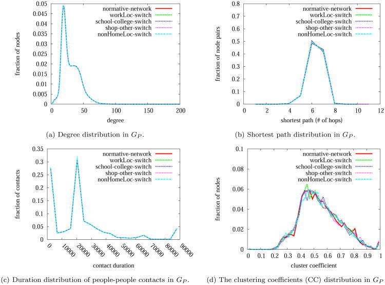
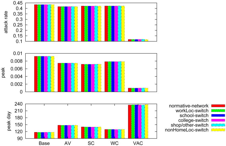
To quantify the impact of the location assignment algorithm, we switch locations for two randomly chosen people with the same type of activities. The results are summarized in Figures 21 and Figure 22. The results indicate that the network structure, the epidemic dynamics, and the intervention effectiveness are quite robust to the location assignment algorithm.

Figure 21.

Network structure perturbations for the Delhi network (G_P). Only the CC and shortest path distributions change slightly due to location switching.

Figure 22.

Impact of location switches to the Delhi network under different public health intervention policies (R₀ = 1.35). Base, AV, SC, WC, and VAC are abbreviations for “no intervention”, “antiviral”, “school closure”, “work closure” and “vaccination”. Two people are selected at random, and their daytime locations are switched (named one switch) if they are of the same type. In the control cases, “workLoc-switch” means work-places are switched randomly between workers. Other control cases are similarly named. For each case, we conduct a large number of switches to assure system convergence. However, the location switches in all cases do not change the epidemic dynamics of the underlying networks.

4.2. A comparative study of the coarse network and the detailed network

In an earlier paper [52], we developed a generic methodology aimed at data-poor areas, and generated a social contact network for Delhi based on limited data. Here we briefly compare the two networks, the term “the coarse network” refers to the one from the previous study, and “the detailed network” to the one developed in the current study. We will use these terms inter-changeably for synthetic populations and the contact network; the specific meaning will be clear from the context. The data sets used in generating the two Delhi networks are summarized in Table 6. The data and the methods used in generating these two synthetic populations and networks differ in three important ways.

1. The coarse network does not have micro-surveys for sampled households, which affects the generated synthetic population.

2. LandScan data is used to infer the location distribution in the coarse network; while exact location address data is used in the detailed network.

3. Finally, the coarse network uses an activity survey that was conducted in the United States population, which is very different than the India population. For the detailed network, activity surveys on the India population are used.

Table 6.

Data used in construction of the coarse network and the detailed network.

	the coarse network	the detailed network
demographics	India Census 2001 [36]	India Census 2001 [36] and household microdata [37]
locations	LandScan 2007 [56] school/college statistics [57, 58]	MapMyIndia: information of real locations [38]
activity	US travel survey [14]	2001 Thane household travel survey [39]; India residential area activity survey by NDSSL at Virginia Tech

As a result, the detailed network and its associated synthetic population better capture the spatial and demographic details, and the mobility patterns of the residents. The detailed network also captures the nature of time varying contact structure more accurately. We discuss this in more detail next.

Structural analysis of the coarse network and the detailed network reveals significant differences. This is summarized in Table 7. The coarse network has a much higher mean degree (76.99 v.s. 29.86) and lower edge weight (contact duration). In addition, the detailed network has a higher average clustering coefficient. These differences are significant from a disease dynamics perspective ², and the net effect is a delicate combination of these two features.

Table 7. Structural properties of several city-scale contact networks.

people-people network	No. of edges	number of nodes	Avg. degree	Avg. contact duration (minute)	Avg. CC
the coarse network of Delhi [52]	526,234,615	13,850,507	75.99	162	0.482
the detailed network of Delhi	206,787,386	13,850,507	29.86	363	0.546
the Los Angeles network [52]	459,273,880	16,228,759	56.60	141	0.389

4.3. Validation, assumptions, and limitations

Model validation is an important issue when building complex models for social systems. It is becoming increasingly well accepted that for such models, predictive validity is of limited use. In large social simulations, such predictions usually take the form of postdictions of historical information, e.g. matching the epidemic curve to historical data. Although useful in certain cases, it can also be inadequate for a number of reasons. First note that any measured real world data is incapable of capturing the range of possible outcomes; only those modes that happened in the real world appear in the measured data. Thus the process of postdiction alone is inadequate. Second, high dimensional models such as the ones discussed here have enough latitude to fit them to the relatively sparse data collected in the field. One of our goals was to develop models that have explanatory power. Another goal was to use the models for counter-factual analysis such as assessing layered containment strategies in the event of a pandemic. Substantial effort has been made to validate our complex models with these goals in mind. We discuss this briefly below.

1. Our overall process for producing synthetic populations and networks has been published in [15, 35]. The resulting synthetic population is guaranteed to be statistically identical to original data that was used to synthesize it. This includes, census and micro-survey data [36, 37, 57, 59], location data from MapMyIndia [38], activity and time use surveys [60, 61], transport networks [41] and residential surveys. Thus, for example, the total population and fraction of individuals in various age groups, the ratio of males to females, the number of school aged children, the number of workers in our synthetic population all matched the survey statistics. Similarly, the number of schools, their locations, and population density were also matched.

2. Data-driven social, behavioral, and epidemic theories were used to develop the procedural components of our model. This includes: (i) location assignment models based on generalization of gravity models [35, 39, 62–64], (ii) homophily-based assignment of activity templates to individuals [35, 64, 65], (iii) within and across host disease progression models [49, 66, 67], (iv) models of social distancing and compliance [18, 35].

3. We undertook further validation of the synthesized network. This includes structural properties of the time varying network [9, 13], visitation of individuals to locations [7], temporal variation of location occupancy [9], homophily properties in subnetworks [68], structural motifs [16, 65] etc. Note that the structural properties were not a part of the model input.

4. Finally, we performed structural validation [65, 69] through a comparison of mobility results with recently published mobility data and laws [7], epidemic dynamics, and interventions over structured networks [18].

Despite the validation, the models nevertheless have a number of limitations; future work will seek to address these constraints. Important limitations include:

1. Detailed location data in residential areas was not used. Specifically, detailed information about the precise location of each residential building was not used in the modeling process. The information will improve model resolution and allow model users to study finer grained interventions, such as quarantine of a specific building. Such data, although available, is expensive. We are investigating open source solutions to overcome this issue.

2. Massive urban slums are common in developing nations. The slums in Delhi were not well represented in our synthetic populations, due to the nature of the available data. Slum populations have several unique cultural and social attributes. Furthermore, slums are usually very dense agglomerations of households. As a result, our current simulation results may underestimate the severity of an epidemic.

3. The Thane activity survey was used as the best extant representation of the activities undertaken by individuals in Delhi. However, the small survey size as well as the discrepancy between the two cities will surely impact the precision of the simulated results. Delhi specific activity surveys should be used in future work.

4. Delhi has a large number of migrant workers, and a rapidly increasing population. We assumed the population to be fixed over the course of the epidemic. We plan to develop models for evolving synthetic populations.

5. Conclusion

Social contact networks play an important role in infectious disease epidemiology. In this paper, we described a methodology to generate high-resolution urban scale social contact networks for regions in developing countries. We focused on Delhi, the NCT in India that comprises of New Delhi and the surrounding urban areas. A key challenge in developing such a high resolution social contact network in India is the availability of data sources. We demonstrated how imputation methods developed in statistics can be used to overcome this challenge.

We then used EpiFast – a high performance computational epidemic modeling framework to study how an influenza-like illness can spread through the region. Detailed computational experiments were carried out to assess the efficacy of various interventions. Sensitivity analysis on TLC strategies reveals that the average attack rate in Delhi is more sensitive to the timing of interventions than people's compliance to the interventions, and that people's compliance to interventions greatly impacts when the epidemic peak occurs.

As a part of the paper, we have begun investigating a fundamental question in networked epidemiology — how much and what details need to be captured when constructing synthetic social contact networks. As a first step, we developed a number of structural and dynamical measures of social contact networks. These measures serve as a basis to compare two synthetic networks. For future work we will investigate the role of these structural measures on network dynamics, and more importantly on interventions.

References

- 1.WHO. Summary of probable SARS cases with onset of illness from 1 November 2002 to 31 July 2003. [Accessed: April 09, 2015]; http://www.who.int/csr/sars/country/table2004_04_21/en/index.html.
- 2.Department of Environment and Forests of India. [Accessed: March 01, 2013];State of environment report for Delhi, 2010. http://delhi.gov.in/
- 3.National Bureau of Statistics, China. [Accessed: April 09, 2015];National bureau of statistics database. http://www.stats.gov.cn/english/
- 4.Bian L. A conceptual framework for an individual-based spatially explicit epidemiological model. Environment and Planning B. 2004;31(3):381–395. [Google Scholar]
- 5.Brockmann D, Hufnagel L, Geisel T. The scaling laws of human travel. Nature. 2006;439(7075):462–465. doi: 10.1038/nature04292. [DOI] [PubMed] [Google Scholar]
- 6.Simini F, González MC, Maritan A, Barabási AL. A universal model for mobility and migration patterns. Nature. 2012;484(7392):96–100. doi: 10.1038/nature10856. [DOI] [PubMed] [Google Scholar]
- 7.González MC, Hidalgo Ca, Barabási AL. Understanding individual human mobility patterns. Nature. 2008;453(7196):779–82. doi: 10.1038/nature06958. [DOI] [PubMed] [Google Scholar]
- 8.Simini F, González MC, Maritan A, Barabási AL. A universal model for mobility and migration patterns. Nature. 2012:8–12. doi: 10.1038/nature10856. [DOI] [PubMed] [Google Scholar]
- 9.Eubank S, Kumar VA, Marathe MV, Srinivasan A, Wang N. Structure of social contact networks and their impact on epidemics. DIMACS Series in Discrete Mathematics and Theoretical Computer Science. 2006;70:181. [Google Scholar]
- 10.Mao L, Bian L. Spatial–temporal transmission of influenza and its health risks in an urbanized area, Computers. Environment and Urban Systems. 2010;34(3):204–215. doi: 10.1016/j.compenvurbsys.2010.03.004. [DOI] [PMC free article] [PubMed] [Google Scholar]
- 11.Mao L, Bian L. A dynamic network with individual mobility for designing vaccination strategies. Transactions in GIS. 2010;14(4):533–545. [Google Scholar]
- 12.Wang L, Wang Z, Zhang Y, Li X. How human location-specific contact patterns impact spatial transmission between populations. Scientific Reports. 3(1468) doi: 10.1038/srep01468. [DOI] [PMC free article] [PubMed] [Google Scholar]
- 13.Eubank SG, Guclu H, Kumar VSA, Marathe MV, Srinivasan A, Toroczkai Z, Wang N. Modelling disease outbreaks in realistic urban social networks. Nature. 2004;4:180–184. doi: 10.1038/nature02541. [DOI] [PubMed] [Google Scholar]
- 14.US Department of Transportation. [Accessed: April 09, 2015];National Household Travel Survey 2009. http://nhts.ornl.gov/
- 15.Barrett C, Beckman R, Berkbigler K, Bisset K, Bush B, Campbell K, et al. Tech Rep LA-UR-00-1725. Los Alamos National Laboratory; Los Alamos, NM: 2001. TRANSIMS: Transportation analysis simulation system. [Google Scholar]
- 16.Schneider CM, Belik V, Couronné T, Smoreda Z, González MC. Unravelling daily human mobility motifs. Journal of The Royal Society Interface. 10(84) doi: 10.1098/rsif.2013.0246. [DOI] [PMC free article] [PubMed] [Google Scholar]
- 17.Kovanen L, Kaski K, Kertész J, Saramäki J. Temporal motifs reveal homophily, gender-specific patterns, and group talk in call sequences. Proceedings of the National Academy of Sciences. 2013;110(45):18070–18075. doi: 10.1073/pnas.1307941110. [DOI] [PMC free article] [PubMed] [Google Scholar]
- 18.Halloran ME, Ferguson NM, Eubank S, Longini IM, Cummings DA, Lewis B, et al. Modeling targeted layered containment of an influenza pandemic in the united states. Proceedings of the National Academy of Sciences. 2008;105(12):4639–4644. doi: 10.1073/pnas.0706849105. [DOI] [PMC free article] [PubMed] [Google Scholar]
- 19.Bailey N. The Mathematical Theory of Infectious Diseases and Its Applications. Hafner Press; New York: 1975. [Google Scholar]
- 20.Dimitrov NB, Meyers LA. Mathematical approaches to infectious disease prediction and control. In: Hasenbein JJ, editor. INFORMS TutORials in Operations Research. Vol. 7. 2010. pp. 1–25. [Google Scholar]
- 21.Barrat A, Barthelemy M, Vespignani A. Dynamical processes in complex networks. Cambridge University Press; New York: 2008. [Google Scholar]
- 22.Germann TC, Kadau K, Longini IM, Macken CA. Mitigation strategies for pandemic influenza in the United States. Proceedings of the National Academy of Sciences. 2006;103(15):5935–5940. doi: 10.1073/pnas.0601266103. [DOI] [PMC free article] [PubMed] [Google Scholar]
- 23.Ferguson NM, Cummings DAT, Fraser C, Cajka JC, Cooley PC, Burke DS. Strategies for mitigating an influenza pandemic. Nature. 2006;442:448–452. doi: 10.1038/nature04795. [DOI] [PMC free article] [PubMed] [Google Scholar]
- 24.Ferguson NM, Keeling MJ, Edmunds WJ, Gani R, Grenfell BT, Anderson RM, Leach S. Planning for smallpox outbreaks. Nature. 2003;425:681–685. doi: 10.1038/nature02007. [DOI] [PMC free article] [PubMed] [Google Scholar]
- 25.Parker J, Epstein JM. A distributed platform for global-scale agent-based models of disease transmission. ACM Transactions on Modeling and Computer Simulation (TOMACS) 2011;22(1):2. doi: 10.1145/2043635.2043637. [DOI] [PMC free article] [PubMed] [Google Scholar]
- 26.Chao DL, Halloran ME, Obenchain V, Longini IM., Jr FluTE a publicly available stochastic influenza epidemic simulation model. PLoS Computational Biology. 6(1) doi: 10.1371/journal.pcbi.1000656. [DOI] [PMC free article] [PubMed] [Google Scholar]
- 27.Colizza V, Barrat A, Barthelemy M, Valleron A, Vespignani A. Modeling the worldwide spread of pandemic influenza: baseline case and containment interventions. PLoS Medicine. 2007;4:95. doi: 10.1371/journal.pmed.0040013. [DOI] [PMC free article] [PubMed] [Google Scholar]
- 28.Merler S, Ajelli M. The role of population heterogeneity and human mobility in the spread of pandemic influenza. Processings of Royal Society. 2010;277(1681):557–565. doi: 10.1098/rspb.2009.1605. [DOI] [PMC free article] [PubMed] [Google Scholar]
- 29.Ajelli M, Gon¸calves B, Balcan D, Colizza V, Hu H, Ramasco JJ, Merler S, Vespignani A. Comparing large-scale computational approaches to epidemic modeling: agent-based versus structured metapopulation models. BMC Infectious Diseases. 2010;10(1):190. doi: 10.1186/1471-2334-10-190. [DOI] [PMC free article] [PubMed] [Google Scholar]
- 30.Meyers LA. Contact network epidemiology: Bond percolation applied to infectious disease prediction and control. Bulletin of The American Mathematical Society. 2007;44:63–86. [Google Scholar]
- 31.Barrett CL, Bisset KR, Eubank SG, Feng X, Marathe MV. EpiSimdemics: an efficient algorithm for simulating the spread of infectious disease over large realistic social networks. SC'08. 2008:290–294. [Google Scholar]
- 32.Eubank SG. ACM Symposium on Applied Computing. Madrid, Spain: 2002. Scalable efficient epidemiological simulation; pp. 139–145. [Google Scholar]
- 33.Bisset KR, Feng X, Marathe MV, Yardi SM. Modeling interaction between individuals, social networks and public policy to support public health epidemiology. Winter Simulation Conference; 2009; pp. 2020–2031. [Google Scholar]
- 34.Bisset K, Chen J, Feng X, Kumar VA, Marathe M. EpiFast: a fast algorithm for large scale realistic epidemic simulations on distributed memory systems. Proceedings of the 23th International Conference on Supercomputing (ICS); 2009; pp. 430–439. [Google Scholar]
- 35.Barrett CL, Beckman RJ, Khan M, Anil Kumar V, Marathe MV, Stretz PE, Dutta T, Lewis B. Generation and analysis of large synthetic social contact networks. Winter Simulation Conference; 2009; pp. 1003–1014. [Google Scholar]
- 36.India-Government, India census 2001 and 2011. [Accessed: April 09, 2015]; URL http://www.censusindia.gov.in/
- 37.Desai S, Dubey A, Joshi B, Sen M, Sheriff A, Vanneman R. ICPSR22626-v8. College Park, Maryland: University of Maryland; 2008. India human development survey (IHDS), 2005; pp. 06–29. [Google Scholar]
- 38.MapMyIndia. Demographic and geo-spatial data set for Delhi. 2011 [Google Scholar]
- 39.Nehra RS. Master's thesis. University of South Florida; 2004. Modeling time space prism constraints in a developing country context. [Google Scholar]
- 40.Unicef Media. Unicef: State of the world's children 2009. [Accessed: April 09, 2015]; available online at http://www.unicef.org/sowc09/report/report.php.
- 41.Banerjee A. PhD thesis. University of South Florida; 2006. Understanding activity engagement and time use patterns in a developing country context. [Google Scholar]
- 42.Volz E. Random networks with tunable degree distribution and clustering. Physical Review E. 2004;70(5):056115. doi: 10.1103/PhysRevE.70.056115. [DOI] [PubMed] [Google Scholar]
- 43.Health.india.com. Delhi swine flu update: 37 more cases, total 457. [Accessed: April 09, 2015]; http://health.india.com/news/delhi-swine-flu-update-37-more-cases-total-457/
- 44.Bisset KR, Chen J, Deodhar S, Feng X, Ma Y, Marathe MV. Indemics: An interactive high-performance computing framework for data-intensive epidemic modeling. ACM Transactions on Modeling and Computer Simulation (TOMACS) 2014;24(1):4. doi: 10.1145/2501602. [DOI] [PMC free article] [PubMed] [Google Scholar]
- 45.Menon GI, Sinha S. Epidemiological dynamics of the 2009 influenza A(H1N1) outbreak in india. Preprint. 2010:1–5. [Google Scholar]
- 46.Jin Z, Zhang J, Song LP, Sun GQ, Kan J, Zhu H. Modelling and analysis of influenza A (H1N1) on networks. BMC public health. 2011;11(Suppl 1):S9. doi: 10.1186/1471-2458-11-S1-S9. [DOI] [PMC free article] [PubMed] [Google Scholar]
- 47.Yang Y, Sugimoto JD, Halloran ME, Basta NE, Chao DL, Matrajt L, et al. The transmissibility and control of pandemic influenza A (H1N1) virus. Science. 2009;326(5953):729–733. doi: 10.1126/science.1177373. [DOI] [PMC free article] [PubMed] [Google Scholar]
- 48.Nishiura H, Castillo-Chavez C, Safan M, Chowell G. Transmission potential of the new influenza A (H1N1) virus and its age-specificity in Japan. Euro Surveill. 2009;14(22):19227. doi: 10.2807/ese.14.22.19227-en. [DOI] [PubMed] [Google Scholar]
- 49.Tuite AR, Greer AL, Whelan M, Winter AL, Lee B, Yan P, et al. Estimated epidemiologic parameters and morbidity associated with pandemic H1N1 influenza. Canadian Medical Association Journal. 2010;182(2):131–136. doi: 10.1503/cmaj.091807. [DOI] [PMC free article] [PubMed] [Google Scholar]
- 50.Fraser C, Donnelly CA, Cauchemez S, Hanage WP, Van Kerkhove MD, Hollingsworth TD, et al. Pandemic potential of a strain of influenza A (H1N1): early findings. science. 2009;324(5934):1557–1561. doi: 10.1126/science.1176062. [DOI] [PMC free article] [PubMed] [Google Scholar]
- 51.CDC. clinical signs and symptoms of influenza. [Accessed: April 09, 2015]; http://www.cdc.gov/flu/professionals/acip/clinical.htm.
- 52.Chen J, Huang F, Khan M, Marathe M, Stretz P, Xia H. The effect of demographic and spatial variability on epidemics: A comparison between beijing, delhi, and los angeles; 2010 5th IEEE International Conference on Critical Infrastructure (CRIS), Citeseer; 2010; pp. 1–8. [Google Scholar]
- 53.Lussier J, Bank J. Tech rep. Stanford University, CA: 2011. Final report: Local structure and evolution for cascade prediction. [Google Scholar]
- 54.Leskovec J, Singh A, Kleinberg J. Advances in Knowledge Discovery and Data Mining. Springer; 2006. Patterns of influence in a recommendation network; pp. 380–389. [Google Scholar]
- 55.Barrett C, Beckman R, Khan M, Kumar V, Marathe M, Stretz P, et al. Generation and analysis of large synthetic social contact networks. Proceedings of the Winter Simulation Conference (WSC); 2009; pp. 1003–1014. [Google Scholar]
- 56.Oak Ridge National Laboratory. LandScan Data, Global Population Project at Oak Ridge National Lab. [Accessed: April 09, 2015]; http://www.ornl.gov/sci/landscan/
- 57.Delhi Department of Planning. Economic Survey of Delhi 2005-2006, Section 15. [Accessed: April 09, 2015]; http:/delhiplanning.nic.in/
- 58.University Grants Commission. India School/College Statistics. [Accessed: April 09, 2015]; http://www.ugc.ac.in/
- 59.Delhi public school, class schedule of Delhi public school. [Accessed: April 09, 2015]; http://dpsrkp.net.
- 60.Narasimhan RL, Pandey RN. some main results of the pilot time use survey in india and their policy implications. the International Seminar on Time Use Studies. 7-10 December. [Google Scholar]
- 61.Pendyala RM. Time use and travel behavior in space and time. In: Goulias KG, editor. Transportation Systems Planning: Methods and Applications. CRC Press; 2003. pp. 2–1–2–37. [Google Scholar]
- 62.Wheaton WD, Cajka JC, Chasteen BM, Wagener DK, Cooley PC, Ganapathi L, et al. Synthesized population databases: A US geospatial database for agent-based models. Methods Report (RTI Press) 10(905) doi: 10.3768/rtipress.2009.mr.0010.0905. [DOI] [PMC free article] [PubMed] [Google Scholar]
- 63.Erlander S, Stewart NF. The gravity model in transportation analysis: theory and extensions. CRC Press; Tokyo, Japan: 1990. [Google Scholar]
- 64.Bradley M, Bowman JL, Griesenbeck B. SACSIM: an applied activity-based model system with fine-level spatial and temporal resolution. Journal of Choice Modelling. 2010;3(1):5–31. [Google Scholar]
- 65.Beckman R, Channakeshava K, Huang F, Kim J, Marathe A, Marathe M, Pei G, Saha S, Vullikanti AKS. Integrated multi-network modeling environment for spectrum management. IEEE Journal on Selected Areas in Communications. 2013;31(6):1158–1168. [Google Scholar]
- 66.Nsoesie EO, Beckman RJ, Marathe MV. Sensitivity analysis of an individual-based model for simulation of influenza epidemics. PLoS ONE. 2012;7(10):e45414. doi: 10.1371/journal.pone.0045414. [DOI] [PMC free article] [PubMed] [Google Scholar]
- 67.Nishiura H, Chowell G, Castillo-Chavez C. Did modeling overestimate the transmission potential of pandemic (H1N1-2009)? Sample size estimation for post-epidemic seroepidemiological studies. PLoS ONE. 2011;6(3):e17908. doi: 10.1371/journal.pone.0017908. [DOI] [PMC free article] [PubMed] [Google Scholar]
- 68.McPherson M, Smith-Lovin L, Cook JM. Birds of a feather: Homophily in social networks. Annual Review of Sociology. 2001:415–444. [Google Scholar]
- 69.Xia H, Barrett C, Chen J, Marathe MV. Computational methods for testing adequacy and quality of massive synthetic proximity social networks; 2013 IEEE International Conference on Big Data Science and Engineering; IEEE, Sydney, Australia. 2013. pp. 1113–1120. [Google Scholar]