Population coding under normalization

Abstract

Divisive normalization of neuronal responses by a pooled signal of the activity of cells within its neighborhood is a common computation in visual cortex. From a geometrical point of view, normalization constraints the population response to high-contrast stimuli to lie on the surface of a high-dimensional sphere. Here we study the implications this constraint on the representation of a circular variable, such as the orientation of a visual stimulus. New results are derived for the infinite dimensional case of a homogeneous populations of neurons with identical tuning curves but different orientation preferences. An important finding is that the ability of the population to discriminate between any two orientations depends exclusively on the Fourier amplitude spectrum of the orientation tuning curve. We also study the problem of encoding by a finite set of neurons. A central result is that, under normalization, optimal encoding can be achieved by a finite number of neurons with heterogeneous tuning curves. In other words, increasing the number of neurons in the population does not always allow for an improved population code. These results are used to estimate the number of neurons involved in the coding of orientation at one position in the visual field. If the cortex were to code orientation optimally, we find that a small number (~5) of neurons should suffice.

Introduction

The gain control model extended the classic linear-nonlinear model of simple cells (Movshon, Thompson & Tolhurst, 1978) to account for a number of response properties, including response saturation, phase advance of temporal responses with contrast, and the results of masking experiments using plaid stimuli (Bonds, 1989, Carandini, Heeger & Movshon, 1997, Heeger, 1992, Robson, 1988). The basic idea of the model is that an initial set of responses, provided by direct input from other brain regions, gets normalized (divided) by a pooled signal of activity in the neighborhood a cell (Fig 1).

Fig 1.

Normalization of population responses. Front end linear receptive fields are followed by a half-rectifier (Movshon et al., 1978), and the resulting responses are normalized by the term $\sqrt{{\sigma }^2+{\left|\right|r\left|\right|}^2}$. (Figure modified from Carandini et al (1997)).

Progress over the last decade has shown that such normalization is a widespread computation in the brain; it can be found in the retina (Benardete, Kaplan & Knight, 1992, Shapley & Victor, 1979a, Shapley & Victor, 1979b, Shapley & Victor, 1981, Solomon, Lee & Sun, 2006), the lateral geniculate nucleus (Bonin, Mante & Carandini, 2005, Bonin, Mante & Carandini, 2006), primary visual cortex (Carandini et al., 1997, Heeger, 1992, Ringach & Malone, 2007, Rust, Schwartz, Movshon & Simoncelli, 2005), area MT (Simoncelli & Heeger, 1998), and area IT (Zoccolan, Cox & DiCarlo, 2005). Furthermore, normalization models appear to account well for the modulatory effects of attention (Reynolds, Chelazzi & Desimone, 1999, Reynolds & Heeger, 2009).

The prevalence of normalization in the nervous system must surely reflect the fact that it evolved to address a problem that arises at different stages of processing (Douglas & Martin, 2004, Douglas & Martin, 2007). From a theoretical point of view, this observation prompts a number of interesting questions. What basic principles of signal processing would lead to normalization of responses to be a critical component of neural computation? How normalization impacts the way stimuli can be encoded and processed? What are the computational capabilities of networks of normalized populations?

Some recent studies have considered how normalization modifies the statistical dependencies of neural activity, and have put forward the idea that normalization may serve to optimize the representation of natural signals (Fairhall, Lewen, Bialek & de Ruyter Van Steveninck, 2001, Olshausen & Field, 1996a, Olshausen & Field, 1996b, Olshausen & Field, 2004, Ruderman & Bialek, 1994, Schwartz & Simoncelli, 2001). Others have noted that normalization may also serve a role in decoding the activity of neuronal populations (Deneve, Latham & Pouget, 1999). Here we take complementary approach and ask not why, but how is that the representation of information constrained when carried by the signals of a normalized pool of neurons? Under what conditions are such representations optimal?

We study this problem in two scenarios that are simple enough that allow theoretical results to be obtained. First, we consider the encoding performed by a homogeneous set of neurons with identical tuning curves differing only in their preferred orientation. The main object of study is the information tuning curve (Kang, Shapley & Sompolinsky, 2004) which specifies the ability of the population to discriminate between any two orientations. When the number of neurons tends to infinity, closed form calculations can be performed that clarify the constraints imposed by normalization onto the information tuning curve. In particular, it is shown that the information tuning curve is determined by the Fourier amplitude spectrum of the tuning curve. Surprisingly, the result can be used show that the average discrimination performance of the population (measured as the average (d′)² across all possible orientation pairs) depends exclusively on the mean of the tuning curve of neurons and not at all on its shape. This has important consequences for experiments in perceptual learning that attempt to gauge how neuronal populations change during the learning process. Namely, geometric properties of local shape of the tuning curve (such as its bandwidth at half-height or maximum slope) are not the best choice when evaluating how a population’s ability to discriminate between any two orientations. Instead, its Fourier amplitude spectrum is better suited as it encodes all the information in the information tuning curve.

Second, we study the more complex situation of finite dimensional cases, where neurons are also allowed to have different tuning curves. We ask how can we best represent a circular variable in an optimal fashion in this case. The main finding is, at first, counterintuitive: normalization causes the optimal encoding to be attainable using a finite number of neurons. In other words, increasing the number of neurons in a normalized population does not always allow for an improved population code.

We then show these results can be used to estimate the number of neurons involved in the coding of orientation at any one position in the visual field from experimental data. The results show that, if the cortex were to code orientation optimally, a small number (~5) of normalized neurons would suffice.

These findings demonstrate that normalization imposes important constraints on the coding of information and, giving its incidence in cortical circuits, it should be incorporated as an integral component in formal models of population coding.

Results

A geometric view of normalization

The normalization model we adopt is one that has been used widely to model the responses of simple cells in primary visual cortex (Carandini et al., 1997, Heeger, 1992):

$${\widehat{r}}_i=r_i/\sqrt{{\sigma }^2+{\left|\right|r\left|\right|}^2}i=0,1,\cdots ,N-1$$ (1)

Here, r_i represents the initial response of neuron i to a stimulus, r = (r₀, r₁, · · ·, r_N−1) is a vector describing the response of the N cells in the population, ||r|| is the Euclidian norm of the vector, σ is the semi-saturation constant, and r̂ = (r̂₀, r̂₁, · · ·, r̂_N−1) is the vector of normalized responses. Our first observation is simple: for strong stimuli, for which ||r|| ≫ σ, the normalized population response lies on a hyper-sphere, S^N−1. This means that in general the problem of encoding under normalization becomes one of defining a map from a given stimulus space to a high-dimensional sphere, the dimension of which is determined by the number of neurons at hand. A few examples demonstrate how this fact leads to some interesting theoretical problems.

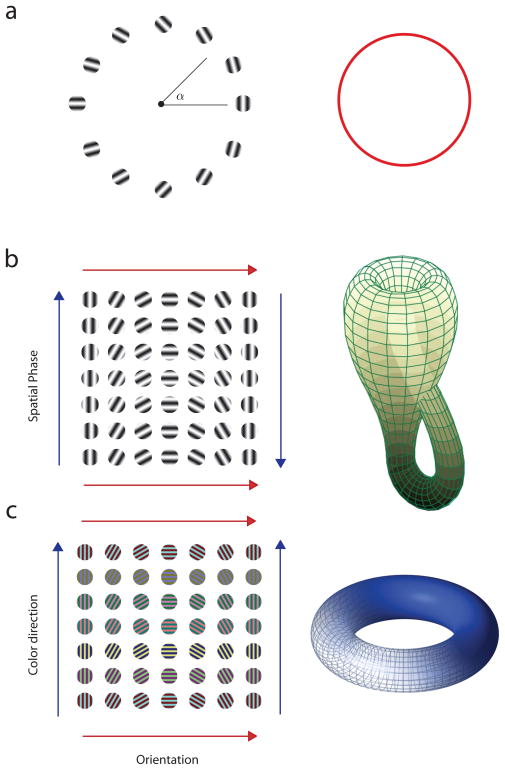
Consider first the coding of a circular variable, which we will discuss in detail below. This a problem confronted by the nervous system in several contexts, including the coding of the orientation or direction of motion of a visual stimulus, the color hue of a surface patch, wind direction, reaching direction, and heading direction with respect to magnetic north. In all these cases, the domain of the stimulus can be associated to unit circle. Any point on the circle defines can be associated with the value of the variable under consideration (Fig 2a). Thus, the problem of encoding a circular variable by a normalized population of N neurons amounts to defining a map that takes the unit circle into the a (N − 1) -sphere,

Fig 2.

Topology of stimulus spaces. Different stimulus spaces have different topologies. Under normalization all these different objects must be immersed in high dimensional spheres, (a) A circular variable is topologically equivalent to a circle. (b) Orientation and spatial phase of sinusoidal gratings is topologically equivalent to a Klein bottle. (c) Orientation and color direction is topologically equivalent to a torus.

$$f:S^1\to S^{N-1}.$$ (2)

Studying the property of these maps, and how one could obtain some that are optimal in some sense, is the central topic of our study.

Another interesting situation arises when we consider the joint coding of the orientation and the spatial phase of a sinusoidal grating (Fig 2b). This stimulus space represents a Klein bottle, a fact that may not be entirely evident at first (Carlsson, Ishkhanov, DaSilva & Zomordian, 2007, Singh, Memoli, Ishkhanov, Sapiro, Carlsson & Ringach, 2008, Swindale, 1996, Tanaka, 1995). One way to show this is by plotting the individual gratings corresponding to the various combinations of the parameters (Fig 2b). One can then see that gratings on the top and bottom rows are identical to each other, as indicated by the matching directions of the two red arrows. If we wanted to match these two arrows one on top of the other all we need to do is roll the rectangle of gratings into a cylinder. On the other hand, the stimuli on the left and right columns are the same but reversed in order, as indicated by the directions of the blue arrows. To match the directions of the blue arrows once we have rolled the space into a cylinder we would need to puncture the cylinder in 3D space, but it turns out that it can be done in 4D without trouble (Fig 2b). The resulting object is a Klein bottle. Thus, the problem of mapping the orientation and spatial phase of a grating onto the normalized population of cells amounts to defining an embedding of the Klein bottle into the (N−l) -sphere.

A final example is the joint coding of orientation and color hue (Johnson, Hawken & Shapley, 2008) (Fig 2c). Here, as one can infer by the direction of the arrows, the resulting object is a torus, which is obtained by rolling the space into a cylinder and then gluing the ends together. Implementing a population code that maps orientation and color hue to a normalized population of neurons is thus equivalent to the embedding of a torus in a high-dimensional sphere.

These examples illustrate that interesting geometrical and topological problems arise when we consider the representation of visual information via normalized population of neurons. In what follows, we take a first step to gain some insight into the constraints imposed by normalization we being by considering a very simple case of orientation tuning (Benyishai, Baror & Sompolinsky, 1995, Salinas & Abbott, 1994, Seung & Sompolinsky, 1993).

Representation of a circular variable by an infinite population of homogeneous neurons

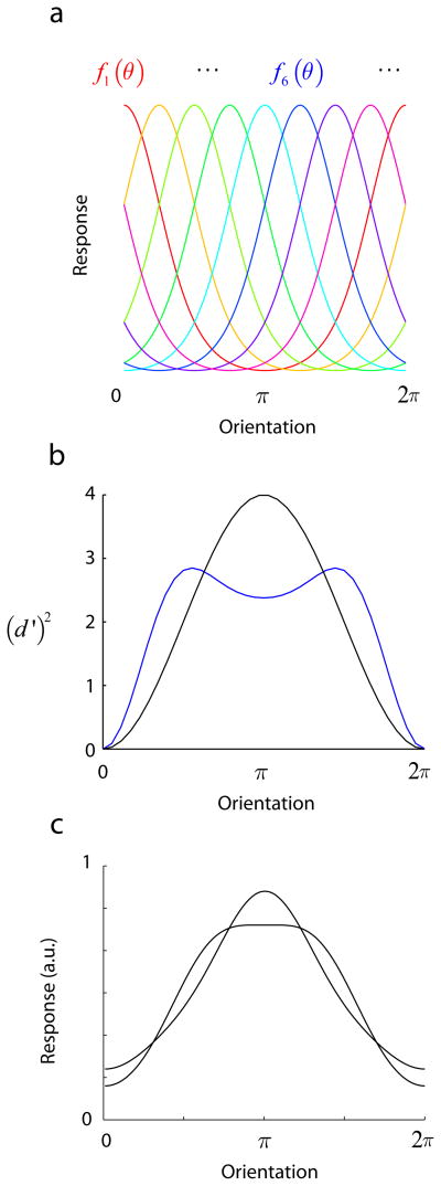
Consider a set of N neurons whose orientation tuning curves are identical but differ only in their preferred orientations, which we assume to be evenly spaced around the circle (Fig 3a). The tuning curve of the i–th neuron is given by f_i(θ) = C_N f(θ − 2πi/N) with i = 0,1, · · ·, N − 1. The population response to a given orientation will be denoted by f(θ) = (f₀(θ), f₁(θ), · · ·, f_N−1(θ)). Without loss of generalization, we assume that normalization implies the length of this vector equals one, ||f (θ)|| = 1. For a given tuning curve shape, the value of C_N can be picked to ensure this normalization constraint as the number of neurons in the population changes. We further assume that the output of each neuron is corrupted by i.i.d. Gaussian noise.

Fig 3.

A simple model for the population coding of a circular variable. (a) A number of neurons with identical tuning curves but different orientation preferences are distributed around the circle. We study the limit when the number of neurons goes to infinity and the population curve has a norm of one. (b) The information tuning curve measures the ability of the population to discriminate between any two orientations. Due to symmetry, the value of d′ is only dependent on the difference between the two orientations, Δθ. The figure shows two sample curves obtained with a cosine tuning function (black line) and with a sharper bell-shape tuning curve (blue line). (c) Two orientation tuning curves that have the same amplitude spectrum but different relative phases. Despite the fact that their shapes are different (for example the bandwidth at half-height differs substantially), these two tuning curves generate exactly the same population code (that is, the same information curve).

Under these simple conditions the ability of an ideal observer to discriminate two orientations α and β based on the population response is proportional to d′(α, β) = ||f(α) − f (β)||. However, we will be working with a quantity that is more amenable to computation, the squared value of d′, which is proportional to other measures of information used in the past such as Fisher information (for small angles) and the Chernoff distance (Kang et al 2004, Seung & Sompolinsky, 1993).

In the limit, when the number of neurons N → ∞ its value becomes (Kang et al., 2004, Seung & Sompolinsky, 1993),

$$\begin{array}{l}{lim}_{N\to \infty }{d}^{\prime }{(\alpha ,\beta )}^2={lim}_{N\to \infty }{\left|\right|\mathbf{f}(\alpha )-\mathbf{f}(\beta )\left|\right|}^2\\ ={lim}_{N\to \infty }{C}_N{\sum }_{i=1}^N{\left(f_i(\alpha )-f_i(\beta )\right)}^2\\ =\underset{0}{\overset{2\pi }{\int }}{\left[f(\theta -\alpha )-f(\theta -\beta )\right]}^{2}d\theta \\ ={\left|\right|f(\theta -\alpha )-f(\theta -\beta )\left|\right|}^2\end{array}$$ (3)

where we used the fact that for large N the value of C_N ~1/N for the normalization constrained, ||f(θ)|| = 1, to be maintained for all N. Thus, in the limit, the population response to a given orientation has a shape identical to the orientation tuning curve centered at the neuron with that preferred orientation. Thus, f(θ − α), which is the tuning curve for a neuron with preferred orientation α, also becomes the response of the population with preferred orientations θ to a stimulus of orientation α. The equation above expresses the squared Euclidean distance between two population responses evoked by angles α and β. For large number of neurons the normalization of the population response is equivalent to normalization of the tuning curve, ||f (θ)|| = 1.

We can now calculate (d′)² by representing the orientation tuning function with its Fourier series, f(θ) = Σ_kc_kexp(ikθ). We obtain,

$$\begin{array}{l}{d}^{\prime }{(\alpha ,\beta )}^2={\left|\right|f(\theta -\alpha )-f(\theta -\beta )\left|\right|}^2\\ =2\pi {\sum }_k{\mid c_k\mid }^2{\mid 1-exp(ik\mathrm{\Delta }\theta )\mid }^2\\ =4\pi {\sum }_k{\mid c_k\mid }^2(1-cos(k\mathrm{\Delta }\theta ))\\ =2{\left|\right|f\left|\right|}^2-4\pi {\sum }_k{\mid c_k\mid }^{2}cos(k\mathrm{\Delta }\theta )\end{array}$$

$$d^{\prime }{(\mathrm{\Delta }\theta )}^2=2-4\pi {\sum }_k{\mid c_k\mid }^{2}cos(k\mathrm{\Delta }\theta )$$ (4)

The calculation shows that (d′)² depends only on the difference between the orientations, Δθ = α − β (Fig 3b). This result is a direct consequence of the symmetric arrangement of the tuning curves (Fig 3a) and their homogeneity. We refer to this property as translation invariance. The function d′ (Δθ)² is called the information curve and provides the full information about the ability of the population code to discriminate between two orientations that differ by Δθ (Kang et al., 2004, Sompolinsky, Yoon, Kang & Shamir, 2001) (Fig 4a). The above expression for d′ (Δ θ)² immediately leads to a few interesting results.

Fig 4.

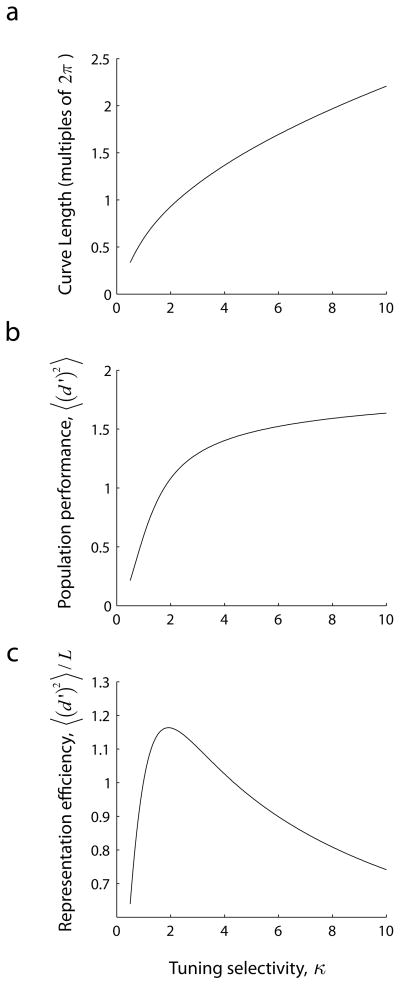
Optimal coding for von-Mises orientation tuning curves. In the case of von-Mises tuning curves the (a) length of the curve (or receptive field complexity), (b) population code performance, and (c) their representation efficiency (the ratio between performance and complexity) can be calculated in closed form. The optimal representation is achieved at a value of κ ~ 1.92. Thus, efficiency peaks at some moderate bandwidth.

The information curve is determined by the amplitude spectrum of the orientation tuning curve

Note that d′ (Δθ) depends only on the amplitudes of the Fourier coefficients of the orientation tuning curve, |c_k|. In other words, the relative phases of the Fourier components, which have a strong impact on the shape of the tuning curve, do not affect the information curve at all. This means that tuning curves that that have the same amplitude spectrum, but different phases and shapes, will produce exactly the same information curve (see Fig 3c for an example).

This result is important because it implies that in order to evaluate changes in the ability of neuronal populations to discriminate between any two orientations measures of geometric properties of local shape of the tuning curve (such as its bandwidth at half-height or maximum slope), are not necessarily the best choice. Instead, the amplitude spectrum of the tuning curves is a more relevant quantity. This is relevant to many studies where we might need to evaluate the ability of neuronal populations to code orientation before and after perceptual learning.

Fourier series of the information curve

In addition, Eqn (4) can be seen to represent the Fourier series of d′ (Δθ)². This provides a helpful tool to synthesize/design tuning curves to implement any desired information curve. This could be done as follows: (a) compute the amplitude spectrum of the desired information curve, (b) take the square root of the coefficients, (c) synthesize a tuning curve with the resulting coefficients as their Fourier amplitudes with arbitrary relative phases. An large population of such neurons will then have the desired information curve.

Constraint on average discrimination performance

By integrating Eqn (4) w.r.t. Δθ one obtains that the mean value of d′(Δθ)² is determined exclusively by the mean of the orientation tuning curve, c₀:

$$\langle d^{\prime }{(\mathrm{\Delta }\theta )}^2\rangle =2-4\pi c_0^2$$ (5)

Surprisingly, this means that the actual shape of the tuning curve does not influence the mean discrimination of the population. Two populations based on tuning curves of different shape, but with the same mean, will have the same average discrimination performance. If we consider a class of tuning functions all with the same mean, the above constraint implies that we cannot improve sensitivity for some range of Δθ without sacrificing performance in another. For example, we cannot improve the discrimination of nearby angles without deteriorating the population’s ability to discriminate between large angles (see also Kang (2004)). To illustrate this point, the information curves in Fig 3b were generated by with two tuning curves with the same mean. While the blue tuning curve leads to better performance at small angles, it leads to worse performance at larger angles.

Quadratic behavior for small angles

For small angular differences Eqn (4) simplifies to:

$$d^{\prime }{(\mathrm{\Delta }\theta )}^2\simeq {\left|\right|f^{\prime }\left|\right|}^2\mathrm{\Delta }{\theta }^2.$$ (6)

This can be obtained by substituting the small angle approximation cos(kΔθ) ≈ 1 − (kΔθ)²/2 in Eqn (4) (see also (Seung & Sompolinsky, 1993)). This means that the information curve near the origin is quadratic and determined by the value of ||f′||.

The length of the population curve

The value of ||f′|| also determines the length of the curve onto which the unit circle is mapped, which equals:

$$L={\int }_0^{2\pi }\left|\right|f^{\prime }\left|\right|d\theta =2\pi \left|\right|f^{\prime }\left|\right|$$ (7)

Note that in the present model the value of ||f′|| is constant, meaning that the ability of the population to discriminate between two nearby angles θ and θ + Δθ is independent of θ. The length of the curve directly reflects how fast the population vector varies with small changes in the input. The more sharply tuned the tuning curve is the larger ||f′||. Therefore, the length of the curve represents a measure of tuning selectivity.

Intuitively, the wiring of receptive fields with high selectivity for orientation is more demanding than the wiring of broadly tuned receptive fields. Thus, in some sense the value of L also expresses the ‘complexity’ of the receptive fields in the population. As an example, consider the class of two-dimensional Gabor filters. Sharp tuning is achieved as the number of effective subregions increases or if their individual aspect ratio is increased (Jones & Palmer, 1987, Ringach, 2002). The wiring of receptive fields with increasingly elongated subregions or higher number of subregions becomes more complex as these numbers go up.

At the same time, recall that 〈 (d′)² 〉 provides a measure of the ability of the population to encode a circular variable. An optimal representation would be one that attains the maximum possible values of 〈 (d′)² 〉 while keeping the complexity of the receptive fields as low as possible. One way to do this is by posing the problem of maximizing the ratio 〈 (d′)²〉/L.

Optimal representation for von-Mises tuning curves

This optimization problem can be solved analytically when we restrict the class of tuning functions to those having the same shape as that of a von-Mises distribution, so that f(θ) = Aexp(κ cos (θ)). The value of A is such that normalizes the population, ||f(θ)|| = 1. Then, the values of 〈 (d′)² 〉 and L can be calculated by making use of the identity, $exp(\kappa cos\theta )=I_0(\kappa )+2{\sum }_{n=1}^{\infty }{I}_n(\kappa )cos(k\theta )$, where I_n (z) is the modified Bessel function of the first kind. The result is then,

$$L=2\pi \sqrt{\frac{\kappa I_0{(\kappa )}^2}{2I_0(2\kappa )}}\text{and}\langle {(d^{\prime })}^2\rangle =2-\frac{2I_0{(\kappa )}^2}{I_0(2\kappa )}$$ (8)

Both variables are monotonically increasing with κ, but their ratio has an maximum at intermediate value of κ ≈ 1.92 (Fig 4). This corresponds to a half-bandwidth at half-height of ~25 deg, which is similar to the empirical average (Ringach, Shapley & Hawken, 2002).

The reason behind this result is that the length of the curve can be made arbitrary large (Fig 4a), while the ability of the population to code for orientation under normalization is limited due to the fact that the space is bounded and 〈 (d′)² 〉 ≤ 2 (Fig 4b). This is explained by noticing that as κ increases the tuning curves become narrower and narrower, approximating delta functions. This means that the dot product of any two population responses corresponding to two different orientation angles will approach zero and, in the limit, they will be orthogonal to each other. The squared Euclidean distance between any two such populations responses, each with a norm of one, is 2 (Pythagoras), which is an upper bound for 〈 (d′)² 〉. Under normalization, therefore, an optimal trade-off between population performance and the complexity of receptive fields is achieved for some intermediate bandwidths.

Replication of a circular variable by a finite population of neurons

Having gained some insight into the effects on normalization in the case of large number of neurons with identical tuning curves we now turn our attention to how coding might be affected when the number of neurons in the population is finite and their tuning curves heterogeneous. If the population has N neurons, we are looking for maps of the unit circle onto the sphere S^N−1. The only parameter in the problem is the length of the curve on the sphere, L.

We study this problem numerically by parametrizing the maps with a finite set of points. Consider a set of M points, {x_i} equally spaced around the unit circle (Fig 5a), representing a set of equally spaced orientations. Assume these points are mapped onto the set of points, y_i ∈S^N−1 (Fig 5b).

Fig 5.

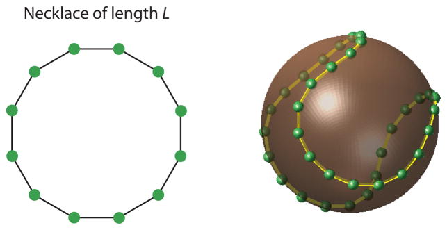
The problem of mapping the unit circle onto a sphere in an optimal fashion, (b) Our formulation considers the intuitive problem of finding the minimum energy configuration of a “necklace” with beads of equal charge, (b) Example of an optimal solution for S² and a length L = 1.6 × 2π.

We will also assume that the ability of the population to discriminate between nearby orientations is the equal around the circle by imposing the additional constraint

$$\Vert y_i-y_{(i+1)modM}\Vert =L/Mi=0,1,\cdots ,M-1$$ (9)

With this constraint in place, one can visualize the problem as that of wrapping a necklace with N beads, where adjacent beads are linked by rigid rods of length L/M, onto the sphere S^N−1.

Next, we need a measure that will capture the ability of the population to discriminate between orientations. Intuitively, we want the points y_i to be as far apart from each other as possible. One possible measure of their separation is the energy function,

$$W=\frac{1}{2}\sum _{i\ne j}\frac{1}{\Vert y_i-y_j\Vert }$$ (10)

which has a simple physical interpretation. Namely, if we consider y_i to be the coordinates of particles with the a positive unit charge, the above function measures the potential energy of the configuration. If we were to place such a necklace with charged particles on a sphere, its configuration would evolve to the one that achieves the minimum potential energy. We can then define the optimal representation as one that achieves the minimum energy configuration, arg min_{yi} W. Other criteria are possible, such as maximizing the volume of the convex hull of the beads, but they do not admit simple physical interpretations and are not studied here.

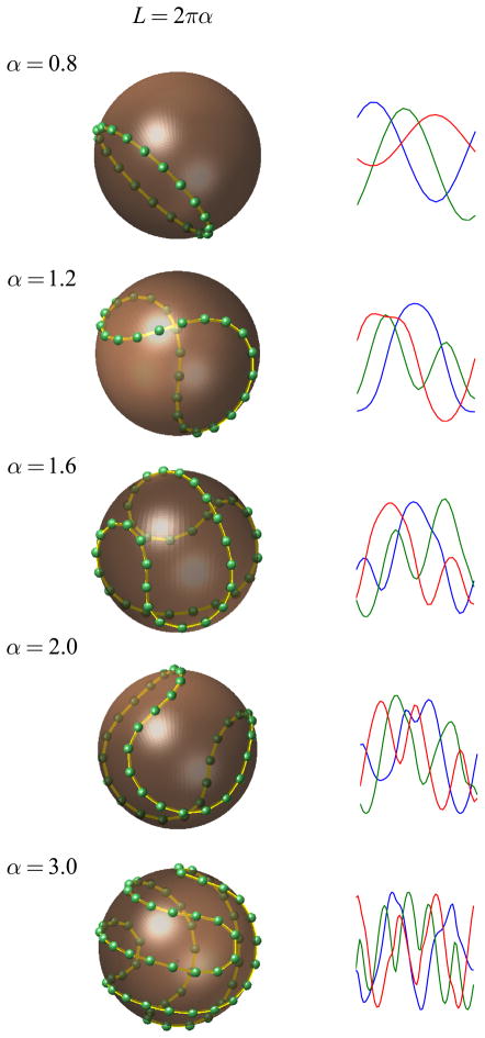
To explore the properties of minimum energy solutions we begin by visualizing the results for S². When the length of the necklace is less than 2pi;, the circumference of sphere, then the solutions are simply circles on the surface of the sphere (Fig 6, top panel). The interesting solutions arise when the length of the curve is larger than 2pi; (when α > 1). In that case, we see the curve starting to deform first into a saddle shape, then into a baseball seam, and finally develops a twist (Fig 6, bottom panels).

Fig 6.

Optimal solutions in S² and sample tuning curves implementing them. Left column. Minimum energy configurations for S² and a range of curve lengths. The optimal curves evolve from simple circles to saddle shapes and finally develop a twist bifurcation. Right column. Example of tuning curves that implement the population code (curve) on the left. As the length of the curve increases the tuning curves develop additional peaks in addition to the one at its preferred orientation.

The solutions can be determined up to a rotation or reflection, as these transformations do not change the mutual distances between the charges and, therefore, neither the energy of the configuration. For any given solution, a set of tuning curves can be ‘read’ as the Cartesian coordinates of the curve described by the necklace. Sample tuning curves for the three-dimensional case are shown in the right column of Fig 6. When the length is less than 2pi; all tuning curves are cosine shaped. As soon as the necklace length crosses the 2pi; threshold some of the curves can develop Mexican-hat shapes, which have a secondary peak orthogonal at an angle to its preferred orientation. Note that in the finite dimensional case the optimal solutions generally lead to a set of tuning curves with different shapes. As the length of the necklace increases further the curves become multi-peaked.

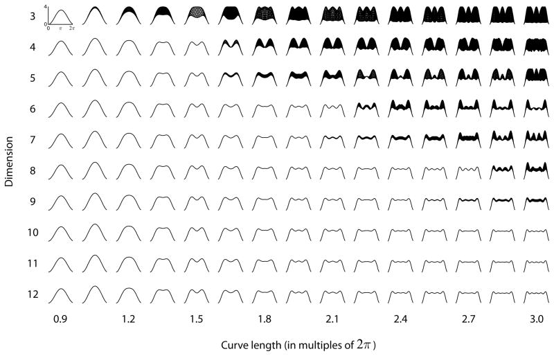
The distance between two charges d_ij = ||y_i − y_j|| is proportional to the discriminability of the orientations represented by these points and, for each reference orientation j we can compute an information tuning curve d_ij = ||y_i − y_j||. The information curves corresponding to the optimal configurations for a range of dimensions and curve lengths are shown in the panels of Fig 7. If only one curve is visible in a panel, it is because they are all identical and superimpose one on top of another. This means that, as in the case of a homogeneous population of neurons, the information tuning curve is only a function of the difference between the orientation angles -- that is, translation invariance holds.

Fig 7.

Information tuning curves corresponding to the optimal (minimum energy) configuration for various combination of dimension (y-axis) and curve length (x-axis). Note that curve length is expressed as multiples of 2π.

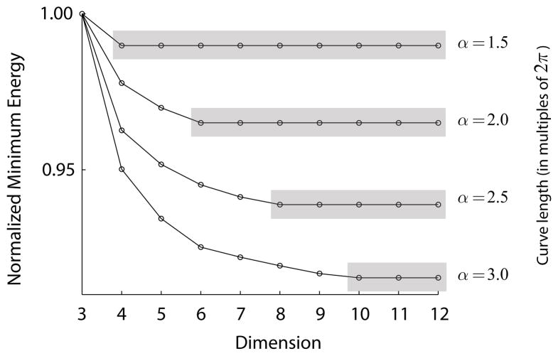
Note that translation invariance of optimal solutions holds only for certain combinations of dimensions and curve lengths. In particular, for any given dimension (the number of neuros minus one), there is a upper bound beyond which optimal solutions are no longer translation invariant. The simulations also indicate that for any given curve length, there is a dimension after which the information tuning curves corresponding to the optimal configuration do not change any more. This means that adding more dimensions (i.e. neurons) to the population does not allow for a better (smaller energy) population performance.

This can be best seen by plotting the (normalized) minimum energy as a function of dimension with the length of the curve as a parameter (Fig 8). Each curve corresponds to a different curve length. For each curve, there is a finite dimension after which the energy remains constant. After this point, adding more dimensions leads to the same solution. As elaborated below, we conjecture that for even dimensions, d = 2k, the maximum curve length for which the minimum energy solutions in S^d are translation invariant is given by $L_{max}(k)=2\pi \sqrt{(k+1)(2k+1)/6}$.

Fig 8.

Normalized minimum energy for curves of various lengths as a function of dimension. The reason for the normalization is that the number of “beads” used in the simulations increase with the length of the curve, so as to maintain a good spatial resolution. We thus normalized the data to the energy for a dimension of 3. The longer the curve the more we gain (in terms of reducing the relative energy) by adding extra dimensions (neurons) in the encoding. Yet, for any given curve length there is a dimension after which no further gains are attainable (shaded regions).

There is a simple intuitive explanation for this finding. Without normalization the addition of additional neurons with uncorrected noise would be expected to improve the discriminability. However, with normalization present, the addition of a neuron comes at the expense of increasing the denominator in Eqn (1), thereby reducing the responses of all neurons. This increased suppression of the responses prevents the population from increasing the performance of its population code.

A simpler representation of translation invariant solutions

We have parameterized the mapping from the unit circle to the sphere by the position of a finite set of charges, which has M × (d−2) parameters (due to normalization and nearest neighbor constraints). One may ask if there are simpler representations of these curves, in particular in the range of lengths and dimensions for which the solutions are translation invariant. It can be shown that for even dimensions, d = 2k, these solutions have the form:

$$\mathbf{y}(\theta )=(a_{1}cos\theta ,a_{1}sin\theta ,\cdots ,a_{k}cosk\theta ,a_{k}sink\theta )$$ (11)

a simpler representation with only d/2 = k parameters (a derivation can be found in (Fuster, Costa & Ballesteros, 1989, Vaishampayan & Costa, 2003)). Note also the norm of the population vector is then

$${\left|\right|\mathbf{y}\left|\right|}^2={\sum }_{m=1}^k{a}_m^2=1$$ (12)

with the last equality being the requirement for normalization. The length of the curve is L = 2π||y′||, and using the above representation we get ${\left|\right|{\mathbf{y}}^{\prime }\left|\right|}^2={\sum }_{m=1}^k{m}^2{a}_m^2$, so that $L=2\pi \sqrt{{\sum }_{m=1}^k{m}^2{a}_m^2}$.

The information curves for these cases can be readily computed, from Eqn (11), to be

$${\Vert \mathbf{y}(\theta )-\mathbf{y}(\theta +\mathrm{\Delta }\theta )\Vert }^2=2-2{\sum }_k{a}_k^{2}cos(k\mathrm{\Delta }\theta )$$ (13)

which we immediately recognize as equivalent to Eqn (4), describing the translation invariant curves for the infinite dimensional case with a_k = 2pi;|c_k|.

To verify the equivalence of the solutions we searched for the minimum energy configurations for a parameterized set of charges (M × (d − 2) parameters), or when the same number of charges are sampled from the curves in Eqn (11), so that

$${\mathbf{y}}_i=\left(a_{1}cos(2\pi i/M),a_{1}sin(2\pi i/M),\cdots ,a_{k}cos(2\pi ik/M),a_{k}sin(2\pi ik/M)\right)i=0,\cdots ,M-1$$ (14)

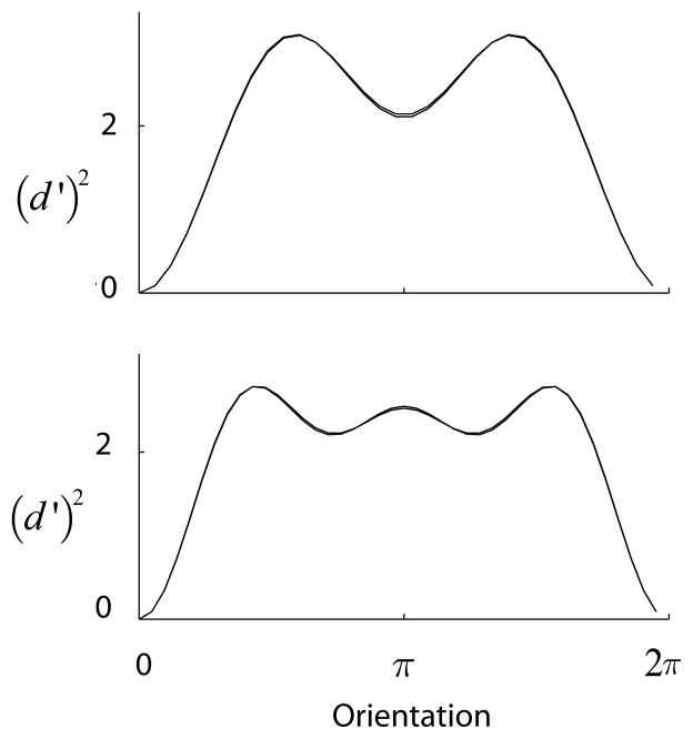
(which has d/2 = k parameters). The results, as expected, were identical (Fig 9).

Fig 9.

Verification of translation invariant solutions. Two examples showing the optimal information tuning curves obtained for two different combinations of lengths and dimensions for the optimization of the location of the charges or the Fourier coefficients of the curve. The similarity between the curves in the two cases makes it look as if there is only one curve in each case, verifying that both formulations lead to the same result.

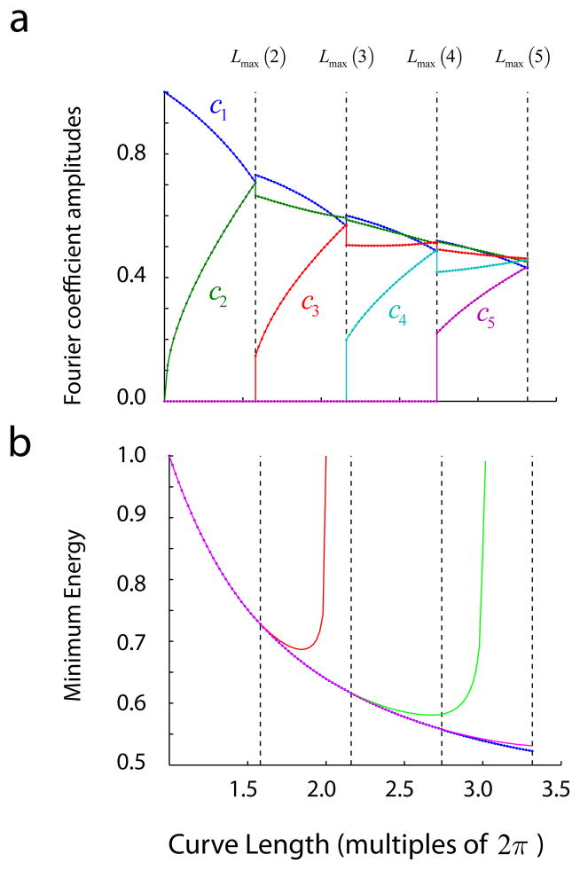
Given this representation of translation invariant solutions we can now ask how is that the Fourier coefficients of the optimal solutions vary as a function of the length of the curve and the dimension of the sphere. Fig 10a shows the optimal Fourier coefficients as a function of curve length. The vertical lines denote the boundaries given by L_max (k) for k = 2,3,4,5. One can see that up to L_max(2) ≈ 1.58 only the optimal solutions can be attained by varying the first two harmonics, a₁ and a₂, while all the other ones are zero. That means that the optimal solution lives in S⁴ requiring a population of 5 neurons. Adding more neurons to the population to encode a curve with a length smaller that L _max (2) would be a misuse of resources, as the energy cannot be reduced any further. A transition occurs as the length of the curve crosses the boundary imposed by L_max (2), after which the optimal solution calls for a non-zero third harmonic coefficient, a₃. Then, up until the curve length meets its next boundary at L_max (3) ≈ 2.16, the optimal solutions live in S⁶ requiring a total of 7 neurons, and so on. Despite the discontinuities in the Fourier coefficients as we cross these boundaries, the minimum energy is smooth (Fig 10b). If one attempts to find the optimal solutions for lengths higher L_max (2) constrained to having only the first two coefficients being non-zero, the minimum energy achieved diverges from the optimal right after L_max (2) (Fig 10b, red curve). Similar curves are obtained if we restrict the solutions to the first three harmonics when the length crosses L_max (3) (Fig 10b, green curve), or when we restrict the solutions to the first four harmonics when the curve length crosses L_max (4) (Fig 10b, blue curve).

Fig 10.

Dependence of optimal Fourier coefficients and minimum energy as a function of curve length. (a) Values of the optimal Fourier coefficients as the length of the curve increases, with clear transitions for the values corresponding to L_max(k). (b) Dependence of minimum energy as a function of curve length.

The expression for $L_{max}(k)=2\pi \sqrt{(k+1)(2k+1)/6}$ (the maximum length for which solutions are invariant for a given dimension) is presently a conjecture. By sharing the intuition that led to its formulation it may help the reader develop a formal proof. One key question is what is the smallest energy configuration one could possible obtain for an embedding onto a given dimension S^2k. The symmetry of the problem on the mutual distances, d_ij would suggest a minimum is attained when these distances are equal to each other. We can now rely on the fact that we know how to design orientation tuning curves to implement a desired information curve. Consider the family of information curves given by (d′)²(Δθ) = 0 if |θ| ≤ ε and 2 otherwise. For a given ε the best (in the mean squared sense) approximation of this tuning curve is by a truncated Fourier series of this function with the desired number of coefficients (dimension) and, as ε → 0, it is easy to verify that the Fourier coefficients will tend to have the same amplitude. Recalling that the length of the curve is given by $L=2\pi \sqrt{{\sum }_{m=1}^k{m}^2{a}_m^2}$ and that normalization implies $\sqrt{{\sum }_{m=1}^k{a}_m^2}=1$, then if the minimum is achieved when all the Fourier coefficients are equal to each other, this means that they are all $a_m^2=1/k$. Substituting this value in the length we obtain $L_{max}(k)=2\pi \sqrt{(k+1)(2k+1)/6}$. The reason this argument cannot be considered a proof is that it is not obvious that the best approximation to the ideal information curve in the mean square sense is also the one that leads to the minimum energy configuration. Thus, for now, we need to refer to the formula for L_max (k) as a conjecture, although its validity seems to be supported by the numerical simulations.

Experimental results

The most direct application of these results is an attempt to estimate the length of the curves in experiment data. We used a set of data previously published, where multi-electrode array recordings were used to measure the responses of neuronal populations to oriented sinusoidal gratings in macaque primary visual cortex (Nauhaus & Ringach, 2007). In each array implant, a subset of electrodes yielded single unit activity (ranging from 25–60 across the different arrays). The response of the population to a set of equally spaced orientation angles can be represented by a population vector r = (r₁, r₂, · · ·, r_N), where r_i is the fluctuation of the firing rate of the i-th cell around its mean. The first result is that the population was indeed approximately normalized, as the norm of the population vector fluctuates about its mean by about 10% as the orientation changes round the clock. After normalizing each population response by the mean norm we can estimate the length of the curve as the sum of the Euclidean distances among neighboring orientations, yielding a value of L = 1.34 ± 0.07 (n = 5 array implants, mean ± s.d.) This is a relatively low number and it means that if the cortex were to represent a curve of such length optimally using a normalized population of cells, then no more than 5 neurons are required, as 1.34 is less than L_max (2) ≈ 1.58.

Discussion

We have studied some of the implications of normalization for population coding from a geometric point of view. We noted that normalization constraints the population vector to lie on a sphere and that some stimulus spaces are represented by other topological classes, such as a Klein bottle or a torus. Population coding under normalization can then be though as finding embeddings of these objects into higher dimensional spheres, posing some interesting theoretical questions. We concentrated on the question of how to wrap a string of a given length on a hyper-sphere, which is the problem corresponding to the encoding of a circular variable with a normalized pool of neurons. A number of new results for the simple case of an infinite population of homogeneous neurons were described. Among them was a basic relationship between the information tuning curve and the Fourier coefficients of the orientation tuning curve. From here, a relationship between mean performance (the integral of the information tuning curve) and the mean of the orientation tuning curve was derived. One consequence of normalization is that it places a limit on performance of the code, due to the resulting limits on the diameter of the encoding space (Fig 4). Thus, it does not pay off to design increasingly complex receptive fields with sharper tuning curves, as an investment in receptive field complexity will not be returned as a worthwhile payoff in discrimination performance. The optimum encoding is attained for a moderate choice of orientation tuning bandwidth (Fig 4).

We also considered a scenario where a the encoding of a circular variable is done by a finite number of neurons with (possibly) heterogeneous orientation tuning curves. Here, we defined optimality as the minimum energy configuration of a necklace of beads, linked by rigid segments, each having equal charge. This problem is a generalization of the classic Thompson problem of the distribution of charges on a sphere (Thomson, 1904) and other manifolds (Borodachov, Hardin & Saff, 2007, Borodachov, Hardin & Saff, 2008, Hardin & Saff, 2005). Interestingly, the problem of a charged necklace on S² was recently considered in relation to some physical problems, such as the packing of DNA/RNA into viral shells (Alben, 2008). These simulations, such as ours (Fig 6), confirm the transition from circles, to a baseball seam, to a twist, but the dependence of the solutions on the dimension of the sphere, nor the property of translation invariance, were studied. The most important insight from the finite dimensional case is that, for any given curve length, there is specific number of cells that achieves the optimal encoding. After this point, adding more neurons to the pool does help in obtaining any better encoding. Given that the experimentally measured value of L was ~ 1.34, we conclude that it is likely only a handful of neurons might be effectively involved in the encoding of orientation at each retinal location.

A previous study, using a slightly different model, has shown that the amount of information in a population code (measured by Fisher information) scales with the tuning width and dimensionality of the population in a way that it is not always beneficial to sharpen the underlying tuning curves (Zhang & Sejnowski, 1999). Another important study has been shown that the covariance of the noise in the population is a critical variable to establishing the optimal bandwidth of neurons. Thus, one important direction in which these initial results should be extended is to consider the effects of normalization and correlated noise within the same model (Abbott & Dayan, 1999, Averbeck, Latham & Pouget, 2006, Sompolinsky et al., 2001).

It would also be of interest if some analytical results could be obtained for the finite dimensional problem, and to possibly verify if the conjecture for the expression of L_max (k) is correct. One also suspects that the present geometrical approach can be related directly to the more common probabilistic view of encoding (Beck, Ma, Latham & Pouget, 2007, Beck, Ma, Kiani, Hanks, Churchland, Roitman, Shadlen, Latham & Pouget, 2008, Pouget, Dayan & Zemel, 2000, Pouget, Dayan & Zemel, 2003, Schwartz & Simoncelli, 2001, Simoncelli & Olshausen, 2001, Zemel, Dayan & Pouget, 1998), as positioning the point charges as far as possible from one another would, in a way, is expected to favor codes with maximum entropy. By making an adequate choice of the energy function to be minimized, it might be possible to link the geometric and probabilistic approaches together. Finally, in this work we have adopted the use of the L₂ norm in our model, which makes the closed-form calculation of information curves possible, but it would also be interesting to generalize some of these the results to other norms as well, such as L₁ or L_∞ and to consider the case of spiking neurons (Jazayeri & Movshon, 2006, Ma, Beck, Latham & Pouget, 2006).

A central message from these findings is that given the prevalence of normalization in cortical networks, and the important constraints it imposes on the representation of information, it seems critical to incorporate normalization as in integral component of theoretical models of information encoding by populations of neurons.

References

- Abbott LF, Dayan P. The effect of correlated variability on the accuracy of a population code. Neural Computation. 1999;11(1):91–101. doi: 10.1162/089976699300016827. [DOI] [PubMed] [Google Scholar]
- Alben S. Packings of a charged line on a sphere. Physical Review E. 2008;78(6) doi: 10.1103/PhysRevE.78.066603. [DOI] [PubMed] [Google Scholar]
- Averbeck BB, Latham PE, Pouget A. Neural correlations, population coding and computation. Nature Reviews Neuroscience. 2006;7(5):358–366. doi: 10.1038/nrn1888. [DOI] [PubMed] [Google Scholar]
- Beck J, Ma WJ, Latham PE, Pouget A. Probabilistic population codes and the exponential family of distributions. Prog Brain Res. 2007;165:509–519. doi: 10.1016/S0079-6123(06)65032-2. [DOI] [PubMed] [Google Scholar]
- Beck JM, Ma WJ, Kiani R, Hanks T, Churchland AK, Roitman J, Shadlen MN, Latham PE, Pouget A. Probabilistic population codes for Bayesian decision making. Neuron. 2008;60(6):1142–1152. doi: 10.1016/j.neuron.2008.09.021. [DOI] [PMC free article] [PubMed] [Google Scholar]
- Benardete EA, Kaplan E, Knight BW. Contrast gain control in the primate retina: P cells are not X-like, some M cells are. Vis Neurosci. 1992;8(5):483–486. doi: 10.1017/s0952523800004995. [DOI] [PubMed] [Google Scholar]
- Benyishai R, Baror RL, Sompolinsky H. Theory of Orientation Tuning in Visual-Cortex. Proceedings of the National Academy of Sciences of the United States of America. 1995;92(9):3844–3848. doi: 10.1073/pnas.92.9.3844. [DOI] [PMC free article] [PubMed] [Google Scholar]
- Bonds AB. Role of Inhibition in the Specification of Orientation Selectivity of Cells in the Cat Striate Cortex. Visual Neuroscience. 1989;2(1):41–55. doi: 10.1017/s0952523800004314. [DOI] [PubMed] [Google Scholar]
- Bonin V, Mante V, Carandini M. The suppressive field of neurons in lateral geniculate nucleus. Journal of Neuroscience. 2005;25(47):10844–10856. doi: 10.1523/JNEUROSCI.3562-05.2005. [DOI] [PMC free article] [PubMed] [Google Scholar]
- Bonin V, Mante V, Carandini M. The statistical computation underlying contrast gain control. Journal of Neuroscience. 2006;26(23):6346–6353. doi: 10.1523/JNEUROSCI.0284-06.2006. [DOI] [PMC free article] [PubMed] [Google Scholar]
- Borodachov SV, Hardin DP, Saff EB. Asymptotics of best-packing on rectifiable sets. Proceedings of the American Mathematical Society. 2007;135(8):2369–2380. [Google Scholar]
- Borodachov SV, Hardin DP, Saff EB. Asymptotics for discrete weighted minimal Riesz energy problems on rectifiable sets. Transactions of the American Mathematical Society. 2008;360(3):1559–1580. [Google Scholar]
- Carandini M, Heeger DJ, Movshon JA. Linearity and normalization in simple cells of the macaque primary visual cortex. Journal of Neuroscience. 1997;17(21):8621–8644. doi: 10.1523/JNEUROSCI.17-21-08621.1997. [DOI] [PMC free article] [PubMed] [Google Scholar]
- Carlsson G, Ishkhanov T, DaSilva V, Zomordian A. On the local behavior of spaces of natural images. International Journal of Computer Vision, to appear 2007 [Google Scholar]
- Deneve S, Latham PE, Pouget A. Reading population codes: a neural implementation of ideal observers. Nature Neuroscience. 1999;2(8):740–745. doi: 10.1038/11205. [DOI] [PubMed] [Google Scholar]
- Douglas RJ, Martin KA. Neuronal circuits of the neocortex. Annu Rev Neurosci. 2004;27:419–451. doi: 10.1146/annurev.neuro.27.070203.144152. [DOI] [PubMed] [Google Scholar]
- Douglas RJ, Martin KA. Mapping the matrix: the ways of neocortex. Neuron. 2007;56(2):226–238. doi: 10.1016/j.neuron.2007.10.017. [DOI] [PubMed] [Google Scholar]
- Fairhall AL, Lewen GD, Bialek W, de Ruyter Van Steveninck RR. Efficiency and ambiguity in an adaptive neural code. Nature. 2001;412(6849):787–792. doi: 10.1038/35090500. [DOI] [PubMed] [Google Scholar]
- Fuster MDR, Costa SIR, Ballesteros JJN. Some Global Properties of Closed Space-Curves. Lecture Notes in Mathematics. 1989;1410:286–295. [Google Scholar]
- Hardin DP, Saff EB. Minimal Riesz energy point configurations for rectifiable d-dimensional manifolds. Advances in Mathematics. 2005;193(1):174–204. [Google Scholar]
- Heeger DJ. Normalization of Cell Responses in Cat Striate Cortex. Visual Neuroscience. 1992;9(2):181–197. doi: 10.1017/s0952523800009640. [DOI] [PubMed] [Google Scholar]
- Jazayeri M, Movshon JA. Optimal representation of sensory information by neural populations. Nature Neuroscience. 2006;9(5):690–696. doi: 10.1038/nn1691. [DOI] [PubMed] [Google Scholar]
- Johnson EN, Hawken MJ, Shapley R. The orientation selectivity of color-responsive neurons in macaque V1. J Neurosci. 2008;28(32):8096–8106. doi: 10.1523/JNEUROSCI.1404-08.2008. [DOI] [PMC free article] [PubMed] [Google Scholar]
- Jones JP, Palmer LA. An evaluation of the two-dimensional Gabor filter model of simple receptive fields in cat striate cortex. J Neurophysiol. 1987;58(6):1233–1258. doi: 10.1152/jn.1987.58.6.1233. [DOI] [PubMed] [Google Scholar]
- Kang KJ, Shapley RM, Sompolinsky H. Information tuning of Populations of neurons in primary visual cortex. Journal of Neuroscience. 2004;24(15):3726–3735. doi: 10.1523/JNEUROSCI.4272-03.2004. [DOI] [PMC free article] [PubMed] [Google Scholar]
- Ma WJ, Beck JM, Latham PE, Pouget A. Bayesian inference with probabilistic population codes. Nature Neuroscience. 2006;9(11):1432–1438. doi: 10.1038/nn1790. [DOI] [PubMed] [Google Scholar]
- Movshon JA, Thompson ID, Tolhurst DJ. Spatial Summation in Receptive-Fields of Simple Cells in Cats Striate Cortex. Journal of Physiology-London. 1978 Oct;283:53–77. doi: 10.1113/jphysiol.1978.sp012488. [DOI] [PMC free article] [PubMed] [Google Scholar]
- Nauhaus I, Ringach DL. Precise alignment of micromachined electrode arrays with v1 functional maps. J Neurophysiol. 2007;97(5):3781–3789. doi: 10.1152/jn.00120.2007. [DOI] [PubMed] [Google Scholar]
- Olshausen BA, Field DJ. Emergence of simple-cell receptive field properties by learning a sparse code for natural images. Nature. 1996a;381(6583):607–609. doi: 10.1038/381607a0. [DOI] [PubMed] [Google Scholar]
- Olshausen BA, Field DJ. Natural image statistics and efficient coding. Network-Computation in Neural Systems. 1996b;7(2):333–339. doi: 10.1088/0954-898X/7/2/014. [DOI] [PubMed] [Google Scholar]
- Olshausen BA, Field DJ. Sparse coding of sensory inputs. Current Opinion in Neurobiology. 2004;14(4):481–487. doi: 10.1016/j.conb.2004.07.007. [DOI] [PubMed] [Google Scholar]
- Pouget A, Dayan P, Zemel R. Information processing with population codes. Nature Reviews Neuroscience. 2000;1(2):125–132. doi: 10.1038/35039062. [DOI] [PubMed] [Google Scholar]
- Pouget A, Dayan P, Zemel RS. Inference and computation with population codes. Annual Review of Neuroscience. 2003;26:381–410. doi: 10.1146/annurev.neuro.26.041002.131112. [DOI] [PubMed] [Google Scholar]
- Reynolds JH, Chelazzi L, Desimone R. Competitive mechanisms subserve attention in macaque areas V2 and V4. J Neurosci. 1999;19(5):1736–1753. doi: 10.1523/JNEUROSCI.19-05-01736.1999. [DOI] [PMC free article] [PubMed] [Google Scholar]
- Reynolds JH, Heeger DJ. The normalization model of attention. Neuron. 2009;61(2):168–185. doi: 10.1016/j.neuron.2009.01.002. [DOI] [PMC free article] [PubMed] [Google Scholar]
- Ringach DL. Spatial structure and symmetry of simple-cell receptive fields in macaque primary visual cortex. Journal of Neurophysiology. 2002;88(1):455–463. doi: 10.1152/jn.2002.88.1.455. [DOI] [PubMed] [Google Scholar]
- Ringach DL, Malone BJ. The operating point of the cortex: neurons as large deviation detectors. J Neurosci. 2007;27(29):7673–7683. doi: 10.1523/JNEUROSCI.1048-07.2007. [DOI] [PMC free article] [PubMed] [Google Scholar]
- Ringach DL, Shapley RM, Hawken MJ. Orientation selectivity in macaque VI: Diversity and Laminar dependence. Journal of Neuroscience. 2002;22(13):5639–5651. doi: 10.1523/JNEUROSCI.22-13-05639.2002. [DOI] [PMC free article] [PubMed] [Google Scholar]
- Robson JG. Linear and nonlinear operations in the visual system. Invest Ophthalmol Vis Sci. 1988;32:429. [Google Scholar]
- Ruderman DL, Bialek W. Statistics of natural images: Scaling in the woods. Physical Review Letters. 1994;73(6):814–817. doi: 10.1103/PhysRevLett.73.814. [DOI] [PubMed] [Google Scholar]
- Rust NC, Schwartz O, Movshon JA, Simoncelli EP. Spatiotemporal elements of macaque V1 receptive fields. Neuron. 2005;46(6):945–956. doi: 10.1016/j.neuron.2005.05.021. [DOI] [PubMed] [Google Scholar]
- Salinas E, Abbott LF. Vector reconstruction from firing rates. J Comput Neurosci. 1994;1(1–2):89–107. doi: 10.1007/BF00962720. [DOI] [PubMed] [Google Scholar]
- Schwartz O, Simoncelli EP. Natural signal statistics and sensory gain control. Nature Neuroscience. 2001;4(8):819–825. doi: 10.1038/90526. [DOI] [PubMed] [Google Scholar]
- Seung HS, Sompolinsky H. Simple-Models for Reading Neuronal Population Codes. Proceedings of the National Academy of Sciences of the United States of America. 1993;90(22):10749–10753. doi: 10.1073/pnas.90.22.10749. [DOI] [PMC free article] [PubMed] [Google Scholar]
- Shapley R, Victor JD. The contrast gain control of the cat retina. Vision Res. 1979a;19(4):431–434. doi: 10.1016/0042-6989(79)90109-3. [DOI] [PubMed] [Google Scholar]
- Shapley RM, Victor JD. Nonlinear spatial summation and the contrast gain control of cat retinal ganglion cells. J Physiol. 1979b;290(2):141–161. doi: 10.1113/jphysiol.1979.sp012765. [DOI] [PMC free article] [PubMed] [Google Scholar]
- Shapley RM, Victor JD. How the contrast gain control modifies the frequency responses of cat retinal ganglion cells. J Physiol. 1981;318:161–179. doi: 10.1113/jphysiol.1981.sp013856. [DOI] [PMC free article] [PubMed] [Google Scholar]
- Simoncelli EP, Heeger DJ. A model of neuronal responses in visual area MT. Vision Research. 1998;38(5):743–761. doi: 10.1016/s0042-6989(97)00183-1. [DOI] [PubMed] [Google Scholar]
- Simoncelli EP, Olshausen BA. Natural image statistics and neural representation. Annual Review of Neuroscience. 2001;24:1193–1216. doi: 10.1146/annurev.neuro.24.1.1193. [DOI] [PubMed] [Google Scholar]
- Singh G, Memoli F, Ishkhanov T, Sapiro G, Carlsson G, Ringach DL. Topological analysis of population activity in visual cortex. J Vis. 2008;8(8):11, 11–18. doi: 10.1167/8.8.11. [DOI] [PMC free article] [PubMed] [Google Scholar]
- Solomon SG, Lee BB, Sun H. Suppressive surrounds and contrast gain in magnocellular-pathway retinal ganglion cells of macaque. J Neurosci. 2006;26(34):8715–8726. doi: 10.1523/JNEUROSCI.0821-06.2006. [DOI] [PMC free article] [PubMed] [Google Scholar]
- Sompolinsky H, Yoon H, Kang KJ, Shamir M. Population coding in neuronal systems with correlated noise. Physical Review E. 2001;6405(5) doi: 10.1103/PhysRevE.64.051904. [DOI] [PubMed] [Google Scholar]
- Swindale NV. Visual cortex: Looking into a Klein bottle. Current Biology. 1996;6(7):776–779. doi: 10.1016/s0960-9822(02)00592-4. [DOI] [PubMed] [Google Scholar]
- Tanaka S. Topological Analysis of Point Singularities in Stimulus Preference Maps of the Primary Visual-Cortex. Proceedings of the Royal Society of London Series B-Biological Sciences. 1995;261(1360):81–88. [Google Scholar]
- Thomson JJ. On the Structure of the Atom: an Investigation of the Stability and Periods of Oscillation of a number of Corpuscles arranged at equal intervals around the Circumference of a Circle; with Application of the Results to the Theory of Atomic Structure. Philosophical Magazine. 1904;7:237–265. [Google Scholar]
- Vaishampayan VA, Costa SIR. Curves on a sphere, shift-map dynamics, and error control for continuous alphabet sources. Ieee Transactions on Information Theory. 2003;49(7):1658–1672. [Google Scholar]
- Zemel RS, Dayan P, Pouget A. Probabilistic interpretation of population codes. Neural Computation. 1998;10(2):403–430. doi: 10.1162/089976698300017818. [DOI] [PubMed] [Google Scholar]
- Zhang K, Sejnowski TJ. Neuronal tuning: To sharpen or broaden? Neural Comput. 1999;11(1):75–84. doi: 10.1162/089976699300016809. [DOI] [PubMed] [Google Scholar]
- Zoccolan D, Cox DD, DiCarlo JJ. Multiple object response normalization in monkey inferotemporal cortex. J Neurosci. 2005;25(36):8150–8164. doi: 10.1523/JNEUROSCI.2058-05.2005. [DOI] [PMC free article] [PubMed] [Google Scholar]