A Statistical Framework for the Analysis of ChIP-Seq Data

Abstract

Chromatin immunoprecipitation followed by sequencing (ChIP-Seq) has revolutionalized experiments for genome-wide profiling of DNA-binding proteins, histone modifications, and nucleosome occupancy. As the cost of sequencing is decreasing, many researchers are switching from microarray-based technologies (ChIP-chip) to ChIP-Seq for genome-wide study of transcriptional regulation. Despite its increasing and well-deserved popularity, there is little work that investigates and accounts for sources of biases in the ChIP-Seq technology. These biases typically arise from both the standard pre-processing protocol and the underlying DNA sequence of the generated data.

We study data from a naked DNA sequencing experiment, which sequences non-cross-linked DNA after deproteinizing and shearing, to understand factors affecting background distribution of data generated in a ChIP-Seq experiment. We introduce a background model that accounts for apparent sources of biases such as mappability and GC content and develop a flexible mixture model named MOSAiCS for detecting peaks in both one- and two-sample analyses of ChIP-Seq data. We illustrate that our model fits observed ChIP-Seq data well and further demonstrate advantages of MOSAiCS over commonly used tools for ChIP-Seq data analysis with several case studies.

1 Introduction

Studying protein-DNA interactions is central to understanding gene regulation in molecular biology. Significant progress has been made in genome-wide profiling of transcription factor binding sites, histone modifications, and nucleosome occupancy using chromatin immunoprecipitation (ChIP) with microarrays (Cawley et al., 2004; Kurdistani et al., 2004; Yuan et al., 2005). In these experiments, protein bound DNA is typically isolated as follows. Live cells are fixed with a DNA-protein cross-linker and lysed as part of sample preparation. After random fragmentation of the DNA, an antibody that recognizes the target of interest is used to immunoprecipitate bound DNA fragments. The cross-linker is then reversed and after a size selection step on fragments, resulting ChIP sample is amplified with polymerase chain reaction (PCR). For each ChIP sample, a matching input DNA control sample is prepared by following the same protocol with the exception that DNA fragments are purified without immunoprecipation. ChIP-Seq method has been recently developed to directly sequence ChIP and input DNA samples at whole-genome coverage and low cost via next generation sequencing technologies. The most popular sequencing platform for ChIP-Seq is Illumina’s Solexa sequencer (Mikkelsen et al., 2007; Barski et al., 2007; Johnson et al., 2007; Seo et al., 2009). It works by sequencing a small region (∼ 25 − 100 bp) from one or both ends of each fragment and generates millions of short reads, i.e., tags. Standard pre-processing of tags involves mapping them to the reference genome and retaining only uniquely mapping ones. This is followed by summarizing total tag counts in each small non-overlapping interval of the genome (referred to as bins). Statistical analysis of ChIP-Seq data to detect protein bound regions, i.e., peaks, is based on these counts and can be carried out as a one- or two-sample analysis depending on the availability of a control sample.

Although sequencing-based technologies offer powerful ways of surveying large genomes at higher resolutions, they are also prone to sequencing and other sources of biases. In particular, tag counts in a region are affected by local sequence characteristics such as mappability (Rozowsky et al., 2009) and GC content (Dohm et al., 2008). Therefore, these counts need to be adjusted to give accurate measurements of binding signals. The methods that consider correcting for mappability bias are PeakSeq (Rozowsky et al., 2009) and PICS (Zhang et al., 2010). In the case of two-sample analysis of ChIP-Seq data, control samples, in particular input DNA controls, have been utilized to account for these biases. Figure 1 displays data for a sample peak (chr2: 232219350−232220049) identified from a ChIP-Seq experiment of transcription factor STAT1 in human HeLa S3 cells (Rozowsky et al., 2009). ChIP, input DNA, mappability, and GC content data are displayed in 50 bp bins along the genome. Details of data processing, mappability, and GC content calculations are provided in the next section.

Figure 1.

A sample peak from the STAT1 ChIP-Seq experiment of Rozowsky et al. (2009). Data for the actual peak is depicted with darker bars. ChIP, input DNA, mappability, and GC content data are displayed in non-overlapping 50 bp intervals along chromosome 2. y-axes for ChIP and input tracks denote tag counts.

In this paper, we utilize several publicly available next generation sequencing datasets including naked DNA, input DNA, and ChIP samples to understand the systematic sources of biases arising from the underlying data generating mechanism and pre-processing protocols. Naked DNA sample is derived from non-cross-linked, deproteinized, and sonicated DNA fragments which are expected to capture nonspecific sequencing biases. We use these data in motivating and developing a background model that adjusts for mappability and GC content biases in Section 2. In Section 3, we introduce a flexible mixture model, named MOSAiCS, for detecting bound regions in both one-sample (without control) and two-sample (with control) analyses of ChIP-Seq data. We demonstrate the pitfalls of not adjusting for mappability and GC content biases with specific case studies and compare MOSAiCS with several popular ChIP-Seq data analysis methods (Section 4). We conclude by discussing implications of our results and extensions of our framework.

2 A background model for ChIP-Seq data

2.1 Motivation

Mappability bias arises from standard pre-processing of ChIP-Seq data which only retains tags that align uniquely to reference genome. However, this issue is usually ignored by most existing softwares in modeling the background (or non-enriched) distribution of ChIP-Seq data. In their pioneering paper describing the PeakSeq algorithm, Rozowsky et al. (2009) illustrated the mappability bias by showing that regions proximal to transcription start sites are enriched for uniquely mappable bases and tend to have high tag counts in a human RNA polymerase II ChIP-Seq experiment (Figure 1 of Rozowsky et al. (2009)). PeakSeq operates by performing local permutations in pre-specified genomic windows and obtains local background distributions. Within each genomic window, all the nucleotides are assumed to have the same mappability score. A drawback of this permutation scheme is the need for calibrating genomic window size. A small window might result in insufficient tags for permutation, while a large one would downplay the effect of mappability bias. We further illustrate these issues in Section 4.2.

In addition to the mappability bias, observed tag counts tend to correlate with GC content (Dohm et al., 2008). In particular, regions with higher GC content exhibit higher number of tags. The GC content bias could be attributed to different melting temperatures of double-stranded DNA in ligation sequencing (Valouev et al., 2008) or bridge amplification in cluster generation step.

In the next sub-section, we introduce a statistical framework that incorporates mappability and GC content biases systematically to overcome the shortcomings of simulation-based approach of PeakSeq in adjusting for mappability. We start our exposition with definitions of features that represent mappability and GC content. We divide the genome into small non-overlapping bins of size 50 bp to facilitate a data generating model for each bin. We exclude bins which consist of only ambiguous base N. This exclusion reduces the fraction of bins with zero counts significantly (total reduction is between 2.6% and 42% across chromosomes for STAT1 data discussed in Section 4). In pre-processing of ChIP-Seq data, uniquely mapping tags are extended to the expected fragment length L to account for the fact that each tag represents a fragment with an average size of L (∼ 150 200 bp). The number of extended tags overlapping each bin are then reported as the bin-level observed counts. This implies that the total number of observed counts at nucleotide i could be contributed by forward strand tags that originate between nucleotides i − L + 1 and i or reverse strand tags that originate between nucleotides i and i + L −1. Therefore, we modify the definition of mappability at nucleotide i as follows. Let δ_i denote the original definition of mappability from Rozowsky et al. (2009) which represents if nucleotide i can be mapped uniquely by a 30 bp sequence starting at position i. The choice of 30 bp represents the length of the sequence reads in the datasets that we analyze in this paper and can be longer for others. We define the mappability score at nucleotide i to be $m_i={\displaystyle {\sum }_{k=i-L+1}^{i+L-1}{\delta }_k/(2L+1)}$. The mappability score M_j for bin j is then the average of m_i across the nucleotides of bin j. The GC content is defined similarly by changing the definition of δ_i to represent the occurrence of a G or C nucleotide at the i-th position in the genome.

Since both the mappability and GC content biases are characteristics of genomic DNA sequence, naked DNA (non-cross-linked, deproteinized) sample is a suitable dataset to study such biases. In the absence of sequencing biases, observed tag counts in naked DNA sample are expected to be uniformly distributed along genomic coordinates. Let Y_j, j = 1,…, T denote the total number of tag counts in bin j, and M_j and GC_j be the average mappability score and GC-content, respectively, where 0 ≤ M_j, GC_j ≤ 1. Figure 2 depicts bin level average tag counts against M and GC for the HeLa S3 naked DNA sample (Gene Expression Omnibus (GEO) under accession number GSM352183 (Auerbach et al., 2009)). Each data point is obtained by averaging tag counts across bins with the same mappability or GC content and the error bars display ± 1.96× standard error intervals around the means. Mean tag counts display a steady increasing relationship with mappability. A similar increasing relationship is also observed with the GC content except for very high GC values. The bulk of the bins (95.5%) have GC values between 0.2 and 0.56. Overall, the trend seems more variable for the low and high GC values. The decreasing relationship at the high end of the GC content spectrum can be attributed to hampering of PCR-amplification of GC-rich regions by the formation of secondary structures like hairpins (Bachmann et al., 2003). In summary, these plots provide strong evidence that observed tag counts from naked DNA sample vary systematically with mappability and GC content.

Figure 2.

Mappability and GC content biases in sequenced naked DNA sample. Left and right panels display mean tag counts with corresponding error bars against mappability and GC content, respectively. 95.5% of the bins have a GC content between 0.2 and 0.56 (indicated by the dashed vertical lines in panel (b)). These patterns remain consistent in the absence of tag extension and at different bin sizes.

2.2 Background model: A non-homogeneous negative binomial regression model

In ChIP-Seq experiments, Poisson distribution is a natural choice to model the observed tag counts. However, Ji et al. (2008) illustrated that a negative binomial model provides a better fit to count data from ChIP-Seq experiments than a constant rate Poisson model. Strong evidence for mappability and GC biases compels us to consider more elaborate parametrizations of the negative binomial model. Specifically, we propose the following general formulation for modeling the background (also known as unbound or non-enriched) distribution for bin j: Y_j ∼ N_j, N_j|μ_j ∼ NegBin(a, a/μ_j), where N_j measures background tag counts due to sequencing biases through μ_j. This model allows bins specific means μ_j and further relates bin specific distributions by a common parameter a. To ascertain if inclusion of M_j and GC_j improves the model fit, we consider various functional forms for μ_j: (1) μ_j = exp(β₀), (2) μ_j = exp(β₀ + β_M log₂(M_j + 1)), (3) μ_j = exp(β₀ + β_GCGC_j), (4) μ_j = exp(β₀ + β_M log₂(M_j + 1) + β_GCGC_j), (5) μ_j = exp(β₀ + β′_GCSp(GC_j)), (6) μ_j = exp(β₀ + β_M log₂(M_j + 1) + β′_GCSp(GC_j)). Sp(GC_j) is a vector of piecewise linear B-spline basis functions with knots at the first and third quartiles of the GC content. Therefore, β_GC is vector valued and represents all the coefficients in the spline model in parametrizations (5) and (6). The functional forms of log₂(M_j + 1) ∈ [0, 1] for mappability and Sp(GC_j) for GC content are chosen among a set of alternatives since they provide good fit to the data. We also revisit the Poisson model and consider a more complex formulation of the mean parameter with μ_j = exp(β₀ + β_M log₂(M_j + 1) + β′_GCSp(GC_j)). This leads to local Poisson models across the genome. BIC scores for different models are reported in Table 1.

Table 1.

Model selection based on BIC scores for the HeLa S3 naked DNA sample

Model for μj	(1)(NB)	(2)(NB)	(3)(NB)	(4)(NB)
BIC	7319659	6778640	7294349	6693773
Model for μj	(5)(NB)	(6)(NB)	(6) (Poisson)
BIC	7283675	6669991	6794413

NOTE: Each cell reports BIC score under different μ_j formulations. NB: Negative Binomial.

This investigation reveals that, in fact, Poisson model with a more complex mean parametrization ((6) Poisson in Table 1) that allows location specific rate parameters across the genome provides better fit than a global negative binomial model ((1) in Table 1). However, negative binomial model with M and GC dependent mean parametrization provides the best fit ((6) in Table 1). Figure 3 compares simulated data from the fitted Poisson and negative binomial regression models with mean parametrization μ_j = exp(β₀ + β_M log₂(M_j + 1) + β′_GCSp(GC_j)) against the actual data. Poisson model is unable to capture high tag counts as shown by the lighter tail compared to the distribution of the actual data. In contrast, negative binomial model provides a better fit and is able to trace the over-dispersion in the actual data. The outlying bins (> 30 tag counts) in the naked DNA sample which are not captured by negative binomial model constitute less than 0.0005% of the total bins and could be attributed to other sources of biases such as copy number variations.

Figure 3.

Goodness of fit for the naked DNA sample. Both axes are in the log10 scale. log M + Sp(GC) refers to the mean parametrization of μ_j = exp(β₀ + β_M log₂(M_j + 1) + β′_GCSp(GC_j)).

Matching input DNA sample is the most commonly used control in two-sample ChIP-Seq data analysis (Mikkelsen et al., 2007; Barski et al., 2007). However, investigators might initially choose to generate ChIP-Seq samples without a control to reduce experimental costs, especially in pilot studies. As of July 2010, 40% of GEO ChIP-Seq datasets do not have a matching input control. This motivates us to first develop a flexible model for one-sample analysis to account for the mappability and GC content biases. Subsequently, we extend our proposed model to adjust for additional factors captured by the input DNA control sample in the context of two-sample analysis.

3 MOSAiCS: A statistical model for one- and two-sample ChIP-Seq data

3.1 MOSAiCS for one-sample ChIP-Seq data

Count data in ChIP-Seq experiments can be considered as coming from two populations of genomic regions, namely, protein bound/enriched and unbound/non-enriched. We next develop a mixture modeling framework that accounts for these two tag populations. We will refer to this model as MOSAiCS: MOdel based one- and two- Sample Analysis and inference for ChIP-Seq. As in Section 2.2, let Y_j denote observed tag counts for bin j, and Z_j be an unobserved random variable specifying if bin j comes from enriched (Z_j = 1) or non-enriched (Z_j = 0) population of DNA fragments. Exploratory analysis in Section 2.2 motivates a negative binomial regression model for counts from non-enriched regions. Therefore, we let Y_j | Z_j = 0 ∼ N_j, where N_j ∼ NegBin(a, a/μ_j) measures nonspecific sequencing related to M_j and GC_j. Next, we let Y_j | Z_j = 1 ∼ N_j + S_j, where S_j represents signal due to enrichment, i.e., protein binding. This formulation assumes that tag count for an enriched bin is contributed by non-specific sequencing bias (N_j) and the actual level of enrichment (S_j), and ensures that P (Y_j = y|Z_j = 0) ≤ P (Y_j = y|Z_j = 1), ∀y ≥ y^∗, where y^∗ is a sufficiently large tag count. That is, for a bin with fixed M_j and GC_j pair, it is more likely to observe a large count under the enriched distribution than the non-enriched distribution. To capture the complexity of S_j, we consider both a single negative binomial and a mixture of two negative binomial distributions, i.e., (1) S_j ∼ NegBin(b, c) + k or (2) S_j ∼ p₁NegBin(b₁, c₁) + (1*#x02212;p₁)NegBin(b₂, c₂) + k, where k is a constant that represents the minimum observable tag count in an enriched region. Altogether, the distribution of observed tag counts can be written as a mixture model as P (Y_j = y) = π₀P (Y_j = y|Z_j = 0) + (1 − π₀)P (Y_j = y|Z_j = 1), where π₀ represents the proportion of non-enriched bins.

3.2 MOSAiCS for two-sample ChIP-Seq data

Matching input DNA control samples are commonly utilized in ChIP-Seq experiments to account for the above non-specific sequencing biases. Zhang et al. (2008) remarked that tag counts are well correlated between ChIP and input DNA samples in the peak regions. Similar high positive correlation is also apparent outside the peak regions (Supplementary Materials Figure 1). To exploit the correlation between ChIP and input counts, we consider input control data as a covariate in our negative binomial regression background model.

Next, we investigate whether matching input DNA control fully accounts for the mappability and GC content biases. We explore the relationship between STAT1 ChIP-Seq and mappability and GC content within different strata of matching input DNA control (STAT1 ChIP-Seq and its matching input DNA control are discussed in Section 4). Figures 4(a) and 4(b) illustrate that even when we condition on the bins with the same input tag count, mean ChIP tag counts vary systematically with mappability and GC content. This suggests that the two-sample analysis of ChIP-Seq data might benefit from utilization of mappability and GC content features. To capture the dependence of ChIP tag counts on input DNA tag counts, we consider a rich set of transformations starting from using input alone or together with M and GC as another additive term in the background regression model. Let X_j denote tag counts for bin j in the input sample. We settle on the mean parametrization ${\mu }_j=\exp \left\{{\beta }_0+\left[{\beta }_M{\log }_2\left(M_j+1\right)+{{\mathit{\beta }}^{\prime }}_{GC}{\mathit{S}}_p(G{C}_j)+{\beta }_{X1}{X}_j^d\right]\mathrm{I}\left(X_j\le s\right)+{\beta }_{X2}{X}_j^d\mathrm{I}\left(X_j>s\right)\right\}$, where s and d are tuning parameters. This parametrization provides the best goodness of fit for the case studies presented in Section 4. Intuitively, this functional form implies that for bins with small input DNA counts, mappability and GC content biases explicitly contribute to the background distribution, whereas, as input DNA tag counts get larger, these biases are dominated by the contribution of chromatin structure to input counts. In Supplementary Materials, we show that s = 2, 3 or 4 and d = 0.25 provide the best fit to the case studies presented in this paper. Candidate fits are evaluated by the goodness of fit plots and BIC scores as in the case of background model for one-sample analysis.

Figure 4.

(a) and (b) plot mean ChIP tag counts against the mappability score M_j and GC content GC_j, respectively. Each sub panel displays mean ChIP tag counts against mappability at a fixed input DNA tag count/interval. Input counts/intervals are (from bottom left to upper right): 0, 1, 2,…, 10, [11, 15], [16, 20], [21, 30], [31, ∞). y-axis within each panel is scaled to allow comparisons of the patterns across panels.

3.3 Estimation

MOSAiCS framework for ChIP-Seq data is a mixture model; therefore maximum likelihood estimators of the unknown parameters can be obtained with an Expectation-Maximization algorithm (Dempster et al., 1977) (presented as the full E-M algorithm in Supplementary Materials). The distribution of the enriched bins in the MOSAiCS model is a convolution of negative binomials and involves the non-enriched distribution. Hence, the lack of closed form representation for this distribution makes the full E-M algorithm highly unappealing since the M-step would have to rely on time consuming numerical optimization. Instead, we propose and study a robust algorithm for estimating all the unknown parameters (β₀, β_M, β_GC, β_X, a, b₁, c₁, b₂, c₂, p₁, π₀), where β_GC and β_X are both vectors. This algorithm results in running times of 2 and 20 minutes for the smallest and largest human chromosomes on a 64 bit machine with Intel Xeon 3.0GHz processor, respectively. Our estimation strategy involves following steps: Steps 1 & 2: Estimate parameters of the non-enriched distribution and proportion of unbound bins under some basic assumptions discussed below; Steps 3 & 4: Once we estimate the parameters of the non-enriched distribution in Steps 1 & 2, we can utilize a generalized E-M algorithm to obtain the parameters of the enriched distribution. We estimate parameters of the enriched distribution in the M-step with method of moments estimators. To facilitate the estimation of the non-enriched distribution (Steps 1 & 2), we assume that bins with 0, 1, and 2 counts are from the non-enriched distribution. This is a reasonable assumption utilized by Ji et al. (2008). Under this assumption, we let k = 3 in S_j. In Supplementary Materials, we carry out extensive simulation studies to investigate the consequences of violating this assumption, i.e., 0, 1, and 2 can be generated from the enriched distribution. These studies show that the empirical false discovery rate (FDR) is always bounded above even under this model misspecification and is very close to the true (nominal) FDR for cases where the proportion of unbound bins is between 0.9 and 0.99. This range covers typical proportions observed for transcription factors with a small number of genome-wide targets as well as elongation factors such as RNA Polymerase II with larger number of binding targets. Next, we present our algorithm for estimating the parameters of MOSAiCS in the two-sample case (one-sample model is a sub-case with ${\mu }_i=\exp \left({\beta }_0+f\left(M_{i_1},G{C}_{i_2}|{\beta }_M,{\beta }_{GC})\right)\right)$.

1. Estimation of the non-enriched distribution.

   1. Round M and GC values to the nearest hundredth. Let subscript i denote each unique $(M_{i_1},G{C}_{i_2},X_{i_3})$ combination, and n_i be the total number of bins with this specific combination.
   2. For each strata i, the background counts within this strata are from an identically distributed negative binomial regression model, i.e., Y_j ∼ N_i, N_i | μ_i ∼ NegBin(a, a/μ_i) and ${\mu }_i=\exp \left({\beta }_0+f\left(M_{i_1},G{C}_{i_2},X_{i_3}|{\beta }_M,{\beta }_{GC},{\beta }_X\right)\right)$ for j ∈ strata i. Here, function f relates mean μ_i to $M_{i_1}$, $G{C}_{i_2}$, and input $X_{i_3}$ as specified in Sections 3.1, 3.2 and β_GC, β_X are vector-valued parameters. To account for strata with too few bins, we develop an”adaptive gridding” procedure to pool bins across similar strata. The details are given in Supplementary Materials.
   3. Under the assumption that bins with 0, 1, and 2 counts are generated from non-enriched distribution, we have

      $$\begin{array}{c}P(Y_j=y)=P(Y_j=y|Z_j=0\left)P\right(Z_j=0)+P(Y_j=y|Z_j=1)P(Z_j=1)\\ =P(Y_j=y|Z_j=0\left)P\right(Z_j=0),\text{for}y=0,1,2.\end{array}$$ (1)

      Let n_i0, n_i1 and n_i2 denote the total number of bins with 0, 1, and 2 counts, respectively and

      $$\begin{array}{l}{r}_1\equiv \frac{P(Y_j=1|Z_j=0)}{P(Y_j=0|Z_j=0)}=\frac{P(Y_j=1)}{P(Y_j=0)}=\frac{a_i}{a_i/{\mu }_i+1},(\text{by}(1))\\ {\widehat{r}}_1=\frac{n_{i1}}{n_{i0}},\end{array}$$

      $$\begin{array}{l}{r}_2\equiv \frac{P(Y_j=2|Z_j=0)}{P(Y_j=1|Z_j=0)}=\frac{P(Y_j=2)}{P(Y_j=1)}=\frac{a_i+1}{2\left(a_i/{\mu }_i+1\right)},(\text{by}(1))\\ {\widehat{r}}_2=\frac{n_{i2}}{n_{i1}}.\end{array}$$

      Solving for a_i and μ_i using ${\widehat{r}}_1$ and ${\widehat{r}}_2$, we get ${\widehat{a}}_i={\widehat{r}}_1/\left(2{\widehat{r}}_2-{\widehat{r}}_1\right)$ and ${\widehat{\mu }}_i={\widehat{r}}_1/\left(1+{\widehat{r}}_1-2{\widehat{r}}_2\right)$ as strata specific estimates of a and μ_i.
   4. Estimate β₀, β_M, β_GC, and β_X by fitting the model $\log \left({\widehat{\mu }}_i\right)={\beta }_0+f\left(M_{i_1},G{C}_{i_2},X_{i_3}|{\beta }_M,{\beta }_{GC},{\beta }_X\right)+{\epsilon }_i$ via weighted robust regression with weights $n_i/{\displaystyle \sum n_i}$. This weighting scheme assumes that $\text{Var}({\epsilon }_i)={\sigma }^2/n_i$ and sets the weights as wi = 1/Var(εi) This attenuates the contribution of the strata with small number of bins to the estimation procedure.
   5. Estimate $\widehat{a}={\displaystyle {\sum }_{i\in A}{n}_i}{\widehat{a}}_i/{\displaystyle {\sum }_{i\in A}{n}_i}$, where $A=\left\{i:{\widehat{a}}_i^{25th}\le {\widehat{a}}_i\le {\widehat{a}}_i^{75th}\right\}$ and ${\widehat{a}}_i^{\mathit{\text{qth}}}$ denotes the q-th quantile of the strata specific estimates of a. Hence, the estimator for a is a trimmed weighted average of strata specific a estimates.

2. Estimation of proportion of unbound bins.

   Since 0, 1, and 2 counts are from the non-enriched distribution, we have P (Y_j ≤ 2) = π₀P (Y_j ≤ 2|Z_j = 0). Let N(y ≤ 2) denote total number of bins with y ≤ 2 counts. Then, an estimate of N(y ≤ 2) is obtained by

   $$\begin{array}{c}\widehat{N}(y\le 2)={\pi }_0{\displaystyle \sum _{j=1}^{N}P(Y_j\le 2|Z_j=0),}\\ \Rightarrow {\widehat{\pi }}_0=\frac{\widehat{N}(y\le 2)}{{\displaystyle {\sum }_{j=1}^{T}P(Y_j\le 2|Z_j=0)}}\end{array}$$

   where estimation of ${\displaystyle {\sum }_{j=1}^{T}P(Y_j\le 2|Z_j=0)}={\displaystyle {\sum }_{j=1}^T{\displaystyle {\sum }_{y=0}^2\left[\mathrm{\Gamma }\left(a+y\right)a^a{\mu }_j^y\right]}/}\left[\mathrm{\Gamma }\left(a\right)y!{\left(a+{\mu }_j\right)}^{y+a}\right]$ and ${\mu }_j=\exp \left({\beta }_0+f\left(M_j,G{C}_j,X_j|{\beta }_M,{\beta }_{GC},{\beta }_X\right)\right)$ utilize the estimated background distribution.

3. Estimation of the enriched distribution.

   We present the estimation procedure for the case where the signal component is represented by a single negative binomial distribution, i.e., Y_j|Z_j = 1 ∼ N_j + S_j +k, S_j ∼ NegBin(b, c) and k is a known constant, and provide extension to a mixture of negative binomials in Supplementary Materials. Steps 1 & 2 above estimate unknown parameters in the distribution of N_j and the proportion of unbound bins, π₀. Therefore, the following generalized E-M algorithm for estimating the signal component S_j utilizes the estimated N_j. The expected complete data log likelihood for counts Y and unobserved indicators Z is given by

   $$Q={\displaystyle \sum _{j=1}^T\left\{P\left(Z_j=0|Y_j\right)\left[\log {\pi }_0+\log P\left(Y_j|Z_j=0\right)\right]+P\left(Z_j=1|Y_j\right)\left[\log \left(1-{\pi }_0\right)+\log P\left(Y_j|Z_j=1\right)\right]\right\}}.$$

   Then, the E- and M-steps for the t-th iteration are as follows.

   E-step:

   $$\begin{array}{c}{z}_j^{(t)}=P\left(Z_j=1|Y_j=y\right)\\ =\frac{P\left(Z_j=1\right)P\left(Y_j=y|Z_j=1\right)}{P\left(Z_j=0\right)P\left(Y_j=y|Z_j=0\right)+P\left(Z_j=1\right)P\left(Y_j=y|Z_j=1\right)}\\ =\frac{\left(1-{\widehat{\pi }}_0\right)P\left(N_j+S_j+k=y\right)}{{\widehat{\pi }}_{0}P\left(N_j=y\right)+\left(1-{\widehat{\pi }}_0\right)P\left(N_j+S_j+k=y\right)}.\end{array}$$

   M-step:

   Since π₀, a, and μ_j have been estimated, we estimate b and c with a method of moments approach by utilizing

   $$\begin{array}{c}E\left(Y_j\right|Z_j=1)=E(N_j+S_j+k)\\ =E(N_j)+\frac{b^{(t-1)}}{c^{(t-1)}}+k,\end{array}$$ (1)

   $$\begin{array}{c}\mathit{\text{Var}}\left(Y_j\right|Z_j=1)=\mathit{\text{Var}}(N_j)+\mathit{\text{Var}}(S_j)\\ =\mathit{\text{Var}}(N_j)+\frac{b^{(t-1)}}{c^{(t-1)}}(1+\frac{1}{c^{(t-1)}}).\end{array}$$ (2)

   Solving equations (1) and (2), we have

   $$\begin{array}{l}{c}^{(t)}=\frac{E\left(Y_j\right|Z_j=1)-E(N_j)-k}{\mathit{\text{Var}}\left(Y_j\right|Z_j=1)-\mathit{\text{Var}}(N_j)-E(Y_j|Z_j=1)+E\left(N_j\right)=k},\\ b^{(t)}=\frac{{\left[E\right(Y_j|Z_j=1)-E\left(N_j\right)-k]}^2}{\mathit{\text{Var}}\left(Y_j\right|Z_j=1)-\mathit{\text{Var}}(N_j)-E(Y_j|Z_j=1)+E\left(N_j\right)=k},\end{array}$$

   where we plug in

   $$\begin{array}{l}E(Y_j|Z_j=1)=\frac{{\displaystyle {\sum }_{j=1}^T{z}_j^{(t)}{Y}_j}}{{\displaystyle {\sum }_{j=1}^T{z}_j^{(t)}}},\\ \mathit{\text{Var}}(Y_j|Z_j=1)=\frac{{\displaystyle {\sum }_{j=1}^T{z}_j^{(t)}}{\left[Y_j-E\left(Y_j|Z_j=1\right)\right]}^2}{{\displaystyle {\sum }_{j=1}^T{z}_j^{(t)}}},\\ E\left(N_j\right)={\widehat{\mu }}_0=\frac{{\displaystyle {\sum }_{j=1}^T\exp }\left[{\widehat{\beta }}_0+f\left(M_j,G{C}_j,X_j|{\widehat{\beta }}_M,{\widehat{\beta }}_{GC},{\widehat{\beta }}_X\right)\right]}{T},\\ \mathit{\text{Var}}\left(N_j\right)={\widehat{\mu }}_0\left(1+{\widehat{\mu }}_0/\widehat{a}\right),\end{array}$$

   with estimates of a, β_M, β_GC, and β_X from Steps 1 & 2.

In Supplementary Materials, we illustrate with extensive data-driven simulations that this procedure for estimating the unknown parameters of MOSAiCS is robust. In particular, we demonstrate that the computationally efficient procedure for non-enriched distribution is comparable to the iteratively weighted least squares approach of glm.nb in R.

4 Applications and performance comparisons with case studies

We illustrate our proposed model MOSAiCS on two publicly available ChIP-Seq datasets and compare MOSAiCS to alternative approaches with data-driven computational experiments. The data are from ChIP-Seq experiments of STAT1 binding in interferon-γ-stimulated HeLa S3 cells (Rozowsky et al., 2009) and GATA1 binding in mouse G1E-ER4 cells (Cheng et al., 2009). Input DNA control experiments are available for both datasets. All data were downloaded from GEO (accession numbers GSM320736, GSM320737, GSM453997, GSM453998 for STAT1 ChIP and input, and GATA1 ChIP and input samples, respectively) and data from different lanes within an experiment were pooled together.

4.1 Summary of the methods compared

We present results of one- and two-sample analysis in parallel. In what follows, we compare the performance of MOSAiCS fitted with M_j and GC_j against one-sample analysis of PeakSeq (Rozowsky et al., 2009), CisGenome (Ji et al., 2008) and MACS (Zhang et al., 2008). As discussed earlier, the first pass (one-sample analysis) of PeakSeq assumes that every nucleotide within a segment (default 1Mb) has equal mappability. In contrast, one-sample analysis in CisGenome is based on an identically distributed negative binomial background model for all the bins and MACS one-sample model is based on local Poisson distributions. We refer to these one-sample methods as MOSAiCS-1S, PeakSeq-1S, CisGenome-1S, and MACS-1S. In their two-sample counterparts, PeakSeq and CisGenome utilize a null binomial distribution for counts in ChIP sample conditional on total counts from ChIP and input samples, whereas MACS uses local Poisson null distributions by estimating rate parameters from the input sample. Within the context of two-sample analysis, we evaluate the performance of MOSAiCS fitted with M_j, GC_j, and input tag counts X_j (MOSAiCS-2S (Input+M+GC)) against two-sample methods of PeakSeq (PeakSeq-2S), CisGenome (CisGenome-2S), and MACS (MACS-2S). We also include MOSAiCS fitted with input tag counts only (MOSAiCS-2S (Input only)) to highlight the advantage of adjusting for mappability and GC content even in the presence of matching input.

Segment specific analysis in PeakSeq-1S obtains a set of bound regions for each segment at a user specified nominal FDR level (one level for all the segments). FDR is controlled by comparing number of peaks obtained in simulated null data of the segment to the number of peaks in the actual ChIP-Seq segment. Hence, the overall nominal FDR level from PeakSeq-1S is generally smaller than the pre-specified nominal FDR as follows. Let FR_i and D_i be the number of false rejections and declared bound regions for segment i, respectively. Let FDR_i be the nominal FDR for segment i, and FDR_i = FR_i/D_i ≤ α, ∀i. Let FDR be the overall FDR across all segments. Thus, FDR_i ≤ α always implies $\mathit{\text{FDR}}={\displaystyle {\sum }_{i}F{R}_i/}{\displaystyle {\sum }_i{D}_i}\le \alpha$ since FR_i ≤ αD_i, ∀i. For a comparable nominal FDR, we obtain the overall nominal FDR from PeakSeq-1S by employing a segment-wise nominal level of 0.05 and use this level for both CisGenome-1S and MOSAiCS-1S. For CisGenome-1S, FDR is controlled by comparing the ratio of expected number of bins declared as bound under the negative binomial background model to the observed number of rejections (Ji et al., 2008). For MOSAiCS, we use the direct posterior probability approach (Newton et al., 2004) to control FDR. MACS-1S does not provide FDR control; therefore, we use the suggested default p-value cut-off of 10⁻⁵. We also include results from 10⁻² cutoff which gives comparable number of peaks to other approaches. We use non-overlapping bins of size 50 bp, merge contiguous bins which are within 200 bp (250 bp) of each other and filter singleton bins when forming peaks for STAT1 (GATA1).

4.2 Results

We start our exposition of the results by pointing out some shortcomings of PeakSeq-1S in utilizing mappability. We illustrate in Section 4 of Supplementary Materials that the performance of PeakSeq-1S using the actual mappability of the human genome and a constant mappability across the genome are extremely similar (Supplementary Materials Figure 6). The permutation-based approach of PeakSeq-1S down-weighs the effect of mappability in local regions of 1 Mb as follows. The fraction of mappable bases within each 1 Mb segment utilized by PeakSeq-1S to adjust for effective segment length for permuting tags, is almost constant across different segments. In addition, the overlap between the set of peaks obtained using the actual mappability versus constant mappability across the genome is as good as the overlap between two runs of PeakSeq-1S using actual mappability with different starting seeds for random local permutation. We observe that the effect of mappability is only apparent for shorter segment (e.g., 1 kb) (Supplementary Materials Figure 7). Therefore, one remedy is to perform local permutations using shorter segments such as 1 kb. However, this yields insufficient tags for permutation which, in turn, could result in low power for peak detection.

4.2.1 STAT1 ChIP-Seq data

We start our one- and two-sample analysis of STAT1 ChIP-Seq data by observing mappability and GC content biases in Figures 5(a) and 5(b). We fit MOSAiCS on STAT1 data by considering both a single negative binomial and a mixture of two negative binomial distributions for the signal component S_j. Figures 5(c) and Figures 5(d) compare simulated data from the fitted MOSAiCS models to the actual data, for one- and two-sample analysis, respectively. These plots indicate that a mixture of two negative binomials captures the observed data better in both cases. We also provide the BIC scores for both models in Table 2.

Figure 5.

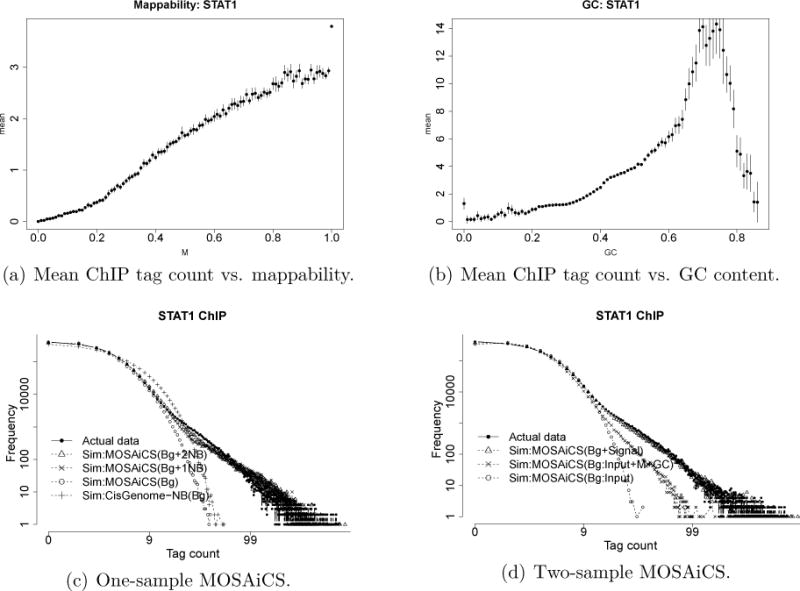
Mappability and GC content biases and goodness of fit for STAT1 ChIP-Seq sample. Panels (a) and (b) plot mean ChIP tag counts against the mappability score M_j and GC content GC_j, respectively. Panels (c) and (d) are the goodness of fit plots from one- and two-sample MOSAiCS models. Axes on both panels are in log10 scale. In panel (c), the background is fitted using M_j and GC_j. In panel (d), the background is fitted using M_j, GC_j, and X_j, or X_j only. Simulated data from estimated one-sample background model of CisGenome is displayed in panel (c).

Table 2.

Model selection based on BIC scores for the STAT1 ChIP sample

MOSAiCS	1S (1 NB)	1S (2 NB)	2S (Input Only)	2S (Input+M+GC)
BIC	3639751	3631390	3569584	3460109

NOTE: Each cell reports BIC score for one-sample (1S) and two-sample (2S) MOSAiCS.

A total of 104827, 18962, 47014, 116428, and 123143 peaks are obtained with MOSAiCS-1S, CisGenome-1S, MACS-1S (p-value threshold of 10⁻⁵), MACS-1S (p-value threshold of 10⁻²), and PeakSeq-1S with median sizes of 299 bp, 157 bp, 979 bp, 783 bp, and 217 bp, respectively. For all the one sample methods (except MACS which does not provide explicit FDR control), same nominal FDR level that corresponds to segment-wise nominal level of 0.05 for PeakSeq-1S is used as discussed in the previous section. Two-sample methods tend to identify smaller number of peaks (except for CisGenome) compared to their one-sample counterparts; however the median peaks sizes remain comparable to one-sample results (except for CisGenome). A total of 67426, 27642, 28458, and 97949 peaks with median peak sizes of 249 bp, 46 bp, 982 bp, and 287 bp are obtained by MOSAiCS-2S, CisGenome-2S, MACS-2S, and PeakSeq-2S. The same nominal FDR level from PeakSeq-1S is employed for CisGenome-2S and MOSAiCS-2S to enable direct comparisons to one-sample models. Results for PeakSeq-2S are obtained by filtering peaks identified by PeakSeq-1S using a second level nominal FDR of 0.05. Sample-swap scheme of MACS-2S results in a genome-wide estimated FDR level of 0.016. When we consider a similar FDR level for MOSAiCS-2S, the total number of peaks obtained is 57600 with a median peak size of 249 bp. In what follows, one-sample validation that relies on using naked DNA sample in a two-sample analysis is the only instance where the entire peak sets of the methods are utilized. The rest of the comparisons focus on top 5000 peaks of each method.

Since both mappability and GC content biases are attributes of the underlying naked DNA sequence in a ChIP-Seq experiment, a reasonable computational approach to validate peaks from one-sample analysis is to compare them with peaks obtained from a two-sample analysis of ChIP-Seq data using naked DNA as the control sample. To construct a gold-standard set of bound bins, we declare bins as bound in a two-sample analysis by a binomial test with p = D_C/(D_N + D_C), where D_C and D_N are the sequencing depths of ChIP and naked DNA samples, respectively (Ji et al., 2008). Table 3 reports bin level sensitivity and specificity, and peak level sensitivity of each method. For peak level sensitivity, we first define a gold-standard peak set over the bins that are declared bound in the two-sample analysis by merging contiguous bins within 200 bp of each other and filtering singleton bins. The performances of MOSAiCS-1S and PeakSeq-1S are comparable in terms of sensitivity both at the bin and peak levels and specificity. However, CisGenome-1S has lower sensitivity due to the over-estimation of the negative binomial background distribution as shown in Figure 5(c). In this comparison, we consider default MACS-1S cut-off of 10⁻⁵ as well as the larger 10⁻² cut-off that resulted in similar number of peaks to MOSAiCS-1S and PeakSeq-1S. Although increasing the threshold leads to higher sensitivity for MACS-1S without loss of specificity, MACS-1S overall has worse performance compared to MOSAiCS-1S and PeakSeq-1S. When we repeat this computational experiment by using peaks from a two-sample analysis with input DNA control as the gold standard set of peaks, the relative performances of the methods remain the same (Supplementary Materials Section 6.2).

Table 3.

Bin and peak level sensitivity and specificity for one-sample analysis of STAT1 ChIP-Seq data

STAT1 ChIP	MOSAiCS-1S	CS-1S	MACS-1S(1)	MACS-1S(2)	PS-1S
Sensitivity (peak)	0.901	0.256	0.657	0.811	0.949
Sensitivity (bin)	0.875	0.156	0.755	0.822	0.933
Specificity (bin)	0.993	0.999	0.988	0.964	0.992

NOTE: Sensitivity and specificity of different methods for one-sample analysis of STAT1 ChIP-Seq data are reported by assuming bound regions from a two-sample comparison with naked DNA to be the gold-standard set. MACS-1S(1) and MACS-1S(2) correspond to two different thresholds of p-value = 10⁻⁵ and p-value = 10⁻², respectively. CS-1S and PS-1S refer to CisGenome-1S and PeakSeq-1S, respectively.

We next perform motif analysis to elucidate differences among different sets of peaks and compare the two-sample analysis methods. If the peaks identified are indeed ChIP enriched regions, we should expect a large fraction of the peaks to contain one or more occurrences of the STAT1 motif and a decrease in the occurrence level with decreasing peak ranks. We scan ranked peaks of each method with the two STAT1 consensus binding sequences from the JASPAR database (Portales-Casamar et al., 2010). To avoid bias due to the variable peak widths identified by the different methods, we perform the motif analysis by fixing the peak widths (±150 bp of peak summit). For MACS and CisGenome, we use their estimated summit location. In MOSAiCS, the summit of a peak is defined as the midpoint of the bin with the largest ChIP tag count. Since PeakSeq does not provide summit information, it is excluded from this comparison. We also score each of these fixed width peaks using the FIMO tool of the MEME suite (Bailey and Elkan, 1994; Bailey et al., 2009). FIMO evaluates the significance of each subsequence under the STAT1 motif position weight matrix model and a background model. The motif analysis results using FIMO exhibit similar results as scanning peaks for the occurrences of the STAT1 consensus binding sequences. Hence, we present the results based on the consensus binding sequences. All the chromosomes are analyzed separately and results are summarized genome-wide. We report the proportion of peaks with a STAT1 motif in the top 5000 ordered peaks of each method in Figure 6(a). The observed pattern remains consistent for longer ranked peak lists and various width extensions around the summit. Overall, two-sample approaches have higher motif occurrence proportions compared to their one-sample counterparts. MOSAiCS-1S outperforms all the one-sample methods and MOSAiCS-2S (Input only) performs similar to CisGenome-2S. MOSAiCS-2S (Input+M+GC) outperforms all of the two-sample approaches.

Figure 6.

STAT1 motif analysis. (a) STAT1 consensus binding sequence occurrences across top 5000 peaks of each method. Peaks are rank ordered within each method. (b) –(c) Pairwise comparisons of peaks of MOSAiCS-1S and MOSAiCS-2S (Input+M+GC) with other one- and two-sample approaches. Barplots depict the proportion of peaks with the motif. Each three groups of bar plots corresponds to one pairwise comparison. “Common” refers to peaks common to both methods. Peaks unique to MOSAiCS are represented by the first barplot of each group and the peaks unique to the comparison method are represented as the middle barplot. (d) Mappability vs. GC content values of peaks that are (i) common between MOSAiCS-2S (Input+M+GC) and PeakSeq-2S (represented by “+”); (ii) unique to PeakSeq-TS (filled circle) and (iii) unique to MOSAiCS-2S (Input+M+GC) (filled triangle). Peaks with a STAT1 motif are depicted by open circles or triangles overlaying their solid versions.

We further explore this dataset to elucidate the differences among the peaks that are unique to each method. We compare peaks of MOSAiCS-1S and MOSAiCS-2S (Input+M+GC) to peaks from other methods in a pairwise manner. Figure 6(b) displays barplots of proportions of peaks with motif for peaks that are common between MOSAiCS-1S and other methods as well as for peaks that are unique to either MOSAiCS-1S or other methods. Figure 6(c) displays the same information for the two-sample comparisons. In these comparisons, peaks are again constrained to ±150 bp of their summit. Both analyses reveal that peaks unique to MOSAiCS have motif occurrence proportions higher than peaks unique to other approaches. Since PeakSeq is the only other method that explicitly utilizes the mappability concept, we compare peaks unique to MOSAiCS-2S (Input+M+GC) with peaks unique to PeakSeq-2S in Figure 6(d) by considering top 1000 peaks of each approach. In this comparison, original peaks of each method are utilized and the differences in peak widths are taken into account by controlling peak level FDR at 0.1 in the FIMO results (Supplementary Materials Section 6.3). Common peaks of the two approaches are provided as reference. Peaks with motif occurrences are depicted with open circles or triangles over the filled versions. This plot indicates that MOSAiCS-2S (Input+M+GC) is able to identify peaks with low mappability and/or low GC. In contrast, peaks unique to PeakSeq-2S tend to have higher mappability and higher GC content. Although top 1000 peaks are considered for display purposes, the observed pattern remains consistent for longer ranked peak lists.

We also compare peaks identified by each method with a small set of ChIP-chip target sites validated independently by qPCR (Euskirchen et al., 2007). Although we do not observe any striking diferences between the performances of different methods, MOSAiCS-1S and PeakSeq-1S perform better than CisGenome-1S and MACS-1S by capturing more true positive peaks, whereas CisGenome-2S performs slightly worse than the other two-sample methods (details are provided in Supplementary Materials). MOSAiCS and PeakSeq capture the highest number of true negatives in one- and two-sample comparisons.

4.2.2 GATA1 ChIP-Seq data

Similar to both the naked DNA and STAT1 ChIP-Seq data, GATA1 data from mouse exhibits both mappability and GC content biases (Supplementary Materials Figure 9). We compare the goodness of fit for MOSAiCS-1S and MOSAiCS-2S in Figures 7(a) and 7(b). Both the goodness of fit plots and BIC computations (Supplementary Materials Table 3) support a single negative binomial distribution for the signal component S_j of GATA1 ChIP-Seq data.

Figure 7.

GATA1 data analysis. Panels (a) and (b) are the goodness of fit plots from one- and two-sample MOSAiCS models. Axes on both panels are in log10 scale. In panel (a), the background is fitted using M_j and GC_j. In panel (b), the background is fitted using M_j, GC_j and X_j, or X_j only. (c) GATA1 consensus binding sequence occurrences in the top 3000 peaks of each method. Peaks are rank ordered within each method and peaks of different chromosomes are pooled for genome-wide representation. (d) Mappability vs. GC content values of peaks that are (i) common between MOSAiCS-2S (Input+M+GC) and MACS-2S (represented by “+”) ; (ii) unique to MACS-2S (filled circle), and (iii) unique to MOSAiCS-2S (Input+M+GC) (filled triangle). Peaks with a GATA1 consensus sequence are depicted by open circles or triangles overlaying their solid versions.

GATA-1 is one of the master regulators of blood cell development. A recent study on GATA1 (Zhang et al., 2009) showed that consensus sequence [A/T]GATA[A/G] is necessary for GATA1 binding but its occurrence alone does not guarantee binding of GATA1. Specifically, while more than 90% of GATA1-bound regions contain this motif, less than 1% of regions that contain the motif are actually bound by GATA1. Zhang et al. (2009) further showed that multiple occurrences of the consensus sequence [A/T]GATA[A/G] strongly discriminate GATA1-bound regions from unbound regions with the consensus, i.e., the average number of occurrences of [A/T]GATA[A/G] is about 2.3 in bound regions, compared to 1.1 in the unbound regions. Therefore, we scan each peak for two or more occurrences of the consensus sequence [A/T]GATA[A/G]. Additional results are provided in Section 7.3 of Supplementary Materials. Figure 7(c) displays proportion of peaks with two or more GATA1 motifs in the top 3000 ordered peaks of each method. The observed pattern remains consistent for different number of top peaks and various width extensions around the summit. MOSAiCS-2S (Input only) performs similar to MACS-2S and outperforms CisGenome-2S. MOSAiCS-2S (Input+M+GC) outperforms all the two-sample methods, whereas MOSAiCS-1S performs comparable to MOSAiCS-2S (Input+M+GC). Figure 7(d) displays mappability versus GC content of peaks that are unique to MOSAiCS-2S (Input+M+GC) and MACS-2S among the top 1000 peaks genome-wide (result are representative of other number of top peaks and peak widths are constrained to ±150 bp of the summit). Common peaks of the two approaches are provided as reference. Peaks with two or more occurrences of the GATA1 consensus sequence are depicted with an open circle or triangle over the filled versions. This plot indicates that peaks unique to MACS-2S tend to have higher mappability and GC content than peaks unique to MOSAiCS-2S (Input+M+GC).

5 Summary and discussion

We studied data from a naked DNA sequencing experiment and showed that count data from ChIP-Seq experiments exhibit mappability and GC content biases. We further illustrated that these biases may not be fully accounted for even in the presence of a matching input DNA control experiment. These observations led to a negative binomial regression model with mappability, GC content, and input DNA counts as covariates for background distribution of ChIP-Seq data. We then developed a mixture modeling framework named MOSAiCS which utilized this background model and captured the actual binding signal with additional negative binomial components. We showed that the flexible mixture model underlying MOSAiCS fits ChIP-Seq data from both human and mouse genome very well, and demonstrated that this model is able to achieve good operating characteristics based on motif analysis.

The hierarchical model underlying MOSAiCS offers a general framework that accommodates bin specific distributions and sequencing biases, and allows for information sharing across bins. Additionally, since the biases are incorporated in a regression framework, other factors, such as copy number variation in cancer cells which influence the generation of ChIP-Seq data could be incorporated.

The sequenced tags in the datasets presented here are ∼ 30 bp long. As a result, the mappability feature is computed using 30mers. 79.6% of the bases in human genome are mappable when using 30 bp in the definition of mappability (Rozowsky et al., 2009). Although this percentage increases with the ability to sequence longer tags, Rozowsky et al. (2009) reported that 89.3% of the genome is uniquely mappable by 70 bp tags. This indicates that mappability bias would be still highly relevant for longer tags. In fact, we have recently observed that mappability bias is still apparent for 75mer reads in a mouse ChIP-Seq dataset (Chung et al., 2011). In addition, all of the ChIP-Seq datasets submitted to GEO between February 2009 and July 2010 have tag length between 20 and 36 bp, indicating that the current state of the art for ChIP-Seq relies on short tags.

We presented data analysis results based on bin level FDR control. We recognize the inherent correlation structure of the observed data and refer interested reader to our work (Kuan et al., 2009) which incorporates the correlation structure via a hidden semi-Markov model (HSMM) and proposes a new meta approach for controlling FDR at peak level. Software implementing MOSAiCS is available at Bioconductor.

References

- Auerbach RK, Euskirchen G, Rozowsky J, Lamarre-Vincent N, Moqtaderi Z, Lefrançois P, Struhl K, Gerstein M, Snyder M. Mapping accessible chromatin regions using Sono-Seq. PNAS. 2009;106:14926–14931. doi: 10.1073/pnas.0905443106. [DOI] [PMC free article] [PubMed] [Google Scholar]
- Bachmann HS, Siffert W, Frey UH. Successful amplification of extremely GC-rich promoter regions using a novel ‘slowdown PCR’ technique. Pharmacogenetics. 2003;13:759–766. doi: 10.1097/00008571-200312000-00006. [DOI] [PubMed] [Google Scholar]
- Bailey T, Elkan C. Proceedings of the Second International Conference on Intelligent Systems for Molecular Biology. Menlo Park, California: AAAI Press; 1994. Fitting a mixture model by expectation maximization to discover motifs in biopolymers; pp. 28–36. http://meme.sdsc.edu/meme4_3_0/fimo-intro.html. [PubMed] [Google Scholar]
- Bailey TL, Boden M, Buske FA, Frith M, Grant CE, Clementi L, Ren J, Li WW, Noble WS. MEME Suite: tools for motif discovery and searching. Nucleic Acids Research. 2009;37:W202–W208. doi: 10.1093/nar/gkp335. [DOI] [PMC free article] [PubMed] [Google Scholar]
- Barski A, Cuddapah S, Cui K, Roh T, Schones D, Wang Z, Wei G, Chepelev I, Zhao K. High-resolution profiling of histone methylations in the human genome. Cell. 2007;129:823–837. doi: 10.1016/j.cell.2007.05.009. [DOI] [PubMed] [Google Scholar]
- Cawley S, Bekiranov S, Ng H, Kapranov P, Sekinger E, Kampa D, Piccolboni A, Sementchenko V, Cheng J, Williams A, Wheeler R, Wong B, Drenkow J, Yamanaka M, Patel S, Brubaker S, Tammana H, Helt G, Struhl K, Gingeras T. Unbiased mapping of transcription factor binding sites along human chromosomes 21 and 22 points to widespread regulation of non-coding RNAs. Cell. 2004;116:499–511. doi: 10.1016/s0092-8674(04)00127-8. [DOI] [PubMed] [Google Scholar]
- Cheng Y, Wu W, Kumar S, Yu D, Deng W, Tripic T, King D, Chen K, Zhang Y, Drautz D, Giardine B, Schuster S, Miller W, Chiaromonte F, Zhang Y, Blobel G, Weiss M, Hardison R. Erythroid GATA1 function revealed by genome-wide analysis of transcription factor occupancy, histone modifications, and mRNA expression. Genome Research. 2009;19:2172–2184. doi: 10.1101/gr.098921.109. [DOI] [PMC free article] [PubMed] [Google Scholar]
- Chung D, Kuan P, Li B, Sanalkumar R, Liang K, Bresnick E, Dewey C, Keleş S. Discovering transcription factor binding sites in highly repetitive regions of genomes with multi-read analysis of ChIP-Seq data. Technical Report No 1162, Department of Statistics, University, of Wisconsin-Madison. 2011 doi: 10.1371/journal.pcbi.1002111. [DOI] [PMC free article] [PubMed] [Google Scholar]
- Dempster AP, Laird N, Rubin D. Maximum likelihood from incomplete data via the EM algorithm. JRSSB. 1977;39:1–38. [Google Scholar]
- Dohm J, Lottaz C, Borodina T, Himmelbauer H. Substantial biases in ultra-short read data sets from high-throughput DNA sequencing. Nucleic Acids Research. 2008;36:e105. doi: 10.1093/nar/gkn425. [DOI] [PMC free article] [PubMed] [Google Scholar]
- Euskirchen G, Rozowsky J, Wei C, Lee W, Zhang Z, Hartman S, Emanuelsson O, Stolc V, Weissman S, Gerstein M, Ruan Y, Snyder M. Mapping of transcription factor binding regions in mammalian cells by ChIP: Comparison of array- and sequencing-based technologies. Genome Research. 2007;17:898–909. doi: 10.1101/gr.5583007. [DOI] [PMC free article] [PubMed] [Google Scholar]
- Ji H, Jiang H, Ma W, Johnson D, Myers R, Wong W. An integrated software system for analyzing ChIP-chip and ChIP-seq data. Nature Biotechnology. 2008;26:1293–1300. doi: 10.1038/nbt.1505. [DOI] [PMC free article] [PubMed] [Google Scholar]
- Johnson D, Mortazavi A, Myers R, Wold B. Genome-wide mapping of in vivo protein-DNA interactions. Science. 2007;316:1749–1502. doi: 10.1126/science.1141319. [DOI] [PubMed] [Google Scholar]
- Kuan P, Pan G, Thomson J, Stewart R, Keleş S. A hierarchical semi-Markov model for detecting enrichment with application to ChIP-Seq experiments. Technical Report No 1151, Department of Statistics, University of Wisconsin-Madison 2009 [Google Scholar]
- Kurdistani S, Tavazoie S, Grunstein M. Mapping global histone acetylation patterns to gene expression. Cell. 2004;117:721–733. doi: 10.1016/j.cell.2004.05.023. [DOI] [PubMed] [Google Scholar]
- Mikkelsen T, Ku M, Jaffe D, Issac B, Lieberman E, Giannoukos G, Alvarez P, Brockman W, Kim T, Koche RP, Lee W, Mendenhall E, O’Donovan A, Presser A, Russ C, Xie X, Meissner A, Wernig M, Jaenisch R, Nusbaum C, Lander E, Bernstein B. Genome-wide maps of chromatin state in pluripotent and lineage-committed cells. Nature. 2007;448:653–560. doi: 10.1038/nature06008. [DOI] [PMC free article] [PubMed] [Google Scholar]
- Newton M, Noueiry A, Sarkar D, Ahlquist P. Detecting differential gene expression with a semiparametric hierarchical mixture model. Biostatistics. 2004;5:155–176. doi: 10.1093/biostatistics/5.2.155. [DOI] [PubMed] [Google Scholar]
- Portales-Casamar E, Thongjuea S, Kwon AT, Arenillas D, Zhao X, Valen E, Yusuf D, Lenhard B, Wasserman WW, Sandelin A. JASPAR 2010: the greatly expanded open-access database of transcription factor binding profiles. Nucleic Acids Research. 2010;38:D105–10. doi: 10.1093/nar/gkp950. http://jaspar.cgb.ki.se/cgi-bin/jaspar_db.pl. [DOI] [PMC free article] [PubMed] [Google Scholar]
- Rozowsky J, Euskirchen G, Auerbach R, Zhang D, Gibson T, Bjornson R, Carriero N, Snyder M, Gerstein M. PeakSeq enables systematic scoring of ChIP-Seq experiments relative to controls. Nature Biotechnology. 2009;27:66–75. doi: 10.1038/nbt.1518. [DOI] [PMC free article] [PubMed] [Google Scholar]
- Seo Y, Chong H, Infante A, In S, Xie X, Osborne T. Genome-wide analysis of SREBP-1 binding in mouse liver chromatin reveals a preference for promoter proximal binding to a new motif. PNAS. 2009;106:13765–9. doi: 10.1073/pnas.0904246106. [DOI] [PMC free article] [PubMed] [Google Scholar]
- Valouev A, Ichikawa J, Tonthat T, Stuart J, Ranade S, Peckham H, Zeng K, Malek J, Costa G, McKernan K, Sidow A, Fire A, Johnson S. A high-resolution, nucleosome position map of C. elegans reveals a lack of universal sequence-dictated positioning. Genome Research. 2008;18:1051–1063. doi: 10.1101/gr.076463.108. [DOI] [PMC free article] [PubMed] [Google Scholar]
- Yuan G, Liu Y, Dion M, Slack M, Wu L, Altschuler S, Rando O. Genome-scale idenfication of nucleosome positions in S.cerevisiae. Science. 2005;309:626–630. doi: 10.1126/science.1112178. [DOI] [PubMed] [Google Scholar]
- Zhang X, Robertson G, Krzywinski M, Ning K, Droit A, Jones S, Gottardo R. PICS: Probabilistic inference for ChIP-Seq. Biometrics. 2010;67 doi: 10.1111/j.1541-0420.2010.01441.x. [DOI] [PubMed] [Google Scholar]
- Zhang Y, Liu T, Meyer C, Eeckhoute J, Johnson D, Bernstein B, Nussbaum C, Myers R, Brown M, Li W, Liu X. Model-based Analysis of ChIP-Seq (MACS) Genome Biology. 2008;9:R137. doi: 10.1186/gb-2008-9-9-r137. [DOI] [PMC free article] [PubMed] [Google Scholar]
- Zhang Y, Wu W, Cheng Y, King D, Harris R, Taylor J, Chiaromonte F, Hardison R. Primary sequence and epigenetic determinants of in vivo occupancy of genomic DNA by GATA1. Nucleic Acids Research. 2009;37:7024–7038. doi: 10.1093/nar/gkp747. [DOI] [PMC free article] [PubMed] [Google Scholar]
Associated Data
This section collects any data citations, data availability statements, or supplementary materials included in this article.