Comparison of SIRT and SQS for Regularized Weighted Least Squares Image Reconstruction

Abstract

Tomographic image reconstruction is often formulated as a regularized weighted least squares (RWLS) problem optimized by iterative algorithms that are either inherently algebraic or derived from a statistical point of view. This paper compares a modified version of SIRT (Simultaneous Iterative Reconstruction Technique), which is of the former type, with a version of SQS (Separable Quadratic Surrogates), which is of the latter type. We show that the two algorithms minimize the same criterion function using similar forms of preconditioned gradient descent. We present near-optimal relaxation for both based on eigenvalue bounds and include a heuristic extension for use with ordered subsets. We provide empirical evidence that SIRT and SQS converge at the same rate for all intents and purposes. For context, we compare their performance with an implementation of preconditioned conjugate gradient. The illustrative application is X-ray CT of luggage for aviation security.

I. Introduction

Iterative X-ray CT image reconstruction algorithms are often categorized as being either algebraic or statistical, with the former typically based on solving a system of equations centered around a forward model of the imaging process, and the latter based on maximizing a likelihood of the measurements. We are interested in the case where the two are related. For example, Sauer and Bouman [1] showed that a second-order Taylor-series expansion of a Poisson log-likelihood leads to a weighted least-squares (WLS) problem. Separable quadratic surrogate (SQS) methods for optimizing Poisson log-likelihoods also lead to WLS inner minimization problems [2], [3]. In these formulations the WLS weights have statistical meaning related to the modeled variance of the projection data. We show that statistical weighting is easily incorporated into algebraic algorithms such as SIRT (Simultaneous Iterative Reconstruction Technique) and SART (Simultaneous Algebraic Reconstruction Technique) [4].

The paper makes two main contributions. First, we establish similarity of a version of SIRT modified for WLS use with a version of the statistically based SQS algorithm. SIRT and SQS were shown previously to be similar in their basic unregularized forms [5], [6]. Here we show that they can solve the same Tikhonov regularized WLS problem using the same gradient descent approach, only with different diagonal preconditioners. Second, while SIRT is often relaxed by means of a user-defined step size [7], [8], SQS was not developed with relaxation in mind. We present a practical approach for selecting near-optimal step sizes for both algorithms. We extend the relaxation to apply also for ordered subsets (OS) which have become the de facto method for reducing the computational cost of iterative reconstruction in practice [9]. As part of this work, a scaling factor is introduced that accounts for potential imbalance among the subsets.

The SIRT and SQS algorithms considered are those commonly encountered in the current literature. For other versions of SIRT including the original algorithm and generalizations thereof, see [10]–[13]. A broad class of more contemporary SIRT-like algorithms can be found in [14]. Generalized versions of SQS are discussed in [2], [3]. We make no claims that the results presented in this paper apply to these alternative algorithms due to differences in their matrix set-up relative to ours. Comparison with the recently introduced acceleration of SQS based on Nesterov's momentum [15], which likely produces faster convergence than what is shown here, is likewise considered out-of-scope as a comparable version does not exist for SIRT. For context, we provide an empirical comparison with preconditioned conjugate gradient (PCG) which often converges quickly on well-behaved, unconstrained WLS problems.

The illustrative application is X-ray CT of luggage for aviation security for which imaging challenges include beam hardening and metal artifacts. Neither is explicitly addressed by the weighting and the regularization considered here although the effects of both are likely alleviated somewhat. We use the luggage data because the presence of dense objects and the noisy character of the data exacerbates any differences with respect to data-dependent convergence behavior for the algorithms compared.

II. Notation and Problem Definition

Let A = [a_ij] denote a non-negative m × n system matrix. Let W = diag{w_i} denote an m × m diagonal statistical weighting matrix with positive diagonal entries w_i. That is, we assume that rows for which w_i = 0 have been removed from A and W with corresponding columns removed from W as well. Defined in greater detail below, let Q denote an η × n regularization matrix where typically η ≥ n.

The general form of the regularized WLS (RWLS) image reconstruction problem addressed in this paper is

$${\mathit{x}}^{\ast }=\underset{\mathit{x}}{arg\; min}\mathrm{\Psi }(\mathit{x})$$ (1a)

$$\mathrm{\Psi }(\mathit{x})\triangleq \frac{1}{2}{\Vert \mathit{A}\mathit{x}-\mathit{y}\Vert }_{\mathit{W}}^2+\beta \frac{1}{2}{\Vert \mathit{Q}\mathit{x}\Vert }_2^2,$$ (1b)

where ${\Vert \mathit{u}\Vert }_{\mathit{W}}^2$ is shorthand for u′Wu, and x = [x_j] and y = [y_i] denote n × 1 and m × 1 vectors representing the unknown image and the log-normalized projection data, respectively. User-defined hyperparameter β establishes a trade-off between the data term (left norm) and the regularizer term (right norm).

Matrix Q is usually chosen to stress structural characteristics of x that are undesirable. We focus on two common regularizes, namely, minimum norm for which ${\Vert \mathit{Q}\mathit{x}\Vert }_2^2={\sum }_j{x}_j^2$, and first-order finite differences for which ${\Vert \mathit{Q}\mathit{x}\Vert }_2^2={\sum }_j{\sum }_{k\in {\mathcal{N}}_j}{(x_j-x_k)}^2$, where _j denotes the set of lexicographical predecessor neighbors. The former compensates for the linear system solved being ill-conditioned. The latter penalizes image roughness thereby implicitly encouraging smoothness. Adoption of other quadratic regularizers is trivial. We assume that Q and A have disjoint null spaces so that the cost function in (1) is strictly convex and has a unique minimizer [16].

Preconditioned gradient descent (PGD) solves RWLS problem (1) by means of the iterative update

$${\mathit{x}}^{(k+1)}={\mathit{x}}^{(k)}-\alpha \mathit{D}\nabla \mathrm{\Psi }({\mathit{x}}^{(k)})$$ (2)

where relaxation parameter α defines the step size, D is a preconditioning matrix, and k denotes iteration. Algebraic expansion reveals that PGD-RWLS is a Richardson Iteration for solving a linear system of equations; cf. [17] for definition and mathematical properties. That is,

$${\mathit{x}}^{(k+1)}={\mathit{x}}^{(k)}+\alpha \mathit{D}(\mathit{A}\prime \mathit{W}\mathit{y}-(\mathit{A}\prime \mathit{W}\mathit{A}+\beta \mathit{Q}\prime \mathit{Q}){\mathit{x}}^{(k)}).$$ (3)

Convergence is guaranteed for an arbitrary choice of initial estimate x⁽⁰⁾ if

$$0<\alpha <\frac{2}{{\lambda }_{max}},$$ (4)

with the fastest convergence rate obtained for

$${\alpha }^{\ast }=\frac{2}{{\lambda }_{max}+{\lambda }_{min}},$$ (5)

where λ_max and λ_min denote the largest and smallest eigenvalues of matrix D A′W A + βDQ′Q whose eigenvalues are all assumed to be strictly positive.

The remainder of the paper is devoted to derivation, analysis, and comparison of Richardson Iterations for SIRT and SQS that solve RWLS problem (1) using near-optimal α values. Well-established properties for eigenvalues are used extensively without reference, cf. [18], [19]. The shorthand notation M = M₁ + βM₂ where M₁ = D A′W A and M₂ = DQ′Q will be used for convenience. The smallest and largest eigenvalues of matrix M corresponding to the particular algorithm studied will be expressed as λ_min(M) and λ_max(M), with the explicit reference to M dropped when the matrix in question is obvious.

III. Method: SIRT-RWLS

A. Algorithm Derivation

Define the diagonal m × m and n × n matrices representing the inverse row and column sums of A, respectively, by R = diag{1/r_i} and C = diag{1/c_j}, where r_i = Σ_j a_ij, and c_j = Σ_i a_ij. We assume that the column sums c_j of A are positive, so by design C is positive definite. In other words, every pixel being reconstructed is intersected by one or more rays¹.

The classical SIRT iteration for “solving” Ax = y is

$${\mathit{x}}^{(k+1)}={\mathit{x}}^{(k)}+\alpha \mathit{C}\mathit{A}\prime \mathit{R}(\mathit{y}-{\mathit{A}\mathit{x}}^{(k)}).$$ (6)

This iteration is equivalent to gradient descent with diagonal preconditioner C of the “geometrically weighted” LS cost function $\frac{1}{2}{\Vert \mathit{A}\mathit{x}-\mathit{y}\Vert }_{\mathit{R}}^2$. Weighting by R means that minimization of the residual errors is per unit length, allowing rays that intersect larger portions of the field of view to tolerate larger errors than rays that intersect smaller portions. However, statistical weighting is preferable to geometric weighting for noisy data.

Adding the gradient of the regularizer to (6) leads to a version of SIRT that solves the following minimization problem [8]:

$${\mathit{x}}^{\ast }=\underset{\mathit{x}}{arg\; min}\frac{1}{2}{\Vert \mathit{A}\mathit{x}-\mathit{y}\Vert }_{\mathit{R}}^2+\beta \frac{1}{2}{\Vert \mathit{Q}\mathit{x}\Vert }_2^2.$$ (7)

Note use of an R-norm here. Next we modify SIRT using a simple variable transformation so that it solves RWLS problem (1) which is based on a W-norm. Let u ≜ Ax − y and ũ ≜ Mu. Choosing M ≜ W R⁻¹ implies that ${\Vert \mathit{u}\Vert }_{\mathit{W}}^2={\Vert \stackrel{\sim }{u}\Vert }_{\stackrel{\sim }{\mathit{R}}}^2$ where R̃ = M⁻¹R. More specifically, let à = [ã_ij] and ỹ = [ỹ_i], where ã_ij ≜ w_ir_ia_ij and ỹ_i ≜ w_ir_iy_i. Let the diagonal matrices corresponding to the row and column sums of à be R̃ ≜ diag {1/r̃_i} and C̃ ≜ diag {1/c̃_j} where ${\stackrel{\sim }{r}}_i\triangleq {\sum }_j{\stackrel{\sim }{a}}_{ij}=w_i{r}_i^2$ and c̃_j ≜ Σ_jã_ij. The SIRT-like iteration for “solving” Ãx = y with quadratic regularization is then obtained by left-multiplying the normal equations associated with the variable transformed version of (7) by C̃, followed by matrix splitting of the form C̃ Ã′R̃à = I – (I – C̃ Ã′R̃Ã). The resulting modified SIRT iteration is given by

$${\mathit{x}}^{(k+1)}=(\mathit{I}-\alpha \beta \stackrel{\sim }{\mathit{C}}\mathit{Q}\prime \mathit{Q}){\mathit{x}}^{(k)}+\alpha \stackrel{\sim }{\mathit{C}}\stackrel{\sim }{\mathit{A}}\prime \stackrel{\sim }{\mathit{R}}(\stackrel{\sim }{y}-\stackrel{\sim }{\mathit{A}}{\mathit{x}}^{(k)}).$$ (8)

The choice of α is discussed in the next two subsections, first for the unregularized case and then when regularization is applied.

Using the identities Ã′R̃ Ã = A′W A and Ã′R̃ỹ = A′W y, SIRT is expressed in terms of the original problem variables as follows:

$${\mathit{x}}^{(k+1)}=(\mathit{I}-\alpha \beta \stackrel{\sim }{\mathit{C}}\mathit{Q}\prime \mathit{Q}){\mathit{x}}^{(k)}+\alpha \stackrel{\sim }{\mathit{C}}\mathit{A}\prime \mathit{W}(\mathit{y}-{\mathit{A}\mathit{x}}^{(k)})={\mathit{x}}^{(k)}-\alpha \stackrel{\sim }{\mathit{C}}\nabla \mathrm{\Psi }({\mathit{x}}^{(k)}).$$ (9)

In other words, this modified SIRT algorithm is a Richardson Iteration that solves RWLS problem (1) using relaxed gradient descent with C̃ as a diagonal preconditioner. Note that

$${\stackrel{\sim }{c}}_j=\sum _i{\stackrel{\sim }{a}}_{ij}=\sum _i{a}_{ij}{w}_i{r}_i={[\mathit{A}\prime \mathit{W}\mathit{A}\mathbf{1}]}_j,$$ (10)

where 1 denotes a vector of n ones corresponding to the number of columns of A. Because C̃ merely serves as a preconditioner, it is amenable to substitution. Indeed, Section IV presents a SIRT-like derivation of the SQS algorithm for a different choice of C̃.

B. Step size for unregularized case

Assuming that A has full column rank and w_i > 0, then Ã′R̃ Ã = A′W A is symmetric positive definite. It therefore follows that C̃ Ã′R̃ Ã has strictly positive eigenvalues because it is similar to the symmetric positive definite matrix S A′W AS where S = C̃^1/2. Optimal step size α* given by (5) thus applies for unregularized SIRT. Obtaining values for λ_max and λ_min with respect to C̃ A′W A is addressed next. (See [20]–[22] for convergence analyses.)

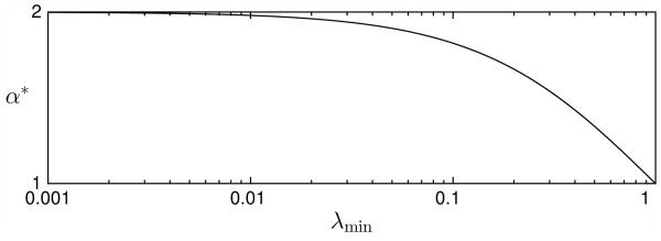
The spectral radius of a non-negative matrix is bounded by its smallest and largest row sums. Since C̃ Ã′ and R̃A are both non-negative and stochastic, so is their product C̃ Ã′R̃Ã = C̃ A′W A. The row sums of a stochastic matrix all equal 1. Therefore, λ_max = 1, which implies 1 ≤ α* ≜ 2/(1 + λ_min) < 2. Fig. 1 illustrates this relationship. Empirical comparisons of residual norms for typical 2D and 3D tomography problems have consistently shown that using α = 1.99 requires half as many iterations to achieve the same residual error as α = 1.00 [7]. This behavior indicates λ_min ≪ 1. While the value of λ_min is difficult to establish, we can find a conservative bound to use in its place. The trace of an n × n matrix equals the sum of its eigenvalues. The smallest eigenvalue can be no more than the average of all eigenvalues. Hence,

Fig. 1.

The value for optimal step size α* quickly approaches 2 as eigenvalue λ_min of C̃ A′ W A drops below 1.

$${\lambda }_{min}\le \frac{\text{tr}(\stackrel{\sim }{\mathit{C}}\mathit{A}\prime \mathit{W}\mathit{A})}{n}.$$ (11)

C. Step size for regularized case

We now examine selection of optimal step size α* for the regularized case. We use the fact that C̃(A′W A + βQ′Q) is similar to S(A′W A + βQ′Q)S where S remains defined as before. To simplify the notation, let M = M₁ + βM₂ where M₁ = S A′W AS and M₂ = SQ′QS. Note that M₁ and M₂ are both Hermitian matrices.

The sum of two positive semi-definite matrices is nonetheless positive definite, if they have different null spaces. This is the case for M₁ and M₂. Optimal step size α* thus remains given by (5) when regularization is applied. We must therefore determine the values of λ_max(M) and λ_min(M). As previously shown [8], this is easily done for minimum norm regularization where Q = I. However, for finite difference regularization where Q ≠ I, this is challenging. Instead, we derive bounds that lead to guaranteed convergence while keeping optimality in mind.

Applying Weyl's inequalities for the sum of Hermitian matrices:

$${\lambda }_{max}({\mathit{M}}_1)+\beta {\lambda }_{min}({\mathit{M}}_2)\le {\lambda }_{max}(\mathit{M})$$ (12a)

$$\le {\lambda }_{max}({\mathit{M}}_1)+\beta {\lambda }_{max}({\mathit{M}}_2)$$ (12b)

and

$${\lambda }_{min}({\mathit{M}}_1)+\beta {\lambda }_{min}({\mathit{M}}_2)\le {\lambda }_{min}(\mathit{M})$$ (13a)

$$\le {\lambda }_{min}({\mathit{M}}_1)+\beta {\lambda }_{max}({\mathit{M}}_2).$$ (13b)

SIRT converges to the RWLS minimizer x* if (4) holds. Using the upper bound on λ_max(M) given by (12) as well as the upper bound on λ_min(M) given by (13) would be valid but might be overly conservative. As an alternative, we combine the upper bound on the former with the lower bound on the latter to obtain a step size estimate that satisfies (4) and thus ensures convergence. That is,

$${\stackrel{\sim }{\alpha }}^{\ast }\triangleq \frac{2}{{\lambda }_{max}({\mathit{M}}_1)+{\lambda }_{min}({\mathit{M}}_1)+\beta ({\lambda }_{max}({\mathit{M}}_2)+{\lambda }_{min}({\mathit{M}}_2))}.$$ (14)

We analyze the similarity of α̃* to α* next by considering two extreme cases.

Case 1: Suppose λ_max(M) and λ_min(M) both take on their lower bounds. Then α̃* underestimates α* by the factor

$$\frac{{\stackrel{\sim }{\alpha }}^{\ast }}{{\alpha }^{\ast }}=\frac{{\lambda }_{max}({\mathit{M}}_1)+{\lambda }_{min}({\mathit{M}}_1)+2\beta {\lambda }_{min}({\mathit{M}}_2)}{{\lambda }_{max}({\mathit{M}}_1)+{\lambda }_{min}({\mathit{M}}_1)+\beta ({\lambda }_{max}({\mathit{M}}_2)+{\lambda }_{min}({\mathit{M}}_2))}.$$

We see that near-optimality is achieved when either of two conditions are met, namely, λ_min(M₂) ≈ λ_max(M₂) or βλ_max(M₂) ≪ λ_max(M₁). Sub-optimality results to a greater or lesser degree when neither of these conditions hold.

Case 2: Conversely, suppose λ_max(M) and λ_min(M) both take on their upper bounds. Then α̃* overestimates α* by the factor

$$\frac{{\stackrel{\sim }{\alpha }}^{\ast }}{{\alpha }^{\ast }}=\frac{{\lambda }_{max}({\mathit{M}}_1)+{\lambda }_{min}({\mathit{M}}_1)+2\beta {\lambda }_{max}({\mathit{M}}_2)}{{\lambda }_{max}({\mathit{M}}_1)+{\lambda }_{min}({\mathit{M}}_1)+\beta ({\lambda }_{max}({\mathit{M}}_2)+{\lambda }_{min}({\mathit{M}}_2))}.$$

Note that although α̃* may exceed α*, it is still a valid step size for SIRT. Near-optimality is again achieved when either of two conditions are met, this time λ_min(M₂) ≈ λ_max(M₂) or 2βλ_max(M₂) ≪ λ_max(M₁). Sub-optimality results to a greater or lesser degree when neither of these conditions hold.

Restating (14) in terms of the original problem variables we get

$${\stackrel{\sim }{\alpha }}^{\ast }=\frac{2}{\mathrm{\Lambda }(\stackrel{\sim }{\mathit{C}}\mathit{A}\prime \mathit{W}\mathit{A})+\beta \mathrm{\Lambda }(\stackrel{\sim }{\mathit{C}}\mathit{Q}\prime \mathit{Q})}$$ (15)

Where

$$\begin{array}{c}\mathrm{\Lambda }(\stackrel{\sim }{\mathit{C}}\mathit{A}\prime \mathit{W}\mathit{A})\triangleq 1+{\lambda }_{min}(\stackrel{\sim }{\mathit{C}}\mathit{A}\prime \mathit{W}\mathit{A})\\ \mathrm{\Lambda }(\stackrel{\sim }{\mathit{C}}\mathit{Q}\prime \mathit{Q})\triangleq {\lambda }_{max}(\stackrel{\sim }{\mathit{C}}\mathit{Q}\prime \mathit{Q})+{\lambda }_{min}(\stackrel{\sim }{\mathit{C}}\mathit{Q}\prime \mathit{Q}).\end{array}$$

Whether applied to 2D or 3D reconstruction, minimum norm regularization yields

$${\lambda }_{max}(\stackrel{\sim }{\mathit{C}}\mathit{Q}\prime \mathit{Q})={\lambda }_{max}(\stackrel{\sim }{\mathit{C}})=1/min{\stackrel{\sim }{c}}_j$$ (16a)

$${\lambda }_{min}(\stackrel{\sim }{\mathit{C}}\mathit{Q}\prime \mathit{Q})={\lambda }_{min}(\stackrel{\sim }{\mathit{C}})=1/max{\stackrel{\sim }{c}}_j.$$ (16b)

For finite difference regularization, we first note that a multiplicative equivalent to Weyl's inequalities follows from the relation between (maximum) eigenvalues and matrix norms, namely,

$${\lambda }_{max}(\stackrel{\sim }{\mathit{C}}\mathit{Q}\prime \mathit{Q})\le {\lambda }_{max}(\stackrel{\sim }{\mathit{C}}){\lambda }_{max}(\mathit{Q}\prime \mathit{Q})\le {\lambda }_{max}(\stackrel{\sim }{\mathit{C}}){\Vert \mathit{Q}\prime \mathit{Q}\Vert }_1,$$

where ‖Q′Q‖₁ denotes the maximum absolute column sum. In 2D, for a first-order neighborhood a typical row of Q′Q has one entry valued 4 and four entries valued −1, leading to ‖Q′Q‖₁ = 8, In 3D, one entry is valued 6 and six entries are valued −1, leading to ‖Q′Q‖₁ = 12. Extending to other neighborhoods is trivial. Combined with singularity of Q′Q carrying through to C̃Q′Q, we thus have that

$${\lambda }_{max}(\stackrel{\sim }{\mathit{C}}\mathit{Q}\prime \mathit{Q})\le \frac{4N}{{min}_j{\stackrel{\sim }{c}}_j}$$ (17a)

$${\lambda }_{min}(\stackrel{\sim }{\mathit{C}}\mathit{Q}\prime \mathit{Q})=0$$ (17b)

where N is 2 or 3 corresponding to the problem dimensionality.

To summarize, RWLS image reconstruction by means of SIRT as given by (9) is carried out by applying weighting to the system matrix and the log-normalized data. Near-optimal step size α* is obtained by substituting (16) or (17) into (15) and using (11). That is,

$${\stackrel{\sim }{\alpha }}^{\ast }=\frac{2}{1+\frac{\text{tr}(\stackrel{\sim }{\mathit{C}}\mathit{A}\prime \mathit{W}\mathit{A})}{n}+\beta (\frac{{\upsilon }_1}{{min}_j{\stackrel{\sim }{c}}_j}+\frac{{\upsilon }_2}{{max}_j{\stackrel{\sim }{c}}_j})},$$ (18)

where ν₁ = ν₂ = 1 for minimum-norm regularization and ν₁ = 4N and ν₂ = 0 for N-dimensional finite difference regularization. Computing the trace term requires the equivalent effort of one combined forward and back-projection.

IV. Method: SQS-RWLS

A. Algorithm Derivation

Although SQS was presented originally for non-quadratic log-likelihoods like the Poisson model [2], it is equally applicable to RWLS problems like (1) [15], [23], where W is the reciprocal of the (modeled) variance of y_i. The SQS approach to solving such problems traditionally has been derived using surrogate functions [2], [23], based on the work of De Pierro [24], [25]. Here we present a different “SIRT-like” derivation for the RWLS case that leads to near-optimal relaxation.

The idea is to first specify an appropriate system of equations of the form Bx = d such that applying the classical SIRT algorithm (6) to that system solves RWLS problem (1) and then add relaxation. As noted earlier, classical SIRT solves a geometrically weighted LS problem rather than the statistical WLS problem, so it requires a judicious choice of B and d to coerce SIRT into working as desired here.

We first use variable transforms akin to those used in (8) to rewrite RWLS cost function (1) in a stacked form, namely,

$$\mathrm{\Psi }(\mathit{x})=\frac{1}{2}{\Vert \mathit{B}\mathit{x}-\mathit{d}\Vert }_{\widehat{\mathit{R}}}^2,$$ (19)

Where

$$\mathit{B}\triangleq \left[\begin{array}{c}\stackrel{\sim }{\mathit{A}}\\ \beta \widehat{\mathit{Q}}\end{array}\right],\mathit{d}\triangleq \left[\begin{array}{c}\stackrel{\sim }{\mathit{y}}\\ \mathbf{0}\end{array}\right],\widehat{\mathit{R}}\triangleq \left[\begin{array}{cc}\stackrel{\sim }{\mathit{R}}& \mathbf{0}\\ \mathbf{0}& (1/\beta ){\mathit{P}}^2\end{array}\right]$$

and Q̂ = P⁻¹Q, P ≜ diag {1/p_k}, p_k ≜ Σ_j |q_kj|, and 0 denotes, as appropriate, a vector of zeros whose length is the number of rows of Q or matrices of zeros whose dimensions correspond to the number of rows and columns of R̃ and P.

The generalization of SIRT to extend beyond non-negative matrices by using such absolute sums has been published previously [20], [26]. That generalization is needed here because Q has negative elements for finite difference regularizers. It is easily shown that R̂ = diag {1/r̂_i} where the absolute row sums of B are r̂_i = Σ_j |b_ij|. Denoting the absolute column sums via Ĉ = diag {1/ĉ_j} where ĉ_j = Σ_i|b_ij|, the classic SIRT method for “solving” Bx = d is given by

$${\mathit{x}}^{(k+1)}={\mathit{x}}^{(k)}+\widehat{\mathit{C}}{\mathit{B}}^{\text{'}}\widehat{\mathit{R}}(\mathit{d}-\mathit{B}{\mathit{x}}^{(k)}).$$

Using the identities B′ R̂B = A′W A + βQ′ Q and B′ R̂d = A′W y, we can express this iteration using the original problem variables while also introducing relaxation:

$${\mathit{x}}^{(k+1)}=(\mathit{I}-\alpha \beta \widehat{\mathit{C}}{\mathit{Q}}^{\text{'}}\mathit{Q}){\mathit{x}}^{(k)}+\alpha \widehat{\mathit{C}}{\mathit{A}}^{\text{'}}\mathit{W}(\mathit{y}-\mathit{A}{\mathit{x}}^{(k)})={\mathit{x}}^{(k)}-\alpha \widehat{\mathit{C}}\nabla \mathrm{\Psi }({\mathit{x}}^{(k)}).$$ (20)

Remarkably, iteration (20) with α = 1 is exactly the usual SQS iteration (cf. [23, eqn. (17)]) for minimizing RWLS problem (1). The convergence proof for SQS is normally based on the fact it decreases Ψ(x^(k)) monotonically [27]. One can also see that convergence follows from the fact that λ_max(ĈB′ R̂B) = λ_max(Ĉ(A′W A + βQ′ Q)) ≤ 1 by arguments similar to those in [7, eqn.(6)].

We see that the SQS version of SIRT in (20) is also preconditioned gradient descent. The “denominator” elements of preconditioner Ĉ are given by

$${\widehat{c}}_j=\sum _i|b_{ij}|={[{\mathit{A}}^{\text{'}}\mathit{W}\mathit{A}\mathbf{1}]}_j+\beta \sum _k|q_{kj}|p_k.$$ (21)

For 2D and 3D minimum norm regularization, use of Q = I implies that p_k = 1 and Σ_k|q_kj| p_k = 1 leading to ĉ_j = c̃_j + β. For first-order finite difference regularization, each row of Q has at most one entry valued 1 and one entry valued −1 such that p_k ≤ 2. In 2D, each column of Q has at most two entries valued 1 and two entries valued −1 while in 3D there are at most three of each. Thus, Σ_k|q_kj|p_k ≤ 4N leading to ĉ_j ≤ c̃_j + 4Nβ where N again refers to the problem dimensionality. For the experimental results presented in Section VI, we used a simple implementation based on ĉ_j = c̃_j + 4Nβ. This choice is exact for periodic boundary conditions and is a value upper bound otherwise.

To summarize, SIRT-RWLS iteration (9) and SQS-RWLS iteration (20) are identical for solving RWLS problem (1), except that SIRT uses C̃ and SQS uses Ĉ to precondition the relaxed gradient descent.

B. Step size for unregularized case

Without regularization, SIRT-WLS and SQS-WLS are identical. The latter can thus be relaxed using the same method developed for the former in Section III which typically results in α* = 1.99.

C. Step size for regularized case

When regularization is applied, the optimal step size is given by

$${\widehat{\alpha }}^{\ast }=\frac{2}{\mathrm{\Lambda }(\widehat{\mathit{C}}{\mathit{A}}^{\text{'}}\mathit{W}\mathit{A})+\beta \mathrm{\Lambda }(\widehat{\mathit{C}}{\mathit{Q}}^{\text{'}}\mathit{Q})}$$ (22)

Where

$$\mathrm{\Lambda }(\widehat{\mathit{C}}{\mathit{A}}^{\text{'}}\mathit{W}\mathit{A})\triangleq {\lambda }_{max}(\widehat{\mathit{C}}{\mathit{A}}^{\text{'}}\mathit{W}\mathit{A})+{\lambda }_{min}(\widehat{\mathit{C}}{\mathit{A}}^{\text{'}}\mathit{W}\mathit{A})\mathrm{\Lambda }(\widehat{\mathit{C}}{\mathit{Q}}^{\text{'}}\mathit{Q})\triangleq {\lambda }_{max}(\widehat{\mathit{C}}{\mathit{Q}}^{\text{'}}\mathit{Q})+{\lambda }_{min}(\widehat{\mathit{C}}{\mathit{Q}}^{\text{'}}\mathit{Q}).$$

We develop the needed eigenvalue bounds next.

With respect to Λ(ĈA′WA), we apply the transformation Ĉ = ŜC̃ where Ŝ ≜ diag {ŝ_j} and ŝ_j ≜ c̃_j/ĉ_j to write λ_max(ĈA′WA) = λ_max(ŜC̃A′WA) ≤ λ_max(Ŝ). We thus have that,

$$\mathrm{\Lambda }(\widehat{\mathit{C}}{\mathit{A}}^{\text{'}}\mathit{W}\mathit{A})\le {\widehat{s}}_{max}+{\lambda }_{min}(\widehat{\mathit{C}}{\mathit{A}}^{\text{'}}\mathit{W}\mathit{A})$$

where ŝ_max ≜ max_j ŝ_j and

$${\lambda }_{min}(\widehat{\mathit{C}}{\mathit{A}}^{\text{'}}\mathit{W}\mathit{A})\le \frac{\text{tr}(\widehat{\mathit{C}}{\mathit{A}}^{\text{'}}\mathit{W}\mathit{A})}{n}.$$

The bounds for Λ(ĈQ′ Q) are established using derivations from the previous section. For minimum norm regularization,

$${\lambda }_{max}(\widehat{\mathit{C}}{\mathit{Q}}^{\text{'}}\mathit{Q})={\lambda }_{max}(\widehat{\mathit{C}})=1/min{\widehat{\mathit{C}}}_j$$ (23a)

$${\lambda }_{min}(\widehat{\mathit{C}}{\mathit{Q}}^{\text{'}}\mathit{Q})={\lambda }_{min}(\widehat{\mathit{C}})=1/max{\widehat{\mathit{C}}}_j$$ (23b)

while for finite difference regularization,

$${\lambda }_{max}(\widehat{\mathit{C}}{\mathit{Q}}^{\text{'}}\mathit{Q})\le \frac{4N}{{min}_j{\widehat{c}}_j}$$ (24a)

$${\lambda }_{min}(\widehat{\mathit{C}}{\mathit{Q}}^{\text{'}}\mathit{Q})=0.$$ (24b)

Combining the above, we obtain the following near-optimal step size α* expression:

$${\widehat{\alpha }}^{\ast }=\frac{2}{{\widehat{s}}_{max}+\frac{\text{tr}(\widehat{\mathit{C}}{\mathit{A}}^{\text{'}}\mathit{W}\mathit{A})}{n}+\beta (\frac{w_1}{{min}_j{\widehat{c}}_j}+\frac{w_2}{{max}_j{\widehat{c}}_j})},$$ (25)

where w₁ = w₂ = 1 for minimum-norm regularization and w₁ = 4N and w₂ = 0 for N-dimensional finite difference regularization.

The similarity of step size expressions (18) for SIRT-RWLS and (25) for SQS-RWLS is striking. Which of the two algorithms has the fastest convergence rate depends on the relation between α̃*C̃ and α̂*Ĉ since these terms constitute the only difference between them. Note that α̃*C̃ ≈ α̂*Ĉ when c̃_j ≫ w₁β since ĉ_j = c̃_j + w₁β. We expect this mild condition to be met for most applications.

V. Ordered subsets

Typically SIRT and SQS establish the low-frequency components of an image faster than the high-frequency components. Ordered subsets (OS) is a well-known, albeit heuristic technique for accelerating convergence in early iterations [9]. The idea is to partition the projection data and the corresponding system matrix rows and successively perform updates using these subsets. To simplify the development of OS-SIRT below, we assume partitioning is done in such a way that each subset includes a view of all pixels².

Although quite distinct from one another when originally presented, the terms SIRT [10] and SART [28] are now used interchangeably in the literature. SIRT updates the image using all projections whereas SART uses one projection at a time. In that sense, SART can be viewed as an OS version of SIRT where each subset consists of a single projection. Variants thereof where multiple projections are grouped to form subsets have been studied for both algorithms, e.g., [29], [30].

In this paper, we use the ordered subsets approach taken for SQS [23]. Each full iteration uses the gradients of M partial cost functions of the form

$${\mathrm{\Psi }}_m(\mathit{x})\triangleq \frac{1}{2}{\Vert {\mathit{A}}_m\mathit{x}-{\mathit{y}}_m\Vert }_{{\mathbf{W}}_m}^2+\beta \frac{1}{2M}{\Vert \mathit{Q}\mathit{x}\Vert }_2^2$$

where the m-subscripts indicate that only data for the mth subset is used. Letting k = nM + m denote the mth sub-iteration of the nth full-iteration, the relaxed, preconditioned (incremental) gradient descent algorithms considered can be written as

$${\mathit{x}}^{(\frac{k+1}{M})}={\mathit{x}}^{(\frac{k}{M})}-\alpha \mathit{D}M\nabla {\mathrm{\Psi }}_m({\mathit{x}}^{(\frac{k}{M})})$$ (26)

where OS-SIRT and OS-SQS correspond to αD = α̃*C̃ and αD = α̂*Ĉ, respectively. The preconditioners are not altered as a result of the subsets.

In practice, the subset balance condition ∇Ψ(x) ≈ M∇Ψ_m(x) will hold only approximately and the iterates approach a limit cycle rather than converging to a minimizer. When the subset imbalance is mild but non-negligible, OS-SIRT and OS-SQS may exhibit sub-optimal convergence rates due to step size estimates α̃* and α̂* being too aggressive. To compensate, we introduce a scaling factor that reduces the step size based on a measure of the imbalance. Specifically, we quantify and use the degree to which the term $M\mathrm{\Lambda }(\mathit{D}{\mathit{A}}_m^{\text{'}}{\mathit{W}}_m{\mathit{A}}_m)$ associated with (26) deviates from Λ(DA′W A) which plays a central role in the step size computations.

Consider (temporarily) computing subset specific step size estimates based on matrices for the individual subsets. That is,

$${\alpha }_m^{\ast }=\frac{2}{M\mathrm{\Lambda }(\mathit{D}{\mathit{A}}_m^{\text{'}}{\mathit{W}}_m{\mathit{A}}_m)+\beta \mathrm{\Lambda }(\mathit{D}{\mathit{Q}}^{\text{'}}\mathit{Q})}$$ (27)

where $\mathrm{\Lambda }(\mathit{D}{\mathit{A}}_m^{\text{'}}{\mathit{W}}_m{\mathit{A}}_m)$ is the only unknown entity.

In a manner similar to when developing relaxation for SQS-RWLS, let D = S_mC_m where ${\mathit{S}}_m\triangleq \text{diag}\left\{s_j^m\right\}$ and $s_j^m\triangleq c_j^m/d_j$. Furthermore, let ${\mathit{C}}_m\triangleq \text{diag}\left\{c_j^m\right\}$ where $c_j^m$ denotes column sums of A_m akin to (10). Then ${\lambda }_{max}(\mathit{D}{\mathit{A}}_m^{\text{'}}{\mathit{W}}_m{\mathit{A}}_m)={\lambda }_{max}({\mathit{S}}_m{\mathit{C}}_m{\mathit{A}}_m^{\text{'}}{\mathit{W}}_m{\mathit{A}}_m)\le s_{max}^m$ where $s_{max}^m\triangleq {max}_j{s}_j^m$. Also, ${\lambda }_{min}(\mathit{D}{\mathit{A}}_m^{\text{'}}{\mathit{W}}_m{\mathit{A}}_m)\le s_{max}^m{\lambda }_{min}({\mathit{C}}_m{\mathit{A}}_m^{\text{'}}{\mathit{W}}_m{\mathit{A}}_m)$. Rather than introducing a trace based bound for the right hand side eigenvalue, we use the approximation ${\lambda }_{min}({\mathit{C}}_m{\mathit{A}}_m^{\text{'}}{\mathit{W}}_m{\mathit{A}}_m)\approx {\lambda }_{min}(\mathit{C}{\mathit{A}}^{\text{'}}\mathit{W}\mathit{A})$. These considerations, along with the definition of $S_M\triangleq {max}_m{s}_{max}^{m}M$ to eliminate the subset dependency, lead us to define the following generic OS-PGD step size estimate

$${\alpha }_{\text{os}}^{\ast }=\frac{2}{S_M\mathrm{\Lambda }(\mathit{D}{\mathit{A}}^{\text{'}}\mathit{W}\mathit{A})+\beta \mathrm{\Lambda }(\mathit{D}{\mathit{Q}}^{\text{'}}\mathit{Q})}.$$ (28)

For OS-SIRT, replacing D by C̃ results in the step size estimate

$${\stackrel{\sim }{\alpha }}_{\text{os}}^{\ast }=\frac{2}{{\stackrel{\sim }{\mathit{S}}}_M\mathrm{\Lambda }(\stackrel{\sim }{\mathit{C}}{\mathit{A}}^{\text{'}}\mathit{W}\mathit{A})+\beta \mathrm{\Lambda }(\stackrel{\sim }{\mathit{C}}{\mathit{Q}}^{\text{'}}\mathit{Q})}.$$ (29)

where ${\stackrel{\sim }{S}}_M\triangleq {max}_m{max}_j({\stackrel{\sim }{c}}_j^m/{\stackrel{\sim }{c}}_j)M$.

For OS-SQS, replacing D by Ĉ results in the step size estimate

$${\widehat{\alpha }}_{\text{os}}^{\ast }=\frac{2}{{\widehat{\mathit{S}}}_M\mathrm{\Lambda }(\widehat{\mathit{C}}{\mathit{A}}^{\text{'}}\mathit{W}\mathit{A})+\beta \mathrm{\Lambda }(\widehat{\mathit{C}}{\mathit{Q}}^{\text{'}}\mathit{Q})}.$$ (30)

where ${\widehat{S}}_M\triangleq {max}_m{max}_j({\widehat{c}}_j^m/{\widehat{c}}_j)M$.

When the subsets are well-balanced, S_M ≈ 1 and the step size is comparable to the one developed before considering ordered subsets. When the subsets are mildly imbalanced, the use of S_M results in a smaller value for the step size. For large enough M, the subsets will be imbalanced to the point where neither OS-SIRT nor OS-SQS will come sufficiently close to x*. The only viable remedy for this case is to use fewer subsets.

We close this section by reminding the reader that ordered subsets do not guarantee convergence, unless one gradually decreases the relaxation parameter [31]. The proposed rescaling of the step sizes for OS-SIRT and OS-SQS is equally heuristic. We neither claim that the rescaling results in convergent algorithms nor do we claim that convergence will not occur in practice without it. The most important contribution of the above developments is perhaps scaling factor S_M and its use for indicating subset imbalance.

VI. Experimental Results

A. Comparing SIRT and SQS

We implemented SIRT-RWLS and SQS-RWLS as described above and empirically compared their convergence rates. The data consisted of luggage scans obtained as part of a U.S. Department of Homeland Security sponsored project managed by ALERT at Northeastern University (Boston, MA) [32]. Several suitcase-like containers were scanned using an Imatron C300 fifth-generation electron-beam X-ray CT scanner. We used two of these data sets denoted DS1 and DS2. After data rebinning, the system was modeled as a third-generation equiangular fan-beam geometry having a circular source trajectory covering 216 degrees over 864 view angles that were 0.25 degrees apart and 864 detectors spanning a range of 41.3 degrees corresponding to a pitch of approximately 0.048 degrees. The source-to-isocenter distance was 675 mm while the isocenter-to-detector distance was 900 mm yielding 2.33 × magnification. Polynomial beam hardening correction was applied. We reconstructed 512 × 512 images using isotropic 0.928 mm wide pixels. Pixels outside a circular support region having radius 475 mm were excluded from consideration. Modeled on area intersection the resulting 746,496 × 204,836 system matrix A contained approximately one billion non-zero elements. Weight matrix W was formed by partly reversing the log-normalization of the projection data, i.e., w_i = exp(−y_i). The beam intensity was unknown and assumed constant which may be inaccurate.

SIRT and SQS were both initialized using filtered back-projection for x⁽⁰⁾. We ran 256 iterations of each algorithm for each experiment. Comparisons were based on values of Ψ(x^(k)). We performed OS reconstructions for M = 1, 2, 4, 8, 16, and 32. Non-negativity was imposed on the image after each subiteration using gradient projection. Reconstructions were computed for a wide range of β values. We report results for β = 1.0 as that value produced images that were clearly regularized but not overly so.

Figures 2 and 3 show β = 1.0 and β = 5.0 reconstructions respectively for DS1 using SIRT and minimum norm regularization and DS2 using SQS and finite difference regularization. The intensity values represent modified Hounsfield units (MHU) for which air has a value of 0 while water has a value of 1000. The images were cropped to 350 × 430 to save space. DS1 is corrupted by a metal streak artifact that cuts into the water container. DS2 suffers even more from both metal streak and metal shading artifacts. These types of corruptions are not uncommon for luggage data although the particular data used here was purposely chosen to be challenging. More importantly, the images produced by SIRT and SQS are indistinguishable from one another. For the minimum norm regularized images of DS1, the numerical difference is within ±0.01 MHU. For the finite difference regularized images of DS2, the numerical difference is within ±0.10 MHU. Similar results were obtained for DS1 using finite difference regularization and DS2 using minimum norm regularization.

Fig. 2.

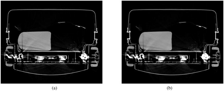
DS1 reconstructions using minimum norm regularization: (a) SIRT-RWLS using β = 1.0 and (b) SIRT-RWLS using β = 5.0. Image intensity levels truncated to 0-1800 MHU.

Fig. 3.

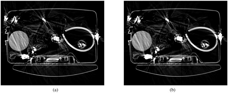
DS2 reconstructions using finite difference regularization: (a) SQS-RWLS using β = 1.0 and (b) SQS-RWLS using β = 5.0. Image intensity levels truncated to 0-1800 MHU.

Table I lists minimum and maximum column sum values for C̃ as used by SIRT to compute LS and WLS solutions. Data weighting is seen to lower especially the minimum values. With the maximum values remaining large, α̃* ≈ α̂*. Due to the minimum values being lowered quite substantially, Ĉ ≤ C̃ meaning some pixels will be updated more slowly by SQS than by SIRT. The degree to which that creates a difference in convergence rates is studied below.

Table I. SIRT Column Sum Statistics.

	Both-LS	DS1-WLS	DS2-WLS
maxj c̃j	666,140	412,423	321,432
minj c̃j	304,479	3,941	1,026

Table II provides eigenvalue bounds for the data and regularizer terms associated with SIRT reconstruction based on minimum norm (MN) and finite difference (FD) regularization for SIRT. Table III provides the similar numbers for SQS. The largest eigenvalue of the data term equals 1 for SIRT by design and approximately does so for SQS because ŝ_max = max c̃_j/ĉ_j ≈ 1. We can therefore infer that the conservative upper bound used for the smallest eigenvalue of the data term in both cases is at least three orders of magnitude smaller than the largest eigenvalue indicating SIRT and SQS are tasked with solving very poorly conditioned problems. We also see that the eigenvalue bounds for the regularizer terms are substantially smaller than those for the data terms.

Table II. SIRT Eigenvalue Bounds.

Data	Reg.	Λ(C̃ A′ W A)	Λ(C̃Q′Q)
DS1	MN	1.000903	0.000256
DS1	FD	1.000903	0.002030
DS2	MN	1.000933	0.000977
DS2	FD	1.000933	0.007794

Table III. SQS Eigenvalue Bounds.

Data	Reg.	Λ(Ĉ A′ W A)	Λ(ĈQ′Q)
DS1	MN	1.000901	0.000256
DS1	FD	1.000884	0.002026
DS2	MN	1.000930	0.000976
DS2	FD	1.000908	0.007733

The above observations indicate that near-optimal step size values, i.e., α ≈ 2/(1 + ε), should be achievable. Tables IV and V list the actual step sizes computed for OS-SIRT and OS-SQS along with the S̃_M and Ŝ_M scaling factors. For M = 1, near-optimal step sizes were indeed produced for both SIRT and SQS. Increasingly smaller step sizes resulted for larger values of M due to data dependent subset imbalances becoming more significant. SIRT and SQS behaved the same in this regard.

Table IV.

OS-SIRT Step Size α̃* as Function of M.

	DS1 (MN)		DS2 (FD)
M	S̃M	α̃*	S̃M	α̃*
1	1.0000	1.9977	1.0000	1.9977
2	1.0094	1.9792	1.0094	1.9792
4	1.0263	1.9466	1.0262	1.9467
8	1.0525	1.8982	1.0524	1.8983
16	1.1240	1.7776	1.1239	1.7777
32	1.3654	1.4636	1.3653	1.4636

Table V.

OS-SQS Step Size α̂* as Function of M.

	DS1 (MN)		DS2 (FD)
M	ŜM	α̂*	ŜM	α̂*
1	1.0000	1.9827	1.0000	1.9829
2	1.0053	1.9723	1.0052	1.9727
4	1.0158	1.9520	1.0154	1.9530
8	1.0433	1.9011	1.0428	1.9021
16	1.1106	1.7868	1.1103	1.7874
32	1.2859	1.5449	1.2854	1.5456

We computed step size estimates for non-regularized WLS reconstructions and found them to be comparable to those listed in Tables IV and V. Regularization thus had negligible impact on α̃* and α̂*. We also computed step size estimates for pure LS reconstructions. These were all closer to 2 than the RWLS estimates but did decrease for larger value of M. This does not indicate a problem with the system model. Rather, it is related to physical characteristics of the system geometry, such as the rays being much wider at one end than at the other, causing pixel coverage to be both location and view dependent. Combined with a shortscan source trajectory, the larger angular strides associated with larger values of M invariably induce subset column sum differences. This in turn results in a larger value of the S_M scaling factor which causes the step size estimate to decrease.

While all OS-SIRT and OS-SQS configurations were found to be convergent, Ψ(x^(k)) values for M = 16 and 32 were larger than those for M = 8 indicating convergence to a limit cycle. We suspect the reason for this behavior is related to the aforementioned data variations. The statistical weighting considered in this paper is not intended to handle such systematic data inconsistencies.

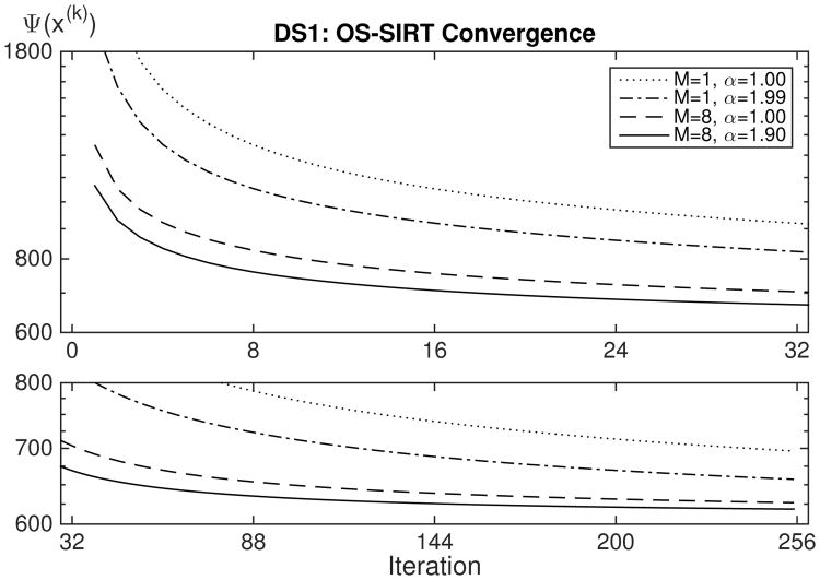
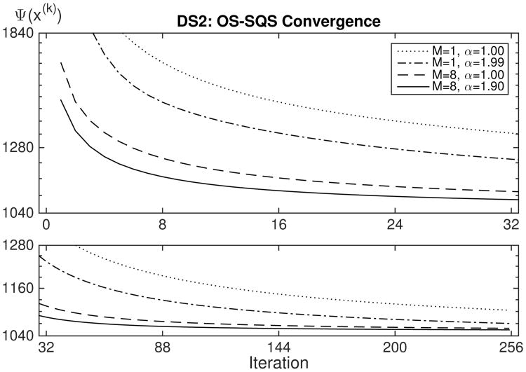
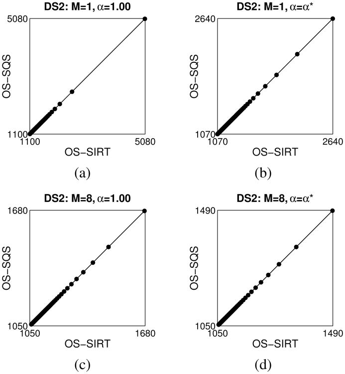
Figures 4 and 5 show Ψ(x^(k)) for OS-SIRT applied to DS1 and OS-SQS applied to DS2, respectively, using M = 1 and M = 8 as well α = 1.00 and α = α*. The axes are scaled to best show configuration differences. This includes the x-axes being linear and the y-axes logarithmic. The plots for M ≤ 8 show similar convergence behavior, while the plots for M ≥ 16 confirm the previously mentioned fast convergence to a sub-optimal Ψ value. Data set DS1 is noisy but cleaner and thus likely more internally consistent than DS2. This is reflected in the final Ψ value for DS1 being substantially lower than that of DS2.

Fig. 4.

Cost function Ψ(x^(k)) plots for application of OS-SIRT to data set DS1 using minimum norm regularization.

Fig. 5.

Cost function Ψ(x^(k)) plots for application of OS-SQS to data set DS2 using finite difference regularization.

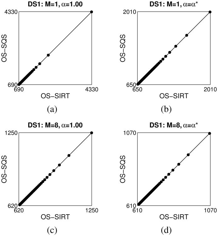
Figures 6 and 7 provide scatter plots of OS-SIRT versus OS-SQS for the combinations of M and α mentioned above. A correlation coefficient of 1.00 was computed for all plots indicating that applying OS-SQS to DS1 and OS-SIRT to DS2 would produce identical plots to those shown in Figs. 4 and 5.

Fig. 6.

Scatter plots of OS-SIRT versus OS-SQS for DS1 reconstructions using minimum norm regularization.

Fig. 7.

Scatter plots of OS-SIRT versus OS-SQS for DS2 reconstructions using finite difference regularization.

There is in other words, no difference between the convergence rates of SIRT and SQS for the data tested

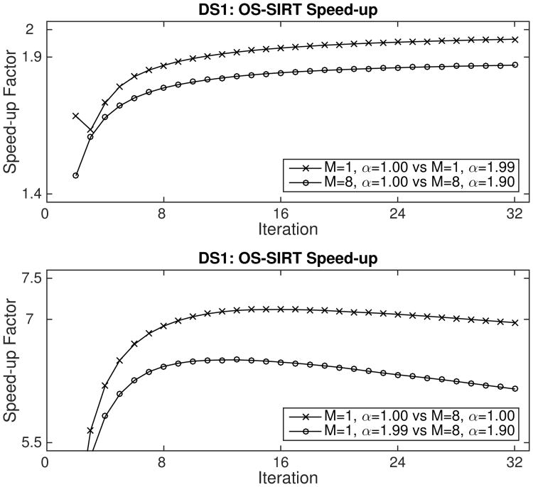
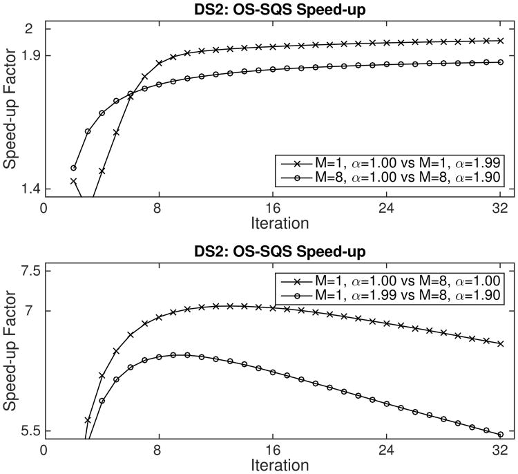
To more clearly illustrate the speed-up produced by relaxation, Figs. 8 and 9 plot the ratio of the interpolated number of iterations of the slower curve relative to the number of iterations needed to reach the same value of the faster curve. The two top plots show that the relaxed versions of OS-SIRT and OS-SQS decrease Ψ close to α̃* and α̂* times faster than when using α = 1.00 for the first 32 iterations for which speed-up factors were computed. This speed-up clearly indicates that the proposed step size estimates for SIRT, namely, (18) and (29), and SQS, namely, (25) and (30), are very effective. The two bottom plots reconfirm that subset imbalances cause both OS-SIRT and OS-SQS to quickly approach a near-final value of Ψ whereafter only slow progress is made in reducing it. Ideally, the speed-up would be constant at 8 corresponding to the number of subsets used.

Fig. 8.

OS-SIRT speed-up factors for data set DS1 using minimum norm regularization. Top: α = 1 versus α = α*. Bottom: M = 1 versus M = 8.

Fig. 9.

OS-SQS speed-up factors for data set DS2 using finite difference regularization. Top: α = 1 versus α = α*. Bottom: M = 1 versus M = 8.

B. Comparison with Conjugate Gradient

SIRT-RWLS and SQS-RWLS are stationary iterative methods that repeatedly apply a gradient based “correction” to the current estimate of the solution. As shown above, convergence is governed by the largest and smallest eigenvalues of the underlying iteration matrix. Conjugate gradient (CG), on the other hand, is a Krylov subspace method [17] that iteratively forms an increasingly larger basis for which an approximation to the solution is found that minimizes the cost function in that subspace. Convergence depends on the full eigenvalue spectrum and is proportional to the square root of the number of iterations needed by SIRT [14]. Preconditioning (PCG) may accelerate the convergence rate further.

To compare the behavior of the proposed relaxed versions of SIRT and SQS with PCG when applied to RWLS problem (1), we implemented the Polak-Ribiére CG algorithm along with a Jacobi preconditioner [33], [34]. Enforcing non-negativity on the solution was not considered as such a constraint is difficult to efficiently incorporate into a CG algorithm due to the need for conjugacy preservation among the basis vectors, c.f. [35]. All algorithms were regularized using β = 1.0. OS-SIRT and OS-SQS were executed for M = 8.

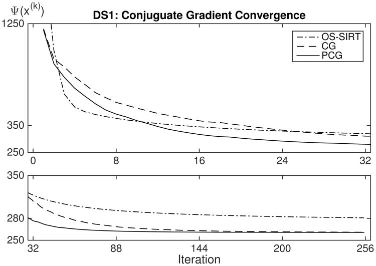
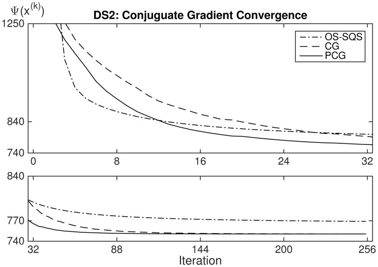
Figure 10 shows PCG-RWLS reconstructions for DS1 using minimum norm regularization and DS2 using finite difference regularization. The corresponding SIRT-RWLS and SQS-RWLS reconstructions look similar to those in Figs. 2 and 3. The difference images reveal that high density objects and edges exhibit the greatest degree of disparity. As indicated by Figs. 11 and 12, cost function Ψ(x^(k)) has converged to a lower value for PCG-RWLS than for SIRT-RWLS and SQS-RWLS. While the images of the former kind thus are “more optimal” than those of the latter, one could argue that they are qualitatively less desirable due to their noisier appearance and the Gibbs-like ringing which can be seen to accentuate object edges as well as the metal streak artifacts.

Fig. 10.

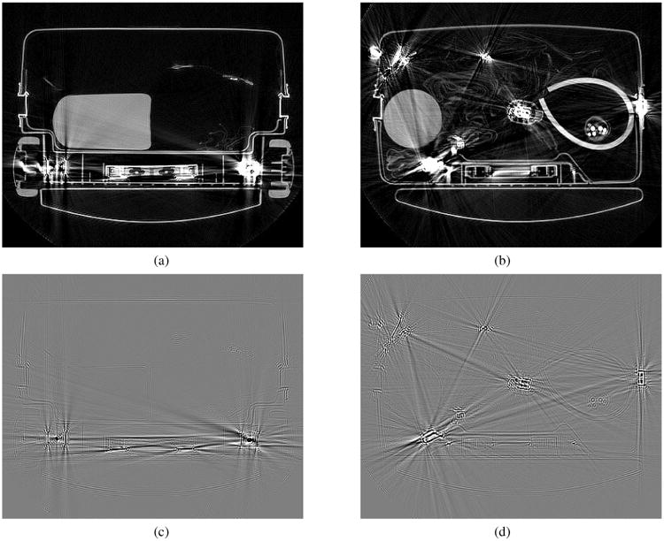
PCG-RWLS reconstructions: (a) DS1 using minimum norm regularization, (b) DS2 using finite difference regularization, (c) DS1 difference between PCG-RWLS and SIRT-RWLS and (d) DS2 difference between PCG-RWLS and SQS-RWLS. Image intensity levels truncated to 0-1800 MHU for (a) and (b). Difference image intensity levels truncated to ±1000 MHU for (c) and (d).

Fig. 11.

Cost function Ψ(x^(k)) plots for application of OS-SIRT, CG and PCG to data set DS1 using minimum norm regularization.

Fig. 12.

Cost function Ψ(x^(k)) plots for application of OS-SQS, CG and PCG to data set DS2 using finite difference regularization.

Figures 11 and 12 show that OS-SIRT and OS-SQS converge faster than both CG and PCG during the early iterations, only to be overtaken when limit cycle behavior sets in. CG is seen to converge more slowly than PCG, but eventually reaches the same limit value due to data inconsistencies causing PCG to stall out. The cost function limit values are lower than those in Figs. 4 and 5 due to non-negativity not being enforced.

For reconstructions based on 256 iterations, a speed-up factor of 16 should be expected. After the first 32 iterations when limit cycle behavior has not yet become an issue, OS-SIRT and OS-SQS are seen to have converged to about the same value of Ψ(x^(k)) as the CG algorithm. This correlates with the speed-up factors of 2 and 8 shown to be achieved for the proposed near-optimal relaxation and the use of eight ordered subsets. For cleaner data, OS-SIRT and OS-SQS could be run for more subsets in which case they would converge faster than shown here, possibly to the point where they converge as fast as the PCG algorithm. While the convergence rate for PCG could be improved using a more sophisticated preconditioner, the design and implementation thereof is by no means easy. Combined with their ability to effortlessly incorporate non-negativity, OS-SIRT and OS-SQS thus appear to form viable alternatives to PCG for solving RWLS problems.

VII. Conclusion

We have shown that SIRT can be modified to solve a true WLS problem, i.e., without the otherwise inherent geometric weighting. We have also shown that such a version of SIRT and a commonly used version of SQS solve the same Tikhonov regularized WLS problem using the same gradient descent approach except for their (diagonal) preconditioning and step size. We developed practical methods for selecting the step sizes for both algorithms. Empirical results suggest these step sizes to achieve near-optimal relaxation across a wide range of data. We proposed a heuristic adjustment to the step size estimates that accounts for imbalances when using ordered subsets. The convergence rates for SIRT and SQS were found to be indistinguishable.

We compared the proposed relaxed OS-SIRT and OS-SQS algorithms with an implementation of PCG. Non-negativity was not applied due to associated implementation complications for PCG. We found OS-SIRT and OS-SQS to converge faster than PCG during the early iterations. However, OS-SIRT and OS-SQS eventually succumbed to limit cycle behavior due to data inconsistencies, resulting in PCG achieving a lower final value of the cost function. A qualitative comparison of the associated images did not support a lower cost function value corresponding to a more desirable image. OS-SIRT and OS-SQS thus appear to form viable alternatives to PCG for solving RWLS problems.

While SIRT cannot be extended to handle non-quadratic regularizers, SQS was designed with these in mind. Compelling future work includes the possibility of introducing relaxation of such an extension. Comparison with acceleration based on Nesterov's momentum [15] would be interesting in that context.

Biographies

Jens Gregor received the M.S.E.E. degree from Aalborg University, Aalborg, Denmark, in 1988, and earned a Ph.D. degree in electrical engineering in 1991, also from Aalborg University. He has worked at the University of Tennessee, Knoxville, since then. He is now a Professor in the Department of Electrical Engineering and Computer Science as well as an Adjunct Associate Professor of Radiology. His research interests are in pattern recognition and computational aspects of image reconstruction.

Jeffrey A. Fessler received the B.S.E.E. degree from Purdue University in 1985, the M.S.E.E. degree from Stanford University in 1986, and the M.S. degree in Statistics from Stanford University in 1989. From 1985 to 1988 he was a National Science Foundation Graduate Fellow at Stanford, where he earned a Ph.D. degree in electrical engineering in 1990. He has worked at the University of Michigan since then. From 1991 to 1992 he was a Department of Energy Alexander Hollaender Post-Doctoral Fellow in the Division of Nuclear Medicine. From 1993 to 1995 he was an Assistant Professor in Nuclear Medicine and the Bioengineering Program. He is now a Professor in the Departments of Electrical Engineering and Computer Science, Radiology, and Biomedical Engineering. He became a Fellow of the IEEE in 2006, for contributions to the theory and practice of image reconstruction. He received the Francois Erbsmann award for his IPMI93 presentation, and the Edward Hoffman Medical Imaging Scientist Award in 2013. He has served as an associate editor for IEEE Transactions on Medical Imaging, the IEEE Signal Processing Letters, and the IEEE Transactions on Image Processing, and is currently serving as an associate editor for the IEEE Transactions on Computational Imaging. He has chaired the IEEE T-MI Steering Committee and the ISBI Steering Committee. He was co-chair of the 1997 SPIE conference on Image Reconstruction and Restoration, technical program co-chair of the 2002 IEEE International Symposium on Biomedical Imaging (ISBI), and general chair of ISBI 2007. His research interests are in statistical aspects of imaging problems.

References

- 1.Sauer K, Bouman C. A local update strategy for iterative reconstruction from projections. IEEE Trans Signal Proc. 1993;41:534–548. [Google Scholar]
- 2.Erdogan H, Fessler JA. Ordered subsets algorithms for transmission tomography. Physics in Medicine and Biology. 1999;44:2835–2851. doi: 10.1088/0031-9155/44/11/311. [DOI] [PubMed] [Google Scholar]
- 3.Elbakri IA, Fessler JA. Statistical image reconstruction for polyenergetic x-ray computed tomography. IEEE Trans Medical Imaging. 2002;21:89–99. doi: 10.1109/42.993128. [DOI] [PubMed] [Google Scholar]
- 4.Kak A, Slaney M. Principles of CT Imaging. SIAM; 2001. [Google Scholar]
- 5.Shi D, Zou Y, Zamyatin AA. Weighted simultaneous algebraic econstruction technique. Proc Intl Mtg on Fully 3D Image Recon in Rad and Nuc Med. 2011:160–2. [Google Scholar]
- 6.Shi D. Unified interpretations of variants of simultaneous algebraic reconstruction technique (SART) Proc Intl Mtg on Fully 3D Image Recon in Rad and Nuc Med. 2013:166–8. [Google Scholar]
- 7.Gregor J, Benson T. Computational analysis and improvement of SIRT. IEEE Trans Medical Imaging. 2008;27:918–924. doi: 10.1109/TMI.2008.923696. [DOI] [PubMed] [Google Scholar]
- 8.Gregor J. Algorithmic improvements to SIRT with application to X-ray CT of luggage. Proc 3rd Intl Mtg on Image Formation in X-ray CT. 2014:121–4. [Google Scholar]
- 9.Hudson HM, Larkin RS. Accelerated image reconstruction using ordered subsets of projection data. IEEE Trans Medical Imaging. 1994;13:601–609. doi: 10.1109/42.363108. [DOI] [PubMed] [Google Scholar]
- 10.Gilbert P. Iterative methods for the three-dimensional reconstruction of an object from projections. Journal of Theoretical Biology. 1972;36:105–117. doi: 10.1016/0022-5193(72)90180-4. [DOI] [PubMed] [Google Scholar]
- 11.Herman G, Lent A. Iterative reconstruction algorithms. Comput Biol Med. 1976;6:273–294. doi: 10.1016/0010-4825(76)90066-4. [DOI] [PubMed] [Google Scholar]
- 12.Herman G, Lent A. Quadratic optimization for image reconstruction I. Computer Graphics and Image Processing. 1976;5:319–332. [Google Scholar]
- 13.Lakshminarayanan A, Lent A. Methods of least squares and SIRT in reconstruction. Journal of Theoretical Biology. 1979;76:267–295. doi: 10.1016/0022-5193(79)90313-8. [DOI] [PubMed] [Google Scholar]
- 14.van der Sluis A, van der Horst HA. SIRT and CG-type methods for the iterative solution of sparse linear least-squares problems. Linear Algebra and its Applications. 1990;130:257–302. [Google Scholar]
- 15.Kim D, Ramani S, Fessler HA. Combining ordered subsets and momentum for accelerated X-ray CT image reconstruction. IEEE Trans Medical Imaging. 2015 doi: 10.1109/TMI.2014.2350962. To appear. [DOI] [PMC free article] [PubMed] [Google Scholar]
- 16.Delaney AH, Bresler Y. Globally convergent edge-preserving regularized reconstruction: an application to limited-angle tomography. IEEE Trans Image Processing. 1998;7:204–221. doi: 10.1109/83.660997. [DOI] [PubMed] [Google Scholar]
- 17.Saad Y. Iterative Methods for Sparse Linear Systems. PWS Publishing Co; Boston: 1996. [Google Scholar]
- 18.Horn R, Johnson C. Matrix Analysis. Cambridge Univ. Press; 1985. [Google Scholar]
- 19.Golub G, van Loan C. Matrix Computations. Johns Hopkins Univ. Press; 1996. [Google Scholar]
- 20.Jiang M, Wang G. Convergence of the simultaneous algebraic reconstruction technique (SART) IEEE Trans Image Processing. 2003;12:957–961. doi: 10.1109/TIP.2003.815295. [DOI] [PubMed] [Google Scholar]
- 21.Jiang M, Wang G. Convergence studies on iterative algorithms for image reconstruction. IEEE Trans Medical Imaging. 2003;22:569–579. doi: 10.1109/TMI.2003.812253. [DOI] [PubMed] [Google Scholar]
- 22.Wang J, Zheng Y. On the convergence of generalized simultaneous iterative reconstruction algorithms. IEEE Trans Image Processing. 2007;16:1–6. doi: 10.1109/tip.2006.887725. [DOI] [PubMed] [Google Scholar]
- 23.Kim D, Pal D, Thibault JB, Fessler JA. Accelerating ordered subsets image reconstruction for X-ray CT using spatially non-uniform optimization transfer. IEEE Trans Medical Imaging. 2013;32:1965–1978. doi: 10.1109/TMI.2013.2266898. [DOI] [PMC free article] [PubMed] [Google Scholar]
- 24.De Pierro AR. On the relation between the ISRA and the EM algorithm for positron emission tomography. IEEE Trans Medical Imaging. 1993;12:328–333. doi: 10.1109/42.232263. [DOI] [PubMed] [Google Scholar]
- 25.De Pierro AR. A modified expectation maximization algorithm for penalized likelihood estimation in emission tomography. IEEE Trans Medical Imaging. 1995;14:132–137. doi: 10.1109/42.370409. [DOI] [PubMed] [Google Scholar]
- 26.Censor Y, Elfving T. Block-iterative algorithms with diagonally scaled oblique projections for the linear feasibility problem. SIAM J Matrix Anal Appl. 2002;24:40–58. [Google Scholar]
- 27.Jacobson MW, Fessler JA. An expanded theoretical treatment of iteration-dependent majorize-minimize algorithms. IEEE Trans Image Processing. 2007;16:2411–2422. doi: 10.1109/tip.2007.904387. [DOI] [PMC free article] [PubMed] [Google Scholar]
- 28.Andersen AH, Kak AC. Simultaneous algebraic reconstruction technique (SART): A superior implementation of the ART algorithm. Ultrasonic Imaging. 1984;6:81–94. doi: 10.1177/016173468400600107. [DOI] [PubMed] [Google Scholar]
- 29.Wang G, Jiang M. Ordered-subset simultaneous algebraic reconstruction technique (OS-SART) Journal of X-ray Science & Technology. 2004;12:169–177. [Google Scholar]
- 30.Benson T, Gregor J. Distributed iterative image reconstruction for micro-CT with ordered-subsets and focus of attention problem reduction. Journal of X-ray Science & Technology. 2004;12:231–240. [Google Scholar]
- 31.Ahn S, Fessler JA. Globally convergent image reconstruction for emission tomography using relaxed ordered subsets algorithms. IEEE Trans Medical Imaging. 2003;22:613–626. doi: 10.1109/TMI.2003.812251. [DOI] [PubMed] [Google Scholar]
- 32.http://www.northeastern.edu/alert/transitioning-technology/alert-datasets
- 33.Press W, Teukolsky S, Vetterling W, Flannery B. Numerical Recipes. Cambridge Univ. Press; 2007. [Google Scholar]
- 34.Fessler JA, Booth SD. Conjugate-gradient preconditioning methods for shift-variant PET image reconstruction. IEEE Trans Image Processing. 1999;8:688–699. doi: 10.1109/83.760336. [DOI] [PubMed] [Google Scholar]
- 35.Gregor J, Rannou F. SPIE Medical Imaging Conf. Vol. 4322. San Diego, CA: 2001. Least squares framework for projection MRI reconstruction; pp. 888–898. [Google Scholar]