Biocellion: accelerating computer simulation of multicellular biological system models

Abstract

Motivation: Biological system behaviors are often the outcome of complex interactions among a large number of cells and their biotic and abiotic environment. Computational biologists attempt to understand, predict and manipulate biological system behavior through mathematical modeling and computer simulation. Discrete agent-based modeling (in combination with high-resolution grids to model the extracellular environment) is a popular approach for building biological system models. However, the computational complexity of this approach forces computational biologists to resort to coarser resolution approaches to simulate large biological systems. High-performance parallel computers have the potential to address the computing challenge, but writing efficient software for parallel computers is difficult and time-consuming.

Results: We have developed Biocellion, a high-performance software framework, to solve this computing challenge using parallel computers. To support a wide range of multicellular biological system models, Biocellion asks users to provide their model specifics by filling the function body of pre-defined model routines. Using Biocellion, modelers without parallel computing expertise can efficiently exploit parallel computers with less effort than writing sequential programs from scratch. We simulate cell sorting, microbial patterning and a bacterial system in soil aggregate as case studies.

Availability and implementation: Biocellion runs on x86 compatible systems with the 64 bit Linux operating system and is freely available for academic use. Visit http://biocellion.com for additional information.

Contact: seunghwa.kang@pnnl.gov

1 INTRODUCTION

Cells interact with other cells by moving, adhering, dividing and secreting and receiving diffusible molecules. As a result, unicellular organisms are able to form communities with complex macroscopic structure and behavior (e.g. biofilm), while multicellular organisms, where cells can differentiate to perform different functions, form tissues. Multicellular biological systems respond to external stimuli and reshape the surrounding environment. Complex interactions among cells and their biotic and abiotic environment drive multicellular system behavior. Understanding the impact of such interactions is a critical step in our ability to predict and manipulate important biological system behaviors in the areas of energy (Melnicki et al., 2013), environment (Daly, 2000) and health care (Weinberg, 2007).

Computational biologists have started to investigate multicellular biological systems via modeling and simulation. Cells and their biotic and abiotic environment constitute a biological system. Computational biologists commonly model the environment by imposing a grid on the extracellular space. There are two principal approaches in modeling cells: population-based modeling and discrete agent-based modeling. Population-based modeling (Anderson and Chaplain, 1998; Xavier et al., 2009) approximates the cells within any grid box by a set of variables associated with the grid box. Discrete agent-based modeling (Anderson and Chaplain, 1998; Ferrer et al., 2008; Jeannin-Girardon et al., 2013) maps each cell (or subcellular element) to a discrete simulation entity.

Biologists have accumulated a significant amount of knowledge about cell and subcellular organelle behaviors. Discrete agent-based modeling naturally translates the accumulated knowledge to a mathematical model. However, the computational complexity of discrete agent-based modeling increases proportional to the number of discrete agents. Many biological systems contain 1 million to 100 billion cells (Byrne and Drasdo, 2009). Researchers have acknowledged the necessity of supercomputers and a proper parallel implementation to simulate millions to billions of cells within a reasonable time (Jiao and Torquato, 2011). The lack of ‘a proper parallel implementation’ forces computational biologists to simply use a small number of cells (which does not reflect the reality), resort to population-based modeling or develop a hybrid approach that uses discrete agent-based modeling for a fraction of the cells [e.g. invading cancer cells (Frieboes et al., 2010)] and adopts population-based modeling for the remaining cells.

The most practical approach to build a high fidelity model of important biological systems is starting from a relatively simple model and incrementally improving the model fidelity, which typically results in increases in the complexity and scale of the model. For this approach to be successful, we believe that an incremental increase in model complexity and scale should require only an incremental amount of additional programming effort. Population-based modeling and the hybrid approach are inherently limited in this regard. Averaging a heterogeneous population of cells to a few variables associated with a grid box cannot model cell granularity events in the required level of detail (McDougall et al., 2002). Adopting the hybrid approach, fewer and fewer cells can be modeled using the population-based approach as modelers adopt more complex mathematics to describe individual cell behaviors.

We designed Biocellion to allow computational biologists to use discrete agent-based modeling—in combination with high-resolution grids to model the extracellular environment—from simple small-scale models to highly complex large-scale models with millions to billions of cells. We aim to address the increase in computational complexity exploiting high-performance computing (HPC): adoption of efficient algorithms, careful performance tuning and exploitation of parallel computers ranging from multicore PCs to Cloud computers and supercomputers.

Parallel computers are abundant but developing efficient software for large parallel computers is a highly demanding task (Bernholdt, 2007) and becoming even more so with new multicore processors and manycore accelerators such as Intel Xeon Phi and NVIDIA graphics processing units (Kang et al., 2011). Biological system models are diverse and even a model from a single research group changes significantly over a relatively short period. This imposes a challenge in software reusability, which is problematic considering the high development cost of parallel software. Biocellion asks users to express their model specifics by filling the function body of pre-defined model routines. Biocellion executes and evaluates the user-provided model routines in parallel using efficient solvers. This approach provides Biocellion users having no HPC expertise with the flexibility needed to support a variety of models and the performance required to simulate large systems.

1.1 Related work

VirtualCell (Loew and Schaff, 2001) and Smoldyn (Andrews, 2012) simulates one or a small number of cells in detail—modeling cell membrane and subcellular structures in high spatial resolution or individually modeling every molecule. CompuCell3D (Izaguirre et al., 2004) and Morpheus (Starruß et al., 2014) adopt the Cellular Potts model (Graner and Glazier, 1992) and target biological systems with up to millions of cells. The Cellular Potts Model partitions the simulation domain into equally sized cubic boxes and maps a set of boxes to each cell. The Cellular Potts Model evaluates the overall biological system energy based on mathematical constraints derived from cell behavioral rules and dynamically updates the mapping between boxes and cells to minimize the overall system energy. However, Voss-Böhme (2012) claims that modeling biological system behaviors using the contrived energy term complicates interpreting simulation output. Discrete agent-based modeling maps a cell to an agent (or multiple agents). Discrete agents can be placed anywhere in the simulation domain to within the limits of floating point precision. Discrete agents move and change sizes to model cell movement and growth. There are multiple general-purpose software frameworks supporting agent-based modeling—e.g. FLAME (Chin et al., 2012) and SWARM (Minar et al., 1996). These tools are highly flexible in modeling agent behaviors but require more programming efforts than software frameworks specifically designed for biological system modeling; modelers need to implement partial differential equation (PDE) solvers from scratch to update molecular concentrations by solving PDEs. iDynoMiCS (Lardon et al., 2011) is an agent-based simulation framework designed for biofilm modeling targeting non-programmers. iDynoMiCS does not support parallel computing. To the best of our knowledge, Biocellion is the only software framework that is specifically designed for discrete agent-based simulation of general multiscale multicellular biological system models and exploits high-performance parallel computing to simulate millions to billions of cells.

2 METHODS

2.1 Biocellion design motivation

Mathematical models of biological systems are diverse, but at the same time, many of the models share common programming and computational challenges. For example, enumerating cell pairs close enough to interact via direct contact is a recurring task. PDE is commonly used to model spatio-temporal variation of molecular concentrations in the extracellular environment. Efficient PDE solvers can be reused. Every parallel simulation of multicellular models must distribute the work of simulating (i) cells, (ii) cell–cell interactions and (iii) different subregions of the extracellular space across compute cores on multiple compute nodes. These are recurring tasks.

A biological system model needs to integrate multiple biological processes occurring in different timescales to simulate the system in its entirety. This requires multiple time step sizes. Solving PDEs to model molecular diffusion often requires a much smaller time step size than simulating cell movement due to cell growth and cell–cell shoving and adhesion. Biological processes are interrelated. The required coupling interval—the maximum time step size to simulate one biological process, ignoring the changes due to another biological process, without introducing a significant simulation artifact—varies widely for different pairs of biological processes. Multiple time step sizes and coupling intervals complicate data exchange patterns in parallel computing.

The HPC community has developed efficient (but complex to implement) algorithms for many of these recurring issues [e.g. developing efficient PDE solvers (Colella et al., 2012)] or at least have identified them as future research challenges (Bernholdt, 2007). Biocellion’s design goal is to integrate various algorithms developed by the HPC community to overcome the challenges in concurrently simulating multiple coupled biological processes. This allows computational biologists to focus on building high-fidelity mathematical models (instead of introducing crude approximations to reduce the programming and simulation time or wasting time on implementing complex software).

There are two challenges to overcome: (i) designing the Biocellion application programming interface (API) to accommodate the modeling requirements of a spectrum of multicellular biological system models and (ii) providing a high-performance implementation. We focus on the API design issue in this article. The full details of the Biocellion API are also available in the Biocellion user manual (Kang and Kahan, 2014).

2.2 HPC algorithm overview

We briefly describe our HPC approach here for readers interested in Biocellion internals; the full details will appear in another paper targeting HPC experts. Multiscale models are composed of coupled computational modules. There are two approaches to simulating multiscale models on parallel computers with multiple compute nodes. One approach is to functionally decompose the simulation into multiple computational modules, running each module on a dedicated partition of the compute nodes (Borgdorff et al., 2014). Modules communicate with each other via explicit internode messages. One can easily build multiscale simulation software by composing existing programs and modifying the program interfaces (Borgdorff et al., 2014), but the internode communication network becomes a performance bottleneck if modules communicate frequently or voluminously.

Biocellion takes a second approach, spatially partitioning the simulation domain. Partitions are assigned to the compute nodes, each executing the entire set of modules for its allotment of partitions. Different modules communicate using memory copy operations, and internode communication occurs only at partition boundaries. This reduces the internode communication volume but complicates programming. Another challenge is balancing the computational load presented by modules with diverse characteristics, including those defined by the user provided model routine code, across compute cores. Biocellion addresses these challenges by using Intel Thread Building Block (TBB) to coordinate the concurrent execution of the computational modules—TBB is designed to support nested irregular parallelism and fits well in our context.

For internode communication, Biocellion uses MPI to communicate data at partition boundaries and PNNL Global Arrays (http://hpc.pnl.gov/globalarrays) to share dynamically collected computational characteristics data for different partitions (which are used to map partitions to compute nodes). Different computational modules communicate at different time intervals to exchange data at partition boundaries. Different partitions also have varying computational costs (e.g. some partitions are more densely populated with cells). Assigning neighboring partitions to a single compute node reduces the internode communication volume. Biocellion uses a newly designed algorithm to map partitions to compute nodes considering the above issues and using the dynamically collected characteristics data.

Biocellion adopts efficient (but complex) algorithms. Biocellion uses the octree partitioning (Meagher, 1982) to efficiently enumerate neighboring agent pairs even when there are different types of agents with varying direct physical interaction ranges. Biocellion solves PDEs using an L-stable multi-step semi-implicit method based on adaptive mesh refinement (AMR) and multigrid via customizing CHOMBO (Colella et al., 2012). An L-stable semi-implicit method allows users to use a much larger time step size than explicit methods on solving stiff problems on a fine grid (Iserles, 2009). AMR allows users to impose multiple grids with different grid spacings based on the spatial resolution requirements of the simulation subdomains. The multigrid method improves the convergence rate of a numerical method for large problems (Briggs et al., 2000).

Biocellion users do not need to understand our HPC approaches. Users need to fill the model routines to describe biological system behaviors. Efficiently evaluating the model routines using parallel computers is Biocellion’s responsibility.

2.3 Simulation components

Biocellion has three computational modules to (i) update individual discrete agent states, (ii) evaluate direct physico-mechanical interactions between discrete agent pairs in close proximity and (iii) track changes in the extracellular space to model indirect interactions among cells via diffusible molecules and interactions between cells and their environment.

2.3.1 Updating individual agent states

This module modifies the state variables associated with discrete agents. Discrete agent state changes include, but are not limited to, discrete agent growth and shape transformation, increases or decreases in concentrations of various intracellular and cell membrane-bound molecules, cell differentiation and mutation and up- or down-regulation of various molecule consumption and production rates. Biocellion asks users to set the number of discrete agent types and the number of state variables for each discrete agent type. This allows modelers to assign an arbitrary shape (Fig. 1a) or an arbitrary set of attributes to a discrete agent based on the model requirements—different models require different sets of state variables. Biocellion provides model routines to update discrete agent state variables based on the state of the discrete agent, direct physico-mechanical interactions with neighboring cells and the state of the microenvironment. This module also simulates cell division and death and secretion of new discrete agents—e.g. to model white blood cells moving out from blood vessels (diapedesis) or secretion of extracellular polymeric substances or extracellular matrix.

Fig. 1.

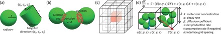
Biocellion API illustrations. (a) Biocellion, by default, maps a cell to a sphere (left). Users can add additional state variables to map an agent to a different shape—e.g. cylinder (right). Cell shape affects cell–cell shoving and adhesion, and providing mathematics to model mechanical interactions between agents is users’ task. (b) A junction between a discrete agent pair. A junction end holds a set of variables to represent the junction state in each discrete agent’s boundary. (c) A single grid box (black) and its 26 neighboring boxes (white). Each grid box covers a subregion of the simulation domain. (d) PDE parameters are set for each interface grid box based on the states of the grid box, and the discrete agents in the box. β are set for the face between two adjacent grid boxes

2.3.2 Evaluating direct interactions

This module evaluates interactions between discrete agent pairs via direct contact. Direct interactions include cell–cell shoving and adhesion, immune cells engulfing pathogens (phagocytosis), blood vessel tip cells connecting to an existing blood vessel segment (anastomosis), horizontal gene transfer by bacterial conjugation or any other interactions via direct contact between discrete agents. Biocellion users set the maximum direct interaction distance for each discrete agent type. For direct interactions between two discrete agents with different types, Biocellion sets the maximum direct interaction distance by averaging the maximum direct interaction distances of the two types. Biocellion’s role is to enumerate every agent pair within the maximum direct interaction distances, and model routines evaluate direct interactions between an agent pair.

Cell–cell interactions often depend on previous interactions. For example, if two cells form an adherens junction, pulling the two cells apart requires greater force. Biocellion supports users to explicitly form and break a junction between two discrete agent pairs (Fig. 1b). Two discrete agents forming a junction have a set of variables associated with the junction end in each cell’s boundary. Users set the number of variables for each junction end type. For example, a modeler can add a variable to store the molecular concentration of adhesion molecules if the model requires the variable to evaluate the strength of cell adhesion. A junction automatically breaks if the distance between the discrete agent pair forming the junction exceeds the maximum direct interaction distance.

Direct interactions are evaluated in parallel. If a discrete agent directly interacts with more than one agent, discrete agent variables representing the changes due to direct interactions can be updated by multiple user routine calls. This requires a coordination method if a single variable is concurrently updated by multiple user routine calls. Biocellion supports two different mechanisms to resolve conflicts—users select the conflict resolution scheme. The overwrite scheme reflects only one of the multiple updates from multiple user routine invocations. The delta scheme sums the differences from the initial value. Changes are reflected only after interactions between every pair within the interaction ranges are evaluated. Say a modeler wishes to evaluate the mechanical stress on a cell by summing the overlap distances between the cell and its neighboring cells. The delta scheme is appropriate to sum the overlap distances. If multiple immune cells are trying to engulf a pathogen agent, a modeler may expect only one immune cell to succeed. Assume the modeler added a state variable to the pathogen agent type to store the identifier of an engulfing cell. If multiple model routine calls attempt to update the variable, only one attempt will succeed with the overwrite scheme. In the next time step, the model routine compares the variable value and the interacting immune cell’s identifier, and if the two values coincide, the routine updates relevant state variables to complete phagocytosis (e.g. add the pathogen agent’s mass to the mass of the engulfing cell). This requires two time steps. We propose to add the third transactional scheme to simulate phagocytosis in a single time step in a more natural way. Two model routine calls will be serialized if they update variables associated with the same discrete agent, and the changes will be reflected immediately.

2.3.3 Updating the extracellular environment

The environment update module modifies variables representing the extracellular space by either following model-specific rules or solving PDEs. The extracellular space is partitioned into a set of cubical grid boxes. Biocellion invokes a model routine updating state variables associated with grid boxes based on model-specific rules for each grid box. In a single invocation, the model routine can read and update variables associated with one grid box and its 26 neighboring grid boxes (Fig. 1c). Variables associated with a single grid box can be updated by up to 27 model routine invocations, and Biocellion supports conflict resolution schemes similar to the above case, evaluating direct interactions between discrete agents.

Biocellion provides PDE solvers for steady-state linear reaction-diffusion PDE, time-dependent linear reaction-diffusion PDE and time-dependent reaction-diffusion PDE adopting the splitting scheme (Strang, 1968). The third method is added to model non-linear reactions among different molecular species in the extracellular space—e.g. enzymatic hydrolysis breaks macro molecules into smaller molecules suitable for cell consumption.

2.4 Simulation domain

Biocellion partitions the simulation domain into a set of cubical grid boxes. This interface grid is imposed on the simulation domain to model the environment. Different simulation modules interface through this grid (Fig. 1d).

The interface grid spacing becomes the finest grid spacing in AMR. Users set the number of AMR levels, the refinement ratio between two consecutive AMR levels, and tag each grid box with a desired AMR level. Biocellion generates an AMR grid hierarchy based on this information.

Biocellion allows users to set subregions of the simulation domain as PDE buffers—these regions are relevant only in solving PDEs. To model yeast cells growing on top of a thick agarose cylinder, modelers need to include the agarose cylinder to track molecular concentration changes by solving PDEs. However, maintaining data structures to simulate all three computational modules at the granularity of the interface grid spacing is a significant waste in both computing and memory if no cells reside in the agarose cylinder. If a subregion of the simulation domain is marked as a PDE buffer, Biocellion maintains only data structures necessary to solve PDEs. Biocellion also automatically tags the PDE buffer regions with the coarsest AMR level.

The environmental structure often limits cell movement—e.g. bacterial cells can be assumed to reside only in pore regions in soil structure (Resat et al., 2011). Updating cell displacements considering the soil structure can be a cumbersome programming task. Biocellion users can mark subregions of the simulation domain as uninhabitable, and Biocellion automatically adjusts cell displacements (set by users) to prevent cells from penetrating into an uninhabitable region.

2.5 Time steps

Biocellion asks users to set multiple time step sizes representing multiple timescales. The baseline time step is the largest time step to simulate direct interactions between discrete agents and discrete agent movement, division, death and secretion. The direct interaction module reflects the changes from the other two modules in every baseline time step. Biocellion users can tightly couple the discrete agent state update module and the environment update module by splitting a single baseline time step into multiple state-and-grid time steps. A single state-and-grid time step can be further partitioned into multiple PDE time steps. Figure 2 summarizes the integration strategy for coupling multiple simulation components.

Fig. 2.

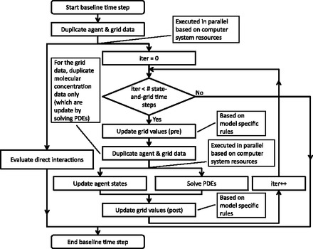
The integration strategy for coupling simulation components. Duplicating data allows parallel execution of simulation components based on system resources. For example, direct interactions are evaluated using the agent state and grid data duplicated at the beginning of the baseline time step. (note that agent and grid data are concurrently updated by other simulation components)

2.6 API highlights

Biocellion users provide model specifics in a predefined set of functions spread in five files. model_routine_config.cpp initializes the model—e.g. sets the interface grid spacing. model_routine_agent.cpp updates the discrete agent state. model_routine_grid.cpp updates the extracellular environment. model_routine_mech.cpp evaluates direct interactions between discrete agents. model_routine_output.cpp updates simulation output data—we use Paraview (http://paraview.org) for visualization.

Code 1 presents the syntax of the model routine updating the discrete agent state. Code 2 depicts the syntax of the model routine updating the net molecule production rate (PDE parameter) for a grid box. Users fill the function body to provide model specifics.

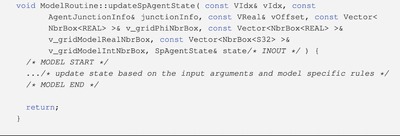
Code 1 Model routine template to update the state of a discrete agent. vIdx points to the interface grid box this discrete agent resides in. junctionInfo stores the junctions between this discrete agent and neighboring discrete agents. vOffset is the offset within the interface grid box. v_gridPhiNbrBox, v_gridModelRealNbrBox and v_gridModelIntNbrBox provide the molecular concentrations and other model-specific attribute values for this interface grid box and the 26 neighboring boxes. This model routine updates state, which holds the state variables of this discrete agent. Users fill the function body (surrounded by/* MODEL START */and/* MODEL END */) to provide model specific rules to update agent state variables.

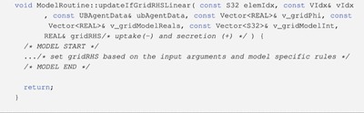
Code 2 Model routine template to set the net molecule production rate (s in Fig. 1d) for an interface grid box based on the state of the box and the states of the discrete agents residing in the box.

3 RESULTS

We implement three different models using Biocellion as case studies. The following presents cell sorting (Graner and Glazier, 1992), microbial patterning in communities of different yeast strains engaging in metabolic interactions (Momeni et al., 2013) and a bacterial system in complex soil structures (Resat et al., 2011). Full source code for the presented model implementations is included in the Biocellion release, and steps to port the microbial patterning model to Biocellion are described in (Kang et al., 2014).

3.1 Cell sorting

Many multicellular patterns formed during morphogenesis and embryonic development arise because of differential adhesion among distinct types of disassociated cells (Steinberg, 1963). Simulations of this process have demonstrated how changes in homotypic and heterotypic adhesion can result in many distinct macroscopic cellular arrangements including clumping, where homotypic cells aggregate, or mosaics, where heterotypic cells alternate forming checkerboard-like patterns (Graner and Glazier, 1992). In our model, two different cell types are defined with each cell mapped to a sphere of 8 μm diameter. If there is an overlap between two neighboring spheres, the two cells push each other to remove the overlap. If two non-overlapping cells of a same type are within 10 μm, they pull toward each other, modeling stronger adhesion. If they are of different types, there is no adhesion. The simulations demonstrate that such differential adhesion leads to cell sorting into homotypic aggregations from an initial random distribution (Fig. 3a).

Fig. 3.

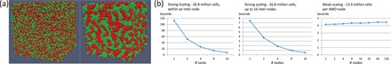
Cell sorting on Biocellion. (a) Biocellion simulation output for cell sorting. Different types of cells have different colors (red and green). (b) We present strong scaling results (solving a fixed size problem using a larger computer) and weak scaling results (solving a larger problem using a larger computer increasing the problem size proportional to the computer size). For the strong scaling results (left and center), we used up to 16 Intel nodes (each node has two Intel Xeon E-5 2670 2.6 GHz sockets). For the weak scaling results (right), we used up to 128 AMD nodes (each node has two AMD Opteron 6272 Interlago 2.1 GHz sockets) in a larger cluster. We measured the execution time per step (evaluating pairwise interactions between every cell pair within 10 μm, cell packing density: 1.6 cells/${(10\text{μm})}^3$). Biocellion reduces the execution time by 15.1 times using 16 cores in an Intel node (left) and by additional 15.8 times using 16 Intel nodes. This reduces the execution time per step to sort 26.8 million cells from 113 to 0.474 s. Biocellion sorts a larger system of cells with little increase in time, so long as we increase the number of nodes proportional to the cell system size. Biocellion sorts 1.72 billion cells in 4.46 s per step using 128 AMD nodes (right). No model code change is necessary to achieve this speedup

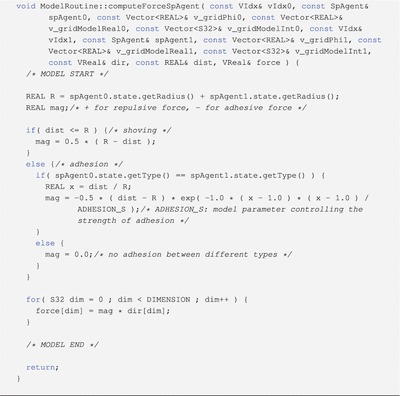
Code 3 The model routine simulating shoving and differential adhesion between two cells. A modeler focuses on describing mathematical rules to evaluate shoving and differential adhesion. Concurrently executing this model routine using parallel computers for different sets of agent pairs is Biocellion’s responsibility.

The model code implemented using Biocellion has 854 lines—the empty template has 723 lines. Code 3 shows the model routine evaluating cell–cell shoving and differential adhesion. Biocellion users can simulate cell sorting using a cluster computer with little more than 100 lines of coding—the Biocellion framework code has nearly 100 thousand lines to simulate the model using efficient algorithms (briefed in Section 2.2) and parallel computers.

Figure 3b summarizes the performance results. Our results sort up to 1.72 billion cells. In comparison, Chen et al. (2007) adopted the Cellular Potts model and sorted 4 million cells placed on a 2D 10 000² lattice using 25 compute nodes (each node has two AMD Opteron 248 sockets) taking 5.3 s per Monte Carlo step. Tapia and D’Souza also adopted the Cellular Potts model and sorted 1.46 million cells placed on a 3D 256³ lattice using a NVIDIA Tesla C1060 GPU taking 0.26 s per Monte Carlo step (Tapia and D’Souza, 2011). Jeannin-Girardon et al. (2013) adopted an agent-based model mapping a cell to seven particles and sorted 1 million cells using a NVIDIA GTX 690 GPU taking little longer than 0.4 s per step. Even though we are comparing results from running different models on a variety of different computers, and perform varying amounts of work per step, our work significantly advances the state of the art by scaling to the largest parallel computers and sorting billions of cells, three orders of magnitude more than prior work.

3.2 Microbial patterning

Momeni et al. (2013) have studied pattern formation in communities of yeast strains based on their ecological interaction types, comparing the MATLAB simulation output and actual patterns observed in laboratory experiments. We implemented one test case in their work using Biocellion (Fig. 4 visualizes the simulation output). One strain (say the R strain) produces adenine and consumes lysine. Another strain (say the G strain) produces lysine and consumes adenine. The two strains grow on top of a 24 mm thick agarose cylinder—the height of the simulated colony growth region in the original paper is 300 μm in comparison. Momeni et al. demonstrated that the cooperative relationship between the two strains promotes the intermixing of the two yeast strains.

Fig. 4.

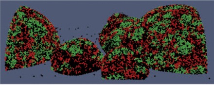
Microbial patterns produced using Biocellion. The cooperative relationship between R (black) and G (green) strain cells promote the intermixing of the two strains. Black spheres are dead cells

Momeni et al.’s original implementation sets the PDE grid spacing to 50 μm for the entire simulation domain (to track adenine and lysine concentrations, the maximum cell diameter is 5 μm in comparison). Adenine concentration has high spatial variation near adenine-producing cells. A grid of 50 μm spacing might be sufficient to model intermixing patterns (especially when diffusion is fast), but 5 μm grid spacing is required to capture the high spatial variation—this might be necessary to investigate more complex problems with high fidelity. Momeni et al.’s original implementation adopts the explicit Euler method—reducing grid spacing by a factor of 10 requires reducing the time step size by 10² times for stability. The original implementation takes about a week to simulate yeast growth for 500 h with 50 μm grid spacing. Simulating with 5 μm grid spacing will take 10⁵ weeks (∼1917 years) using the original implementation—10³ times more grid boxes and 10² times more time steps. Using Biocellion, a simulation with 5 μm grid spacing finishes in little more than a week using 8 Intel nodes owing to AMR (using 5 μm grid spacing only for the yeast colony growth region and the top 40 μm of the agarose cylinder where adenine concentration is highly localized), L-stable semi-implicit method for time-stepping, and parallel computing (exploiting multiple cores in a node and up to eight nodes, Biocellion reduces the execution time per baseline time step by 64.9 times).

The original MATLAB code has 449 lines (the Matlab code is available at the publisher’s site) while the Biocellion model code has 1817 lines—again, the empty template has 723 lines. The increase in the model code size is due to the increase in the model fidelity. The original MATLAB implementation partitions the simulation domain into fixed size cubical boxes and maps a cell to a box. On cell division, the daughter cell occupies one of the nearest boxes, instantly pushing surrounding cells outward. This models neither cell size changes nor cell movement due to cell–cell shoving (cells move only because of cell division). Cells divide always vertically when surrounded by other cells, and this simplification ends up underestimating the degree of intermixing in the vertical direction (Momeni et al., 2013). The Biocellion model code maps cells to spheres and more faithfully models cell growth (by increasing the radius of a cell) and cell–cell shoving (by removing the overlap between two spheres). Cells divide in a random direction instead of always dividing vertically. The model improvements result in more accurate reproduction of the intermixing patterns seen in laboratory experiments (Kang et al., 2014). The Matlab code includes many large matrix operations. This reduces the code size and improves the performance using Matlab’s optimized matrix operation libraries but does not provide sufficient flexibility to implement complex cell behavioral rules.

3.3 Bacterial system in soil aggregate

Resat et al. (2011) have investigated enzymatic macro-molecule (cellulose) hydrolysis by a heterogeneous population of bacteria in complex soil structure. A soil structure has blocked regions and pore regions. No cells reside in the blocked regions and molecules cannot diffuse into the blocked regions—modelers can easily introduce these constraints into Biocellion by marking the blocked regions as uninhabitable and setting diffusion coefficients of the blocked grid box faces to 0. They consider three bacterial strains. One strain secretes a hydrolysis enzyme. The second strain expresses a hydrolysis enzyme on the cell surface. The third strain neither secretes nor expresses a hydrolysis enzyme and does not contribute to macro-molecule hydrolysis. Macro-molecules are located in blocked regions, and the original model updates the concentrations of macro-molecules and secreted enzymes bound to macro-molecules (which cannot diffuse) based on model-specific rules (instead of solving PDEs) considering the concentrations of the secreted enzyme and the cell membrane-bound enzyme in the pore boxes adjacent to the blocked boxes containing macro-molecules. The original model updates secreted enzyme and glucose (output of the enzymatic hydrolysis) concentrations by solving PDEs. Biocellion users can update state variables associated with grid boxes based on model-specific rules (in addition to solving PDEs) to serve this modeling requirement.

The original model studied the efficiency of enzymatic hydrolysis and cell growth dynamics for micro-pores and small porous soil aggregates. A single simulation of a 111 μm × 111 μm × 111 μm soil aggregate takes 2–4 days on a workstation using the original Fortran implementation (8457 lines). Using Biocellion (the model code has 2466 lines), simulating a soil structure composed of multiple aggregates (384 μm × 384 μm × 384 μm) takes a comparable amount of time using four Intel nodes (exploiting multiple cores in a node and up to four nodes, Biocellion reduces the execution time per baseline time step by 47.5 times). Biocellion users can increase the simulation size using a bigger computer without additional programming if it is necessary to study more complex and larger scale phenomena.

4 DISCUSSION AND FUTURE WORK

The Biocellion API does not assume a specific parallel computer architecture. Biocellion users can test their initial implementations on a desktop PC first and scale-up their simulations on Cloud computers or supercomputers with no code change—the complexity of the model code depends only on the complexity of the mathematical model and is irrelevant to the underlying computer system.

Biocellion already simulates millions to billions of cells in the 3D environment using multicore workstations to moderate sized cluster computers. Model code conforming to the Biocellion API will seamlessly benefit from Biocellion updates on improving scalability and performance—e.g. tuning for accelerator architectures such as Intel Xeon Phi. We maintain that the computational complexity of high fidelity models and the difficulty of parallel programming for current and future computers should not be a major bottleneck in building highly practical biological system models.

4.1 Limitations and future work

Representing a cell by multiple agents allows modeling cell shapes and physical interactions in greater detail (Jeannin-Girardon et al., 2013; Newman, 2005). Mapping a cell to multiple agents is also necessary to separately model subcellular compartments and to represent the spatial variation of molecular concentrations within a cell. However, Biocellion does not yet support this. This limits the maximum resolution used to represent the environment because the interface grid spacing cannot be less than the maximum direct interaction distance between two agents—which often coincides with the maximum cell diameter if a cell is mapped to an agent. Mapping a cell to multiple smaller agents will allow modeling the environment at higher resolution. We plan to extend Biocellion to support multi-agent representation of a cell to lift these limitations.

Biocellion provides deterministic ODE system solvers, but there are many other approaches (Shmulevich and Aitchison, 2009) or even a combination of various approaches (Karr et al., 2012) to model cell regulatory networks. Users need to implement solvers on their own to use those approaches. This increases the programming burden and lowers the performance, as modelers are likely to write less efficient code than HPC experts. We plan to add solvers for widely used modeling approaches to further reduce the programming burden in simulating cell regulatory networks.

Biocellion asks users to represent a model using a predefined set of model routines describing how a cell behaves, how a cell directly interacts with neighboring cells and how cells in a small region interact with their microenvironment. The Biocellion model routines provide local behavioral rules. Global processes, such as water or blood flow, cannot be modeled using the local rules unless Biocellion provides solvers to simulate global processes using locally determined parameter values. We plan to add solvers for Navier-Stokes equations (to compute flow rates) and advection-reaction-diffusion equations (to update molecular concentrations considering flow) to support water and blood flow modeling.

Flexibility, performance, and usability often conflict in software design. We designed Biocellion to allow a modeler with strong mathematical modeling background (but without HPC expertise) to build high fidelity models—we focus on providing high flexibility to support various modeling requirements even though we do not ignore usability. To reach a broader range of users, we envision adding productivity layers on top of Biocellion once mathematical modeling of biological systems matures. Biocellion will serve as an acceleration layer for higher productivity tools in such cases.

REFERENCES

- Anderson ARA, Chaplain MAJ. Continuous and discrete mathematical models of tumor-induced angiogenesis. Bull. Math. Biol. 1998;60:857–899. doi: 10.1006/bulm.1998.0042. [DOI] [PubMed] [Google Scholar]
- Andrews SS. Spatial and stochastic cellular modeling with the smoldyn simulator. Methods Mol. Biol. 2012;804:519–542. doi: 10.1007/978-1-61779-361-5_26. [DOI] [PubMed] [Google Scholar]
- Bernholdt DE. Proceedings Symposium on Component and Framework technology in high-performance and scientific computing (CompFrame) Montreal, Canada: 2007. Component architectures in the next generation of ultrascale scientific computing: challenges and opportunities. [Google Scholar]
- Borgdorff J, et al. Distributed multiscale computing with MUSCLE 2, the multiscale coupling library and environment. J. Comput. Sci. 2014;5:719–731. [Google Scholar]
- Briggs WL, et al. A Multigrid Tutorial. Philadelphia, PA, USA: SIAM; 2000. [Google Scholar]
- Byrne H, Drasdo D. Individual-based and continuum models of growing cell populations: a comparison. J. Math. Biol. 2009;58:657–687. doi: 10.1007/s00285-008-0212-0. [DOI] [PubMed] [Google Scholar]
- Chen N, et al. A parallel implementation of the cellular potts model for simulation of cell-based morphogenesis. Comput. Phys. Commun. 2007;176:670–681. doi: 10.1016/j.cpc.2007.03.007. [DOI] [PMC free article] [PubMed] [Google Scholar]
- Chin LS, et al. Technical report. STFC Rutherford Appleton Laboratory; 2012. Flame-ii: a redesign of the flexible large-scale agent-based modelling environment. [Google Scholar]
- Colella P, et al. Chombo Software Package for AMR Applications Design Document. Berkeley, CA, USA: Lawrence Berkeley National Laboratory; 2012. [Google Scholar]
- Daly MJ. Engineering radiation-resistant bacteria for environmental biotechnology. Curr. Opin.Biotechnol. 2000;11:280–285. doi: 10.1016/s0958-1669(00)00096-3. [DOI] [PubMed] [Google Scholar]
- Ferrer J, et al. Individual-based modelling: an essential tool for microbiology. J. Biol. Phys. 2008;34:19–37. doi: 10.1007/s10867-008-9082-3. [DOI] [PMC free article] [PubMed] [Google Scholar]
- Frieboes HB, et al. Three-dimensional multispecies nonlinear tumor growthII: tumor invasion and angiogenesis. J. Theor. Biol. 2010;264:1254–1278. doi: 10.1016/j.jtbi.2010.02.036. [DOI] [PMC free article] [PubMed] [Google Scholar]
- Graner F, Glazier J. Simulation of biological cell sorting using a two-dimensional extended Potts model. Phys. Rev. Lett. 1992;69:2013–2016. doi: 10.1103/PhysRevLett.69.2013. [DOI] [PubMed] [Google Scholar]
- Iserles A. Numerical Analysis of Differential Equations. Cambridge, UK: Cambridge University Press; 2009. [Google Scholar]
- Izaguirre JA, et al. COMPUCELL, a multi-model framework for simulation of morphogenesis. Bioinformatics. 2004;20:1129–1137. doi: 10.1093/bioinformatics/bth050. [DOI] [PubMed] [Google Scholar]
- Jeannin-Girardon A, et al. An efficient biomechanical cell model to simulate large multi-cellular tissue morphogenesis: application to cell sorting simulation on GPU. Lect. Notes Comput. Sci. 2013;8273:96–107. [Google Scholar]
- Jiao Y, Torquato S. Emergent behaviors from a cellular automaton model for invasive tumor growth in heterogeneous microenvironments. PLoS Comput. Biol. 2011;7:e1002314. doi: 10.1371/journal.pcbi.1002314. [DOI] [PMC free article] [PubMed] [Google Scholar]
- Kang S, Kahan S. Biocellion 1.1 User Manual. Richland, WA, USA: Pacific Northwest National Laboratory; 2014. [Google Scholar]
- Kang S, et al. Algorithm engineering challenges in multicore and manycore systems. Inf. Technol. 2011;53:266–273. [Google Scholar]
- Kang S, et al. Simulating microbial community patterning using biocellion. Methods Mol. Biol. 2014;1151:233–253. doi: 10.1007/978-1-4939-0554-6_16. [DOI] [PubMed] [Google Scholar]
- Karr JR, et al. A whole-cell computational model predicts phenotype from genotype. Cell. 2012;150:389–401. doi: 10.1016/j.cell.2012.05.044. [DOI] [PMC free article] [PubMed] [Google Scholar]
- Lardon LA, et al. iDynoMiCS: next-generation individual-based modelling of biofilms. Environ. Microbiol. 2011;13:2416–2434. doi: 10.1111/j.1462-2920.2011.02414.x. [DOI] [PubMed] [Google Scholar]
- Loew LM, Schaff JC. The virtual cell: a software environment for computational cell biology. TRENDS Biotechnol. 2001;19:401–406. doi: 10.1016/S0167-7799(01)01740-1. [DOI] [PubMed] [Google Scholar]
- McDougall SR, et al. Mathematical modelling of flow through vascular networks: implications for tumour-induced angiogenesis and chemotherapy strategies. Bull. Math. Biol. 2002;64:673–702. doi: 10.1006/bulm.2002.0293. [DOI] [PubMed] [Google Scholar]
- Meagher D. Geometric modeling using octree encoding. Comput. Graph. Image Process. 1982;19:129–147. [Google Scholar]
- Melnicki MR, et al. Feedback-controlled LED photobioreactor for photophysiological studies of cyanobacteria. Bioresour. Technol. 2013;134:127–133. doi: 10.1016/j.biortech.2013.01.079. [DOI] [PubMed] [Google Scholar]
- Minar N, et al. Technical report. Santa Fe Institute; 1996. The SWARM simulation system: a toolkit for building multi-agent simulations. [Google Scholar]
- Momeni B, et al. Strong inter-population cooperation leads to partner intermixing in microbial communities. eLife. 2013;2:e00230. doi: 10.7554/eLife.00230. [DOI] [PMC free article] [PubMed] [Google Scholar]
- Newman TJ. Modeling multicellular systems using subcellular elements. Math. Biosci. Eng. 2005;2:611–622. doi: 10.3934/mbe.2005.2.613. [DOI] [PubMed] [Google Scholar]
- Resat H, et al. Modeling microbial dynamics in heterogeneous environments: growth on soil carbon sources. Microb. Ecol. 2011;63:883–897. doi: 10.1007/s00248-011-9965-x. [DOI] [PubMed] [Google Scholar]
- Shmulevich I, Aitchison JD. Deterministic and stochastic models of genetic regulatory networks. Methods Enzymol. 2009;467:335–356. doi: 10.1016/S0076-6879(09)67013-0. [DOI] [PMC free article] [PubMed] [Google Scholar]
- Starruß J, et al. Morpheus: a user-friendly modeling environment for multiscale and multicellular systems biology. Bioinformatics. 2014;30:1331–1332. doi: 10.1093/bioinformatics/btt772. [DOI] [PMC free article] [PubMed] [Google Scholar]
- Steinberg MS. Reconstruction of tissues by dissociated cells. Some morphogenetic tissue movements and the sorting out of embryonic cells may have a common explanation. Science. 1963;141:401–408. doi: 10.1126/science.141.3579.401. [DOI] [PubMed] [Google Scholar]
- Strang G. On the construction and comparison of difference schemes. SIAM J. Numer. Anal. 1968;5:506–517. [Google Scholar]
- Tapia JJ, D’Souza RM. Parallelizing the cellular potts model on graphics processing units. Comput. Phys.Commun. 2011;182:857–865. [Google Scholar]
- Voss-Böhme A. Multi-scale modeling in morphogenesis: a critical analysis of the cellular potts model. PLoS One. 2012;7:1–14. doi: 10.1371/journal.pone.0042852. [DOI] [PMC free article] [PubMed] [Google Scholar]
- Weinberg RA. The Biology of Cancer. New York, NY, USA: Garland Science; 2007. [Google Scholar]
- Xavier JB, et al. Social evolution of spatial patterns in bacterial biofilms: when conflict drives disorder. Am. Nat. 2009;174:1–12. doi: 10.1086/599297. [DOI] [PubMed] [Google Scholar]