Optical coherency matrix tomography

Abstract

The coherence of an optical beam having multiple degrees of freedom (DoFs) is described by a coherency matrix G spanning these DoFs. This optical coherency matrix has not been measured in its entirety to date—even in the simplest case of two binary DoFs where G is a 4 × 4 matrix. We establish a methodical yet versatile approach—optical coherency matrix tomography—for reconstructing G that exploits the analogy between this problem in classical optics and that of tomographically reconstructing the density matrix associated with multipartite quantum states in quantum information science. Here G is reconstructed from a minimal set of linearly independent measurements, each a cascade of projective measurements for each DoF. We report the first experimental measurements of the 4 × 4 coherency matrix G associated with an electromagnetic beam in which polarization and a spatial DoF are relevant, ranging from the traditional two-point Young’s double slit to spatial parity and orbital angular momentum modes.

The statistical fluctuations of light in space and time may be characterized by a hierarchy of correlation functions for electromagnetic field components¹,². These functions, not the optical fields themselves, provide a description of light in terms of observable quantities³. The theory of optical coherence investigates the properties of these correlation functions pertaining to the temporal, spatial, and polarization degrees of freedom (DoFs). When these DoFs are uncoupled (or uncorrelated), simple measures of coherence for each DoF suffice, such as coherence time, coherence area, and degree of polarization⁴. However, when the DoFs are coupled, such measures lose their utility and more sophisticated approaches are required, such as the mutual coherence function⁵, the beam coherence-polarization matrix⁶,⁷,⁸, or the 4 × 4 field correlation matrix for a pair of points in an electromagnetic field⁹,¹⁰,¹¹.

While the importance of coupling between DoFs was recognized decades ago, as in Mandel’s seminal work on optical cross-spectral purity (the absence of spatial-spectral coupling)¹², recent advances have led to a host of scenarios wherein such coupling is critical. For example, vector beams correlate polarization with spatial position¹³, scattering from complex photonic structures and devices may couple the relevant field DoFs¹⁴,¹⁵, and reliance on multimode optical fibers for spatial multiplexing is reviving interest in joint polarization-spatial-mode characterization¹⁶. In exploring these settings, it has recently proven fruitful to adopt the Hilbert-space formulation used in quantum mechanics to the needs of classical coherence theory¹⁰,¹¹—an approach that has early prescient antecedents¹⁷,¹⁸. In the context of coupling between multiple DoFs, such a treatment necessitates introducing the notion of ‘classical entanglement’¹⁰,¹⁹,²⁰,²¹,²²,²³,²⁴,²⁵. In quantum mechanics, states associated with bipartite systems that do not separate into products of states belonging to the Hilbert space of each particle are said to be entangled²⁶. As a consequence of the mathematical similarity between the Hilbert spaces of multi-partite quantum states and multi-DoF classical optical fields, a corresponding concept of classical entanglement indicates the non-separability of the beam into uncoupled DoFs. After the initial suggestion by Spreeuw¹⁹, a substantial body of work has accumulated in the past five years in which classical entanglement is exploited in solving long-standing problems in polarization optics²⁷,²⁸,²⁹, delineating the contributions of non-separability and intrinsic randomness to the coherence of an optical beam¹⁰,³⁰, introducing new metrology schemes³¹, and implementing classical analogs of quantum information processing protocols, such as teleportation³²,³³, and super-dense coding, etc.

A fundamental capability that has remained elusive in classical optics is the complete identification of the coherence function for a beam with coupled DoFs. In quantum mechanics, the task of measuring all the elements of a density matrix is known as ‘quantum state tomography’³⁴,³⁵. The corresponding procedure for multi-DoF beams in classical optics has been studied theoretically¹¹, but has not been demonstrated experimentally heretofore. Even in the simplest case of two binary DoFs⁶ (e.g., polarization, a bimodal waveguide³⁶,³⁷, two coupled single-mode waveguides³⁸,³⁹, spatial-parity modes⁴⁰,⁴¹,⁴²,⁴³,⁴⁴, etc.), the associated 4 × 4 coherency matrix G, which is a complete representation of second-order coherence¹⁰,¹¹, has not been measured in its entirety to date.

Results

In this Article, we present a methodical approach—optical coherency matrix tomography (OCmT)—for measuring the complex elements of 4 × 4 coherency matrices G by appropriating the quantum-state-tomography strategy. To demonstrate the universality of our approach, we implement it with coherent and partially coherent fields having coupled or uncoupled DoFs in three distinct settings involving pairs of points⁹,¹⁰,¹¹, spatial-parity modes⁴⁰,⁴¹,⁴²,⁴³,⁴⁴, and orbital angular momentum (OAM) modes⁴⁵—each together with polarization. We identify the minimal set of linearly independent, joint spatial-polarization projective measurements that enable a unique reconstruction of G. Since G is a complete representation of the field, its reconstruction obviates the need to measure directly any coherence descriptors (all of which are scalar functions of the complex elements of G) and, moreover, allows for unambiguous identification of classical entanglement.

The coherence of an optical beam having a single binary DoF is represented by a 2 × 2 Hermitian coherency matrix , where , , and E_j is the field corresponding to one level of the DoF. For example, polarization is represented by the coherency matrix⁴

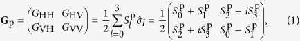where , is the horizontal (H) or vertical (V) field component at a point , are the Stokes parameters, and are the Pauli matrices

Polarization coherence is quantified by the degree of polarization —with and corresponding to purely polarized and completely unpolarized light, respectively. The Stokes parameters are evaluated via four projective polarization measurements [Fig. 1(a)]: , , and correspond to the H, diagonal (D), and right-hand-circular (R) polarization components, respectively, in addition to the total power ref. ⁴⁶; in which case . The same formalism may be applied to other binary DoFs [Fig. 1(b)]: (i) the scalar field at two points and , E_a and E_b; (ii) the spatial-parity even ‘e’ and odd ‘o’ modes of a scalar field E_e and E_o refs. ^{40, 41, 42, 43, 44}; or (iii) a pair of OAM modes, e.g., E₀ and E₁ corresponding to OAM and 1, respectively⁴⁵,⁴⁷.

Figure 1. Measurement scheme for optical coherency matrix tomography (OCmT).

(a) Four projections , to obtain the Stokes parameters {S_l} and reconstruct G_p for the polarization DoF. (b) Similarly, four projections , to obtain the Stokes parameters {S_m} and reconstruct G_s for a binary spatial DoF. (c) OCmT enables the reconstruction of G for the two binary DoFs in (a,b) considered simultaneously via 16 joint polarization-spatial measurements, each of which consists of a cascade of two projections—one from (a) and the other from (b).

When two binary DoFs of the field are relevant, e.g., the first is polarization ‘p’ and the second is a spatial ‘s’ DoF with modes identified as ‘a’ and ‘b’ [Fig. 1(c)]—the corresponding coherency matrix G is now 4 × 4 refs. ^{10, 11},

where , , E_jk is a field component with j = H, V and k = a, b, {S_lm} are the two-DoF Stokes parameters, and and are the Pauli matrices on the polarization- and spatial-DoF Hilbert subspaces, respectively¹¹. In determining the coherence descriptors of each DoF independently of the other, one first traces over the other DoF to obtain a reduced coherency matrix¹⁰. The reduced polarization coherency matrix G_p, obtained by tracing over the spatial DoF in G, is given by

while the reduced coherency matrix for the spatial DoF G_s, obtained after tracing over polarization in G (see ref. 11), is given by

The elements of the reduced coherency matrices are measured by a system sensitive to one DoF, but not to the other. When the two DoFs are uncoupled, then , otherwise the elements of G_p and G_s lack information about the correlations between the two DoFs that is contained in G. Such correlations are only measurable by a system that is sensitive to both DoFs via joint polarization-spatial measurements.

We pose the following question: what are the necessary and sufficient measurements to reconstruct an arbitrary G for two binary DoFs? This question was solved by Wootters⁴⁸ in the context of reconstructing the density matrix for a bipartite quantum system. He showed that the measurements carried out on each subsystem to reconstruct its reduced density matrix are sufficient to reconstruct when carried out jointly—a methodology known as quantum state tomography³⁴,³⁵. In our context of a classical optical beam having two binary DoFs, the analogy with the quantum setting allows us to exploit the same strategy. Regardless of the specific form of G, the necessary measurements to carry out OCmT and reconstruct G [Fig. 1(c)] are those used to reconstruct the reduced coherency matrices [Fig. 1(a,b)] carried out in cascades of pairs of projections—one for polarization and the other for the spatial DoF. Each measurement yields a real number I_lm (projection l for polarization and m for the spatial DoF) corresponding to the projection of a tomographic slice through G. The 16 combinations of polarization-spatial measurements are inverted to obtain the two-DoF Stokes parameters, , and hence reconstruct G (see ref. 11 for details).

We have performed a series of experiments implementing the OCmT scheme described above using quasi-monochromatic beams having two binary DoFs: polarization and a spatial DoF. We have measured the 4 × 4 coherency matrix G for six different beams corresponding to distinct states of light having the following properties:

G₁: the polarization and spatial DoFs are separable and both are coherent.

G₂: the polarization DoF is coherent while the spatial DoF lacks coherence.

G₃: both the polarization and spatial DoFs lack coherence.

G₄: the polarization and spatial DoFs are classically entangled.

G₅: the polarization and spatial DoFs are classically correlated.

G₆: this beam is a mixture of the separable-coherent beam G₁ and the classically entangled beam G₄.

We use the sequence of polarization projections described earlier and present below the spatial projections following the H projection (similar spatial projections are carried out following the V, D and R polarization projections).

Polarization with Spatial Position

The first realization of the spatial DoF is the traditional two points, as in the Young’s double slit experiment. The polarization and position-coupled beam is prepared in one of six states G₁ through G₆; Fig. 2(a) (see Supplementary information for details). OCmT for a such a beam comprises of the polarization analysis followed by the spatial analysis; Fig. 2(b). The spatial analysis may alternatively be carried out by extracting specific intensity points from the far-field intensity patterns for only two values of displacement x on a screen or an array of detectors; Fig. 2(c). The four spatial projections are obtained by measuring the following: (1) the total power from both points I₁₀ = I_H at x = 0; (2) the power from point ‘a’ I₁₁ = I_Ha at x = 0; (3) the power in the far-field interference pattern at x = 0; and (4) the power at the value of x corresponding to a phase shift ; see Fig. 2(d). It is important to note that the visibility of fringes is not the parameter sought here to characterize the spatial coherence at ‘a’ and ‘b’; instead the four points identified in Fig. 2(d), together with the set of points obtained for the V, D, and R polarization projections, reveal the complete picture even when polarization and the spatial DoFs are classically entangled.

Figure 2. Polarization considered with spatial location in a Young’s double-slit configuration.

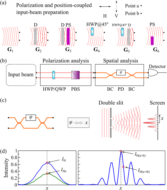
(a) Experimental setups for preparing polarization and position-coupled beams G₁ through G₆; D: diffuser that randomizes the beam spatially; PS: polarization scrambler that randomizes the beam polarization; HWP: half-wave plate. (b) Experimental setup delineating the stages of polarization analysis followed by spatial analysis. HWP: half-wave plate; QWP: quarter-wave plate; PBS: polarizing beam splitter; BC: 50:50 beam coupler; PD: phase delay element that introduces a phase shift . (c) Illustration depicting the equivalence between the phase shift introduced by the phase element PD, and the lateral displacement x on a screen upon which the far-field intensity pattern is projected. (d) Spatial profile measurements obtained by a CCD camera illustrating the spatial projective measurements for the H polarization projection; similarly for the V, D, and R projections.

Polarization with Spatial Parity

The second spatial-DoF realization makes use of one-dimensional even ‘e’ and odd ‘o’ spatial-parity modes with respect to x = 0. The polarization and spatial parity-coupled beam is prepared in one of six states G₁ through G₆; Fig. 3(a) (see Supplementary information for details). OCmT for a such a beam comprises of the polarization analysis followed by the spatial-parity analysis; Fig. 3(b). The four spatial projections are obtained by measuring the power (integrated over the shaded areas in Fig. 3(c)) in the following settings: (1) the total power I₁₀ = I_H of the beam; (2) the power of the even component I₁₁ = I_He obtained from a modified Mach-Zehnder interferometer that separates the beam into the different spatial-parity components⁴¹; (3) the power after blocking the half-plane x < 0, corresponding to a projection onto the component; and (4) a projection onto the component obtained from the power of the even component measured after first introducing a phase-step between the two plane halves x < 0 and x ≥ 0 implemented by a spatial light modulator (SLM); see Fig. 3(c). This phase modulation was shown in ref. 40, 41, 42, 43, 44 to produce a rotation on a major circle on a Poincaré sphere having the e and o modes as antipodes.

Figure 3. Polarization considered with spatial parity modes.

(a) Experimental setups for preparing polarization and spatial-parity-coupled beams G₁ through G₆; HWP: half-wave plate; SLM: spatial light modulator; PS: polarization scrambler that randomizes the beam polarization. (b) Experimental setup delineating the stages of polarization analysis followed by spatial-parity analysis. HWP: half-wave plate; QWP: quarter-wave plate; PBS: polarizing beam splitter; SLM: spatial light modulator; BS: beam splitter; SF: spatial flipper that flips the sign of the odd ‘o’ spatial-parity mode, leaving the even ‘e’ mode intact. (c) Corresponding spatial profile measurements obtained by a CCD camera illustrating the spatial projective measurements for the H polarization projection; similarly for the V, D, and R projections.

Polarization with OAM

The third realization exploits two low-order OAM modes and . The polarization and OAM-coupled beam is prepared in one of six states G₁ through G₆; Fig. 4(a) (see Supplementary information for details). OCmT for a such a beam comprises of the polarization analysis followed by the OAM mode analysis; Fig. 4(b).The four spatial projections are obtained by measuring the following: (1) the total power I₁₀ = I_H; (2) the power of the component obtained using a spatial filter (a lens focusing to a single-mode fiber); (3) the power of the component using a phase vortex with the dislocation displaced laterally with respect to the beam implemented using an SLM ref. ⁴⁹; and (4) the power of the component using the same phase vortex but with the dislocation displaced vertically ; see Fig. 4(c).

Figure 4. Polarization considered with OAM modes.

(a) Experimental setups for preparing polarization and OAM-coupled beams G₁ through G₆; HWP: half-wave plate; SLM: spatial light modulator; PS: polarization scrambler that randomizes the beam polarization. (b) Experimental setup delineating the stages of polarization analysis followed by OAM-mode analysis. HWP: half-wave plate; QWP: quarter-wave plate; PBS: polarizing beam splitter; SLM: spatial light modulator; FC: fiber coupler; SMF: single-mode fiber. (c) Corresponding spatial profile measurements obtained by a power-meter illustrating the spatial projective measurements for the H polarization projection; similarly for the V, D, and R projections. Spatial measurements are obtained by dislocating the phase singularity 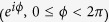relative to the beam Δx along x and Δy along y. I_H is obtained by adding the intensities at (σ is the beam width) and at Δx = 0, is obtained at , and is obtained at (Δx_mid and Δy_mid are calibrated using a Gaussian beam).

Measurements

We have measured the complex elements of G for six different classes of beams comprising those with separable DoFs (both coherent, both incoherent, or in a hybrid coherent/incoherent configuration), non-separable DoFs (classically entangled or classically correlated), and mixtures of beams from the two separable and non-separable classes (see Supplementary information for the complete results). In each experiment, the prepared beam passes first through polarization then spatial-DoF analysis stages (the order may be reversed without changing the outcome). In each of these realizations, permutations of the four polarization projection settings combined with the four spatial projection settings yield 16 measurements for OCmT, which are used to reconstruct G. We make use of a maximal-likelihood algorithm that exploits the constraints set by the trace, hermiticity, and semi-positive-definiteness of G⁵⁰. We portray the real and imaginary components of G using the standard visualization from quantum state tomography. In each plot we provide the coherence descriptor for the polarization D_p and spatial DoF D_s obtained from their reduced coherency matrices, in addition to the linear entropy , which serves as a measure of the overall beam coherence, where D_G ranges from 0 (complete incoherence in all DoFs) to 1 (a coherent beam with no statistical fluctuations)⁵¹. Finally, we provide the fidelity as a measure of the robustness of the reconstruction process via OCmT⁵², where Γ is the theoretical matrix and G is the measured matrix.

Beams with separable DoFs

We present in Fig. 5 three examples of beams having separable DoFs, . First, both polarization and spatial DoFs are coherent, [Fig. 5(a)]. Second, a hybrid beam in which polarization is pure (along D) but the beam is spatially incoherent, [Fig. 5(b)]. Third, a completely incoherent beam [Fig. 5(c)]. In all three cases, the separability of the two DoFs is readily detected by visual inspection of G and confirmed by taking the direct product of the reduced coherency matrices.

Figure 5. Measurements of G for beams having separable DoFs.

(a) G₁: both DoFs are coherent; (b) G₂: polarization is coherent but the spatial DoF is incoherent; and (c) G₃: both DoFs are incoherent. In each case, the reduced coherency matrices G_p and G_s are also depicted. The imaginary components are negligible, and are not shown.

Beams with non-separable DoFs

We next present two fundamentally distinct classes of beams with non-separable G in Fig. 6(a,b). First, OCmT of a classically entangled beam G₄ is shown in Fig. 6(a), wherein the beam is fully coherent, and yet the measures extracted from reduced coherency matrices indicate complete incoherence. In such a beam, the polarization and spatial modes occur in pairs—e.g., H with ‘a’ and V with ‘b’ (but never H with ‘b’ or V with ‘a’). In the traditional view of the double slit experiment, such coupling will produce no interference fringes, and the lack of visibility may be interpreted as the absence of spatial coherence, despite the beam being perfectly spatially coherent. This coupling between the DoFs is in fact encoded in the non-zero off-diagonal elements of G revealed once it is reconstructed through OCmT, but cannot be obtained from G_p or G_s. Second, a classically correlated beam G₅ is shown in Fig. 6(b) in which the same coupling between polarization and spatial modes occurs as in the previous example, except the different combinations are incoherently mixed and not linearly superposed. The partial global coherence—despite the complete lack of coherence for each DoF—is clear from the fact that not all the diagonal elements of G₅ are equal as is the case in G₃.

Figure 6. Measurements of G for beams having non-separable DoFs.

(a) G₄: classically entangled beam; and (b) G₅: classically correlated beam. The imaginary components in both cases are negligible, and are not shown. (c) Measurement of the real and imaginary parts of G₆: mixture of beams G₁ and G₄. In each case, the reduced coherency matrices G_p and G_s are also depicted.

Mixture of beams with separable and non-separable DoFs

Finally, in Fig. 6(c) we depict G₆ corresponding to a beam formed by statistically mixing the separable-coherent beam G₁ and the classically entangled beam G₄. The measurement of G₆ indicates that part of the apparent incoherence in this beam stems from the intrinsic randomness in the individual DoFs, and part of it from the correlation, or classical entanglement, between the two DoFs.

Discussion

The reconstruction of G allows for the unambiguous and complete mathematical expression of fields that are coherent, partially coherent, or incoherent, in either, or both, DoFs of an optical beam with two binary DoFs. The usefulness of this technique becomes specially apparent in cases where the DoFs are coupled or non-separable, and the traditional scalar measures of coherence provide a conflicting and fallacious account of beam coherence. The apparent absence of coherence in any DoF may be the result of intrinsic randomness due to statistical fluctuations, or due to the coupling or non-separability with another DoF. In the latter case, the measurement of G also provides the way for implementing unitary transformations required to undo such coupling, and restore coherence in the DoFs. The application of our work can be easily seen in the myriad applications of coherence under conditions of coupled DoFs, particularly those involving localized vector beams, sub-diffraction imaging, nanophotonics, and propagation through disordered media. Measurement of G, before and after transmission though a system that couples various DoFs, will help determine the characteristics of the system. This technique may hence find important applications in crystallography, atmospheric optics, and systems involving photonic crystals or anisotropic scatters, etc.

In summary, we have experimentally demonstrated for the first time a methodical, yet versatile, approach to reconstructing the 4 × 4 coherency matrix G of an optical beam having two binary DoFs, which we call optical coherency matrix tomography. We have explored three different physical realizations in which we combine polarization with spatial position, spatial parity, or orbital angular momentum modes. By exploiting the mathematical similarity with quantum state tomography of two photon states, we determine the minimal set of measurements required to reconstruct G. Although we have conducted the experiments for a beam with two binary DoFs, this methodology is equally applicable for a higher number of DoFs with m-ary levels each.

Additional Information

How to cite this article: Kagalwala, K. H. et al. Optical coherency matrix tomography. Sci. Rep. 5, 15333; doi: 10.1038/srep15333 (2015).

References

- Mandel L. & Wolf E. Coherence properties of optical fields. Rev. Mod. Phys. 37, 231–287 (1965). [Google Scholar]
- Mandel L. & Wolf E. Optical Coherence and Quantum Optics (Cambridge Univ. Press, Cambridge, 1995). [Google Scholar]
- Wolf E. Optics in terms of observable quantities. Nuovo Cimento XII, 184 (1954). [Google Scholar]
- Peřina J. Coherence of Light (D. Reidel, Dordrecht, 1985). [Google Scholar]
- Wolf E. A macroscopic theory of interference and diffraction of light from finite sources. II. Fields with a spectral range of arbitrary width. Proc. Roy. Soc. A 230, 246–265 (1955). [Google Scholar]
- Gori F. Matrix treatment for partially polarized, partially coherent beams. Opt. Lett. 23, 241–243 (1998). [DOI] [PubMed] [Google Scholar]
- Wolf E. Unified theory of coherence and polarization of random electromagnetic beams. Phys. Lett. A 312, 263–267 (2003). [Google Scholar]
- Wolf E. Introduction to the Theory of Coherence and Polarization of Light (Cambridge Univ. Press, Cambridge, 2007). [Google Scholar]
- Gori F., Santarsiero M. & Borghi R. Vector mode analysis of a young interferometer. Opt. Lett. 31, 858–860 (2006). [DOI] [PubMed] [Google Scholar]
- Kagalwala K. H., Giuseppe G. D., Abouraddy A. F. & Saleh B. E. A. Bell’s measure in classical optical coherence. Nature Photon. 7, 72–78 (2013). [Google Scholar]
- Abouraddy A. F., Kagalwala K. H. & Saleh B. E. A. Two-point optical coherency matrix tomography. Opt. Lett. 39, 2411–2414 (2014). [DOI] [PubMed] [Google Scholar]
- Mandel L. Concept of cross-spectral purity in coherence theory. J. Opt. Soc. Am. A 51, 1342–1350 (1961). [Google Scholar]
- Zhan Q. Cylindrical vector beams: from mathematical concepts to applications. Adv. Opt. Photon. 1, 1–57 (2009). [Google Scholar]
- Hasman E., Biener G., Niv A. & Kleiner V. Space-variant polarization manipulation. Prog. Optics 47, 215–289 (2005). [DOI] [PubMed] [Google Scholar]
- Lin D., Fan P., Hasman E. & Brongersma M. L. Dielectric gradient metasurface optical elements. Appl. Opt. 345, 298–302 (2014). [DOI] [PubMed] [Google Scholar]
- Schimpf D. N. & Ramachandran S. Polarization-resolved imaging of an ensemble of waveguide modes. Opt. Lett. 37, 3069–3071 (2012). [DOI] [PubMed] [Google Scholar]
- Gamo H. III. Matrix treatment of partial coherence. Prog. Optics 3, 187–332 (1964). [Google Scholar]
- Fano U. Pairs of 2-level systems. Rev. Mod. Phys. 55, 855–874 (1983). [Google Scholar]
- Spreeuw R. J. C. A classical analogy of entanglement. Found. Phys. 28, 361–374 (1998). [Google Scholar]
- Luis A. Coherence, polarization, and entanglement for classical light fields. Opt. Commun. 282, 3665–3670 (2009). [Google Scholar]
- Borges C. V. S., Hor-Meyll M., Huguenin J. A. O. & Khoury A. Z. Bell-like inequality for the spin-orbit separability of a laser beam. Phys. Rev. A 82, 033833 (2010). [Google Scholar]
- Ghose P. & Mukherjee A. Entanglement in classical optics. Rev. Theor. Sci. 2, 274–288 (2014). [Google Scholar]
- Chowdhury P., Majumdar A. & Agarwal G. Nonlocal continuous-variable correlations and violation of Bell’s inequality for light beams with topological singularities. Phys. Rev. A 88, 013830 (2013). [Google Scholar]
- Pereira L., Khoury A. & Dechoum K. Quantum and classical separability of spin-orbit laser modes. Phys. Rev. A 90, 053842 (2014). [Google Scholar]
- Aiello A., Töppel F., Marquardt C., Giacobino E. & Leuchs G. Quantum-like nonseparable structures in optical beams. New J. Phys. 17, 043024 (2015). [Google Scholar]
- Horodecki R., Horodecki P., Horodecki M. & Horodecki K. Quantum entanglement. Rev. Mod. Phys. 81, 865–942 (2009). [Google Scholar]
- Simon B. N. et al. Nonquantum entanglement resolves a basic issue in polarization optics. Phys. Rev. Lett. 104, 023901 (2010). [DOI] [PubMed] [Google Scholar]
- Qian X.-F. & Eberly J. H. Entanglement and classical polarization states. Opt. Lett. 36, 4110–4112 (2011). [DOI] [PubMed] [Google Scholar]
- Gamel O. & James D. F. Measures of quantum state purity and classical degree of polarization. Phys. Rev. A 86, 033830 (2012). [Google Scholar]
- Vallés A. et al. Generation of tunable entanglement and violation of a Bell-like inequality between different degrees of freedom of a single photon. Phys. Rev. A 90, 052326 (2014). [Google Scholar]
- Töppel F., Aiello A., Marquardt C., Giacobino E. & Leuchs G. Classical entanglement in polarization metrology. New J. Phys. 16, 073019 (2014). [Google Scholar]
- Sun Y. et al. Non-local classical optical correlation and implementing analogy of quantum teleportation. Sci. Rep. 5, 9175 (2015). [DOI] [PMC free article] [PubMed] [Google Scholar]
- Rafsanjani S. M. H., Mirhosseini M., Magaña-Loaiza O. S. & Boyd R. W. State transfer based on classical nonseparability. Phys. Rev. A 92, 023827 (2015). [Google Scholar]
- James D. F. V., Kwiat P. G., Munro W. J. & White A. G. Measurement of qubits. Phys. Rev. A 64, 052312 (2001). [Google Scholar]
- Abouraddy A. F., Sergienko A. V., Saleh B. E. A. & Teich M. C. Quantum entanglement and the two-photon stokes parameters. Opt. Commun. 201, 93–98 (2002). [Google Scholar]
- Marcuse D. Coupled mode theory of round optical fibers. Bell Syst. Tech. J. 52, 817–842 (1973). [Google Scholar]
- Yariv A. Coupled-mode theory for guided-wave optics. IEEE J. Quant. Elect. 9, 919–933 (1973). [Google Scholar]
- Jones A. L. Coupling of optical fibers and scattering in fibers. J. Opt. Soc. Am. 55, 261–269 (1965). [Google Scholar]
- Somekh S., Garmire E., Yariv A., Garvin H. L. & Hunsperger R. G. Channel optical waveguide directional couplers. Appl. Phys. Lett. 22, 46–47 (1973). [DOI] [PubMed] [Google Scholar]
- Abouraddy A. F., Yarnall T., Saleh B. E. A. & Teich M. C. Violation of Bell’s inequality with continuous spatial variables. Phys. Rev. A 75, 052114 (2007). [DOI] [PubMed] [Google Scholar]
- Yarnall T., Abouraddy A. F., Saleh B. E. A. & Teich M. C. Synthesis and analysis of entangled photonic qubits in spatial-parity space. Phys. Rev. Lett. 99, 250502 (2007). [DOI] [PubMed] [Google Scholar]
- Yarnall T., Abouraddy A. F., Saleh B. E. A. & Teich M. C. Experimental violation of Bell’s inequality in spatial-parity space. Phys. Rev. Lett. 99, 170408 (2007). [DOI] [PubMed] [Google Scholar]
- Abouraddy A. F., Di Giuseppe G., Yarnall T. M., Teich M. C. & Saleh B. E. A. Encoding arbitrary four-qubit states in the spatial parity of a photon pair. Phys. Rev. A 85, 062317 (2012). [Google Scholar]
- Abouraddy A. F., Di Giuseppe G., Yarnall T. M., Teich M. C. & Saleh B. E. A. Implementing one-photon three-qubit quantum gates using spatial light modulators. Phys. Rev. A 86, 050303 (2012). [Google Scholar]
- Andrews D. L. & Babiker M. The Angular Momentum of Light (Cambridge Univ. Press, Cambridge, 2012). [Google Scholar]
- Collett E. Polarized light: Fundamentals and Applications (Marcel Dekker, New York, 1993). [Google Scholar]
- Allen L., Padgett M. J. & Babiker M. The orbital angular momentum of light. Prog. Optics 39, 291–372 (1999). [Google Scholar]
- Wootters W. K. Local Accessibility of Quantum States (Addison-Wesley, Reading, MA, 1990). [Google Scholar]
- Vaziri A., Weihs G. & Zeilinger A. Superpositions of the orbital angular momentum for applications in quantum experiments. J. Opt. B: Quantum Semiclass. Opt. 4, S47–S51 (2002). [Google Scholar]
- Hradil Z. Quantum-state estimation. Phys. Rev. A 55, R1561–R1564 (1997). [Google Scholar]
- Munro W. J., James D. F. V., White A. G. & Kwiat P. G. Maximizing the entanglement of two mixed qubits. Phys. Rev. A 64, 030302 (2001). [Google Scholar]
- Jozsa R. Fidelity for mixed quantum states. J. Mod. Opt. 41, 2315–2323 (1994). [Google Scholar]
Associated Data
This section collects any data citations, data availability statements, or supplementary materials included in this article.