Intermittent collective dynamics emerge from conflicting imperatives in sheep herds

Significance

We report and analyze quantitative field observations of large groups of Merino sheep. While grazing, these sheep must balance two competing needs: (i) the maximization of individual foraging space and (ii) the protection from predators offered by a large dense group. We show that they resolve this conflict by alternating slow foraging phases—during which the group spreads out—with fast packing events triggered by an individual-level behavioral shift. This leads to an intermittent collective dynamics with large density oscillations triggered by packing events on all accessible scales: a quasi-critical state. All our findings are well accounted for by an explicit model with individual behavioral shifts and strong allelomimetic properties.

Abstract

Among the many fascinating examples of collective behavior exhibited by animal groups, some species are known to alternate slow group dispersion in space with rapid aggregation phenomena induced by a sudden behavioral shift at the individual level. We study this phenomenon quantitatively in large groups of grazing Merino sheep under controlled experimental conditions. Our analysis reveals strongly intermittent collective dynamics consisting of fast, avalanche-like regrouping events distributed on all experimentally accessible scales. As a proof of principle, we introduce an agent-based model with individual behavioral shifts, which we show to account faithfully for all collective properties observed. This offers, in turn, an insight on the individual stimulus/response functions that can generate such intermittent behavior. In particular, the intensity of sheep allelomimetic behavior plays a key role in the group’s ability to increase the per capita grazing surface while minimizing the time needed to regroup into a tightly packed configuration. We conclude that the emergent behavior reported probably arises from the necessity to balance two conflicting imperatives: (i) the exploration of foraging space by individuals and (ii) the protection from predators offered by being part of large, cohesive groups. We discuss our results in the context of the current debate about criticality in biology.

The social interactions and behavioral mechanisms involved in the coordination of collective movements in animal groups largely determine the animals’ ability to display adapted responses when they face challenges, such as finding, efficiently, food sources (1–4) or safe resting places (5–7) or avoiding predators (8–13). Thus, the diversity of collective motion patterns observed in group-living species reflects the multiple forms of interactions individuals use for coordinating their behavioral actions (14, 15). Deciphering these interactions, their relation with the patterns emerging at the collective level, and their connections with the physiological and ecological constraints peculiar to each group-living species is crucial to understanding the evolution of collective phenomena in biological systems (16–18). So far, only a handful of quantitative datasets have been gathered for large animal groups (19–21). Most of them have focused on elementary cases where the prevailing biological imperative seems to be group cohesion, either to gain protection from potential predators, such as for the spontaneous collective motion exhibited by starling flocks (19, 22) and some fish schools (23–25), or for reproductive purposes, as in swarms of midges (21, 26).

One important and, so far, often neglected aspect of collective motion is the existence of individual-level behavioral shifts, which, in turn, may trigger a transition at the collective level. For instance, in many species of fish, groups regularly alternate between a swarming state, in which fish simply aggregate with a low level of polarization, and a schooling state, in which individuals are aligned and move in the same direction (27, 28). This transition is elicited by a sudden change in the velocity of a single or a few individuals that propagates to the whole group. In many cases, the behavioral shift occurs without any perceived threat in the neighborhood, resulting in a spontaneous transition at the collective level that can be interpreted as a consequence of random individual decisions. Such alternating behavioral phases at the collective level have also been reported in refs. 29, 30.

Here, we report a quantitative study of the collective behavior of large groups of Merino sheep (Ovis Aries), a highly gregarious domestic breed (31), under controlled experimental conditions. Our analysis reveals an intermittent collective dynamics where long dispersion phases—during which grazing sheep slowly spread out, exploring the foraging field—are punctuated by fast packing events, triggered by an individual-level behavioral shift. We find that these events are distributed on all experimentally accessible scales. To gain insight on the sheep individual stimulus/response function, we introduce an agent-based model that explicitly includes behavioral shifts and strong allelomimetic effects. Our model results suggest that the observed collective behavior can be generated when parameters quantifying allelomimetic behavior are sufficiently large. In this parameter range, sheep regrouping time is minimized, and a large per capita grazing surface is at sheep disposal during dispersion phases.

Experimental Results

We first observed the activities of large groups (n = 100) of same-age female sheep in an enclosed, flat, and spatially homogeneous square arena of 80 × 80 m. Five different 1-h-long trials were realized, during which sheep movements were recorded by taking high-resolution pictures of the arena at a rate of one frame per second, from the top of a 7-m-high tower located outside one of the arena corners (details can be found in Materials and Methods, see Fig. S1). Quickly after their introduction in the arena, sheep started grazing and moving around. While grazing, the herd spreads apart in smaller groups, with an expanding leading front (see Movie S1). This slow dispersion dynamics was brought to an end by fast packing events. These events are typically triggered when an individual located at the group periphery starts running toward the center of the group, recruiting more and more sheep into a compact, fast-moving herd before finally stopping almost synchronously, leaving a rather dense herd that then resumed grazing. The whole scenario repeated itself with a varying proportion of sheep involved in the packing and running events, with a typical timescale of about 15 min between the largest ones. No discernible external stimulus that could have triggered the behavioral switch to running was observed. Note that no audible vocalization occurred before or during packing events that could have been used as an alarm signal.

Fig. S1.

Experimental setup. A camera was anchored at the top of an observation tower, and pointed at a square arena (80 × 80 m); $\left(u,v\right)$ is the camera plane coordinate system, and (O,x,y) is the field coordinate system. To obtain field reference points, four square panels (0.3 × 0.3 m) were anchored for the whole duration of experiments, one at each corner of the arena, 1 m above the floor (i.e., at the height of a sheep back, so that they belong to the same plane).

Because only a few of such group-spanning events can be observed in 1-h-long sessions, we performed a longer experiment (3.5 h) with the same group size to quantify and analyze the phenomenon with more accuracy (see Movies S2A and S2B). During this period, sheep kept their grazing behavior punctuated by fast packing events. In images taken from the watchtower, many sheep are partially hidden by others, making automated tracking impossible. Therefore, the location ${\mathbf{r}}_i^t$ and heading ${\mathbf{s}}_i^t$ (with $\left|\mathbf{s}\right|=1$) of every sheep have been identified manually with a sampling rate of 1 min (except for a single packing event studied with a 1-s sampling rate; see below). To also measure instantaneous sheep velocities ${\mathbf{v}}_i^t=\left({\mathbf{r}}_i^{t+\mathrm{\Delta }t}-{\mathbf{r}}_i^t\right)/\mathrm{\Delta }t$, we actually processed, at the same 1-min sampling rate, two consecutive images (separated by $\mathrm{\Delta }t=1\hspace{0.17em}\text{s}$, our data-taking time step). We estimate a maximum experimental error of around $\mathrm{\Delta }r=0.2\hspace{0.17em}\text{m}$ on sheep position and $\mathrm{\Delta }v=0.3$ m/s on sheep speed (for a complete discussion of tracking errors, see Materials and Methods).

Collective Motion Patterns.

We have quantified the alternation of slow grazing expansion and fast packing runs. The most direct measurement is the group area $S\left(t\right)$ covered by the herd at time t. We define $S\left(t\right)$ as the surface of the convex hull defined by the sheep positions. (The convex hull of a set of points is the smallest convex polygon including all of the points. It gives a feasible approximation of the foraging area controlled by the group at any instant.) The time series of $S\left(t\right)$ shown in Fig. 1A, reveals the 12 major spread/packing events observed. Its autocorrelation time can be estimated to be around 5 min, being significantly larger than our chosen sampling time of 1 min, so that no significant information is lost due to our sampling choice.

Fig. 1.

(A) Experimental time series of the group area $S\left(t\right)$ ($\times \hspace{0.17em}\mathrm{1,000}\hspace{0.17em}{\text{m}}^2$) and its changes over 1 min $dS\left(t\right)$ ($\times \hspace{0.17em}\mathrm{1,000}\hspace{0.17em}{\text{m}}^2$) as a function of time. $S\left(t\right)$ displays the intriguing ratchet-like temporal patterns with slow increases, corresponding to $dS\left(t\right)\ge 0$ (in black), abruptly interrupted by fast packing events corresponding to $dS\left(t\right)\ll 0$ (in red). (B) Same quantities as obtained from a typical simulation of our model (see Numerical Simulations). (C) Parametric plot of $dS\left(t\right)$ vs. $S\left(t\right)$ for the major packing events ($dS\left(t\right)\le -0.35\times \mathrm{1,000}\hspace{0.17em}{\text{m}}^2$). The dashed line marks linear regression with a linear coefficient equal to $-0.27$ (with a P value of $0.07)$. (D) Empirical CCDF of $S\left(t\right)$ (black), compared with the model one extracted from B (red). (Inset) CCDFs of experimental $dS\left(t\right)$ (black) and model prediction (red). (E) Two typical experimental snapshots are shown within paddock boundaries (fence, dotted line): a dispersed group (at $t=110$ min, black dots) immediately precedes a packing event, and a compact one (at $t=112$ min, orange dots) follows it. (F) Trajectory of the center of mass of the experimental group. The red dots mark the starting position of the major packing events. The observation tower is located outside the fence, near the bottom left corner of E and F. Error bars for S, $dS$, and the center of mass positions due to individual sheep tracking errors are negligible on the shown scales.

The timescale of packing events can be characterized by the change of the group area over 1 min, $dS\left(t\right)\equiv S\left(t\right)-S\left(t-1\right)$. The time series is characterized by large negative spikes, indicating that the global contraction events take place on a much faster timescale than the slow spreading observed during grazing. Moreover, the parametric plot of $dS\left(t\right)$ vs. $S\left(t\right)$ for the major packing events shows that their dynamics, although being characterized by a rather strong stochastic component, tend to be all of the more abrupt as the maximum group area reached is larger (see Fig. 1C). The densest configuration observed covers about 75 ${\text{m}}^2$, whereas the most diluted state stretches over 2,329 ${\text{m}}^2$, yielding an extension ratio of about 30 (i.e., sheep density varied from 1.3 individuals per square meter up to around 1 sheep in 23 ${\text{m}}^2$). After each packing event, the herd is dense and homogeneous, with an interindividual distance of about 1 m. In the dispersed configurations, on the other hand, sheep are not homogeneously distributed. Typical diluted and dense configurations are shown in Fig. 1E. The maximum surface occupied is only about 37% of the arena surface, indicating that packing events are likely not induced by the group saturating the available grazing area. Over time, the group explored the entire arena, and the location of packing events changed, indicating that they are not correlated with a preferred spot on the field or its boundary (see Fig. 1F).

Individual sheep velocities allow for further analysis. Not surprisingly, their orientation coincides rather well with the instantaneous headings ${\mathbf{s}}_i^t$ (Pearson correlation coefficient $c=0.64$, with a P value smaller then ${10}^{-6}$), the mismatch being due to tracking errors and the discrete-time sampling. The speed of the center of mass (or the group speed), measured by the average speed $v_{cm}^t=\left|\langle {\mathbf{v}}_i^t\rangle \right|$ (where $\langle \cdot \rangle$ indicates average over the entire group), also shows spiking behavior (see Fig. 2A), strongly correlated with the fast contractions of the group area (its correlation coefficient with $dS$ being $c=-0.47$, P value less then $5\cdot {10}^{-6}$; see also Additional Data Analysis). Note that, assuming statistical independency of the individual sheep tracking errors, one estimates the total error on group speed to be $\mathrm{\Delta }v/\sqrt{100}=0.03$ m/s. Because large spikes in $v_{cm}^t$ can only be generated by the coordinated run of many sheep, they are a good proxy for the amplitude of packing events. [It is better, for instance, than the macroscopic polarization ${\mathbf{P}}^t={\langle {\mathbf{s}}_i^t\rangle }_i$ of the herd, which shows smaller correlation with the packing events (see Fig. S2).] The probability distribution of $v_{cm}$ shows packing events on practically all accessible scales (Fig. 2B) given a maximum recorded individual speed of about 1.5 m/s. Its functional form is compatible with a shoulder at small speed followed by a power-law tail with exponent $\gamma =-2.3\left(2\right)$. Given the limited amount of data and the strong intrinsic noise, one has to cautiously consider this algebraic decay. Indeed, considering instead the complementary cumulative distribution function (CCDF) in lin–log scales reveals the possible superposition of two exponentials (Fig. 2C). [The CCDF $F_v\left(v_{cm}\right)=P\left(v>v_{cm}\right)$ gives the probability that the observed variable v takes a value greater than $v_{cm}$.] On the other hand, in log–log scales, the CCDF still shows a believable algebraic tail (Fig. 2D), albeit with an estimated decay exponent $\left(\gamma +1\right)=-1.6\left(2\right)$ (see Discussion). Finally, for a discussion of the herd center of mass displacement we refer the reader to Fig. S3A.

Fig. 2.

(A) Center of mass speed $v_{cm}$ (meters per second) vs. time (in minutes). (B) Log–log plot of the PDF of $v_{cm}$. Black dots have been obtained by differencing the CCDF obtained by a proper ordering of the data of A, and they do not depend on binning procedure or any other data treatment. Green dots represent a logarithmic binning of the same data. Red dashed line is best power-law fit (with $v_{cm}\le 0.07$) with exponent $-2.3\left(2\right)$. (C) CCDF in lin–log scale (black dots). Red dashed lines are exponential fits below and above $v_{cm}=0.23$ with respective characteristic scales $\sim 0.086$ and $\sim 0.27$. (D) CCDF in log–log scales (black dots). Red dashed line is best power-law fit for $v_{cm}\ge 0.07$ with exponent $-1.6\left(2\right)$.

Fig. S2.

(A) Tracking error rate as a function of time (minutes). (B) Macroscopic polarization vs. time (minutes).

Fig. S3.

(A) The herd center of mass displacement $d_{cm}$ (measured in meters), for the packing events (red dots) or in the intervening spreading phases (green squares), is plotted vs. the phase duration $\mathrm{\Delta }t$ (measured in minutes). (B) Lin–log plot of the CCDFs for both S (black dots) and $-dS$ ($\times \hspace{0.17em}\mathrm{1,000}\hspace{0.17em}{\text{m}}^2$, blue squares). The dashed black line marks an exponential decay with a characteristic scale of 0.4.

Spatial Analysis of a Packing Event and Quantification of Individual Behavior.

To gain insight on the local, individual mechanisms involved, we analyzed the spatial structure of packing, fast-moving events. We first established a simple quantitative criterion for distinguishing, at each time step, the individuals actively taking part in the packing events from those exhibiting grazing behavior. To this aim, we analyzed the total distribution of individual speeds $v_i=\Vert {\mathbf{v}}_i\Vert$. It clearly comprises three parts, allowing not only the sorting out of the fast-moving individuals but also the distinguishing of walking from stationary sheep: On average, a large majority (74%) of sheep are actually motionless ($v=0$ at our resolution). The probability distribution $P\left(v\right)$ of the speed of moving sheep shows a primary peak at $v\approx 0.1$ m/s and a secondary shoulder around $v\approx 0.66$ m/s (see Fig. S4A). It can be fitted nicely by the sum of a Poissonian and a (skewed) Gaussian distribution, corresponding, respectively, to walking and running individuals. We can use the crossing value of these two distributions, at $\tilde{v}\simeq 0.41$ m/s, as a practical threshold to distinguish walking from running individuals. Thus, a given sheep can be found in any of three well-defined behavioral states, stationary, walking, or running, switching frequently between them. An analysis of packing events in terms of the fraction of running individuals bears the same intermittent behavior as the one exhibited by the group center of mass speed, testifying to the consistency of our behavioral classification (see Fig. S4 B–D).

Fig. S4.

(A) Speed probability distribution of moving sheep. The red line has been obtained by the fit $F_1\left(v\right)+F_2\left(v\right)$ (see text), and the light dotted red lines mark the individual functions $F_1\left(v\right)$ (Poissonian) and $F_2\left(v\right)$ (skewed Gaussian). (B) Double logarithmic plot of CCDF extracted from the time series of running individuals defined with different speed thresholds; from top to bottom, $\tilde{v}=0.2,0.3,0.33,\mathrm{0.36.0.39},0.41,0.43,0.46,0.5,0.6$. The dark orange symbols mark the threshold value $\tilde{v}=0.41$. (C) Same plot as in B, but in lin–log scale. The dashed black lines reproduce, respectively, the best power-law and exponential fits found in the main text for the CCDF of the center of mass speed (see Fig. 2). (D) Fraction of running sheep vs. time (minutes) defined by the threshold $\tilde{v}=0.41$.

We performed a complete second-by-second tracking of one of the largest and fastest packing events. In Fig. 3, we show five configurations extracted from this sequence. (The full 2-min sequence is available as Movie S3.) Sheep are colored according to their speed, corresponding to the stationary, walking, or running state. Just before the beginning of the event ($t\approx \mathrm{4,790}$ s), the herd is spread over a large fraction of the arena, with, in particular, a characteristic “exploring front” (near the top on Fig. 3, Left). Soon after, a few of the outermost individuals turn back toward the center of the group and start running, quickly but progressively recruiting more and more individuals in the running state, as in some local imitation process ($t=\mathrm{4,794},\hspace{0.17em}\mathrm{4,802}$ s). [Note that this is reminiscent of the collective decision-making mechanism exhibited by starling flocks in turning events (32).] At $t=\mathrm{4,818}$ s, almost the entire group is running as a dense herd. Sheep then stop rather quickly and synchronously, leaving a compact herd, which then slowly resumes grazing ($t=\mathrm{4,842}$ s). The wavelike propagation of recruitment into the running group and the coordinated halt of the herd when it gets closely packed suggest that (i) allelomimetic effects based on local interactions play a role in both the initiation and the inhibition of the packing event and (ii) running behavior is inhibited when neighbors become close enough. Time series of several dynamical descriptors during the packing event, confirming this observation, can be found in Fig. S5. Visual inspection of the whole raw data indicates that the features uncovered above are not specific to the particular event studied in detail.

Fig. 3.

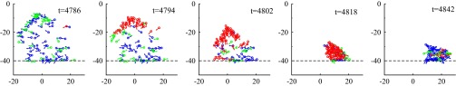
Details of a single packing event: Five consecutive snapshots are shown, taken at different time steps between $t=\mathrm{4,786}\hspace{0.17em}\text{s}$ and $t=\mathrm{4,842}\hspace{0.17em}\text{s}$. Colors encode sheep behavior according to their speed v: blue sheep are stationary, green ones are walking ($0<v\le \tilde{v}=0.41\hspace{0.17em}\text{m/s}$), and red are running $v>\tilde{v}$. Individual sheep orientations are marked by small arrows. The dashed black line marks the position of the fence. Note that the packing event is initiated by individuals far from the fence.

Fig. S5.

Second-by-second time series of (from top to bottom) the fraction $g_r$ of running sheep, the group center of mass speed $v_{cm}$, the change of the group area $\mathrm{\Delta }S$ measured over 1 s, and the mean (normalized) radial speed $v_r$. Here, time is expressed in seconds.

Individual-Based Model for Sheep Collective Behavior

To better understand the role of individual interactions in the emergence of the collective dynamics described above, we present a simple agent-based model that faithfully accounts for the observed density oscillations and the intermittency features of sheep collective dynamics.

Current models for the collective motion of animals cannot reproduce the complex avalanche dynamics highlighted by our observations. They assume that social interactions between individuals are local and can be expressed as a combination of alignment (33–35) and attraction/repulsion forces (36–38). If attraction is too weak, groups in open space are not able to maintain cohesion, and they eventually disperse in a diffusive manner. Strong enough attraction/repulsion forces, on the other hand, stabilize group size and typically yield a well-defined mean interindividual distance.

The model we present below is different. Although we do not claim that its rules are the only ones able to reproduce our experimental observations, or even that they faithfully correspond to the biological stimulus/response function of individual Merino sheep, it is useful as a proof of principle; that is, it offers insights on the kind of simple local individual interaction rules from which the sheep collective behavior may emerge. All of the rules encoded in the equations below directly follow from our observations.

Sheep Motion.

Sheep are represented by point-like agents able to perceive and respond to their local environment. The state of the ith sheep is given by its position ${\mathbf{r}}_i^t$, its heading orientation ${\theta }_i^t$, and its behavioral state $q_i^t\in \left\{\mathrm{0,1,2}\right\}$, coding, respectively, for stationary, walking, and running. Stationary sheep do not move or change their orientation, but walking and running sheeps’ position and heading evolve according to a set of Vicsek-like discrete-time equations,

$${\mathbf{r}}_i^{t+\mathrm{\Delta }t}={\mathbf{r}}_i^t+\mathrm{\Delta }t\hspace{0.17em}v\left(q_i^t\right)\hspace{0.17em}{\mathbf{s}}_i^{t+\mathrm{\Delta }t},$$ [1]

$${\theta }_i^{t+\mathrm{\Delta }t}=\mathrm{Arg}\left[{\displaystyle \sum _{j\in {\mathrm{ℳ}}_i}{\mathbf{s}}_j^t}\right]+{\psi }_i^t\left(\text{if}\hspace{0.17em}{q}_i^t=1\right),$$ [2]

$${\theta }_i^{t+\mathrm{\Delta }t}=\text{Arg}{\displaystyle \sum _{j\in {\mathcal{V}}_i}\left[{\delta }_{2,q_j^t}\hspace{0.17em}{\mathbf{s}}_j^t+\beta \hspace{0.17em}f\left(r_{ij}^t\right){\mathbf{e}}_{ij}^t\right]}\left(\text{if}\hspace{0.17em}{q}_i^t=2\right)$$ [3]

where ${\mathbf{s}}_i^t=\left(\cos {\theta }_i^t,\sin {\theta }_i^t\right)$ is the heading vector, $\mathrm{\Delta }t$ is the discrete time step, and sheep speed $v\left(q\right)$ in Eq. 1 depends on the behavioral state, $v\left(2\right)\gg v\left(1\right)>v\left(0\right)=0$. Walking sheep ($q=1$, Eq. 3) follow a classic Vicsek dynamics: Sheep i tries to align its heading with that of its metric neighbors in ${\mathrm{ℳ}}_i$, the set of all sheep closer than the interaction distance $r_0$ against a “noise” term ${\psi }_i^t$ (a random, delta-correlated angle chosen from a uniform distribution in $\left[-\eta \pi ,\eta \pi \right]$). (For simplicity, steric repulsion is not implemented explicitly here since the noise avoids individuals to stay ”on top of each other.”) Eq. 2 leads to the formation of weakly polarized local subgroups of grazing sheep that disperse diffusively in space, creating patterns similar to those observed in the experiments.

Running sheep, on the other hand, follow a more complex heading dynamics, which combines alignment interactions (with other running sheep only) with attraction/repulsion as in ref. 38: In Eq. 3, ${\mathbf{e}}_{i,j}^t$ is the unit vector oriented from sheep i to j and $f\left(r\right)=\min \left(1,\left(r-r_e\right)/r_e\right)$ is an attraction/repulsion pairwise force, with equilibrium distance $r_e$. Because packing events typically occur when sheep are widely spread out, a fixed metric interaction range is not suitable to describe the collective dynamics of running sheep. Recent results in bird flocks (19), fish schools (25), and pedestrians (39) indicate that social vertebrates interact with neighbors chosen according to “topological” (metric-free) rather than metric criteria, such as the closest k neighbors (irrespective of their distance). Here we use the first shell of Voronoi neighbors to define ${\mathcal{V}}_i$ in Eq. 3, which then contains almost always the same number of agents, independently of the local density. (See refs. 25 and 40 for details.)

Behavioral States.

We finally define the rules for the update of the behavioral state $q_i^t$, that is, the way sheep change their behavior according to local stimuli. We describe these changes by a set of transition rates between the different behavioral states. Previous experiments conducted on small groups (41, 42) have shown that the probability $p_{0\to 1}$ for a stationary individual to start walking is considerably enhanced by the presence of moving neighbors. Here, for the sake of simplicity, we ignore the weaker suppression effect of stationary neighbors and we also assume that $p_{1\to 0}$, the inverse transition, possesses the same structure, as suggested in ref. 43. Transitions rates between the stationary and the walking state are thus given as

$$p_{0\to 1}\left(i,t\right)=\frac{1+\alpha \hspace{0.17em}{n}_1^t\left(i\right)}{{\tau }_{0\to 1}},p_{1\to 0}\left(i,t\right)=\frac{1+\alpha \hspace{0.17em}{n}_0^t\left(i\right)}{{\tau }_{1\to 0}},$$ [4]

where ${\tau }_{0\to 1}$ and ${\tau }_{0\to 1}$ are spontaneous transition times, α measures the strength of mimetic effects, and $n_0^t\left(i\right)$, $n_1^t\left(i\right)$ is the number of stationary and walking metric neighbors, respectively.

The transitions to and from the running state are similar, but they depend on the number $m_R$ of running topological neighbors, with the allelomimetic effect strengthened by an exponent $\delta >1$,

$$p_{\mathrm{0,1}\to 2}\left(i,t\right)=\frac{1}{{\tau }_{\mathrm{0,1}\to 2}}{\left[\frac{{\ell }_i^t}{d_R}\left(1+\alpha \hspace{0.17em}{m}_R^t\left(i\right)\right)\right]}^{\delta }\hspace{0.17em},$$ [5]

where ${\ell }_i^t$ is the mean distance to all topological neighbors of sheep i, and $d_R$ is some characteristic length scale. The ratio between these two scales ensures that spread-out groups are much more likely to trigger a packing event than high-density ones.

Finally, for simplicity, running sheep can only transit to the stationary state with a rate $p_{2\to 0}\left(i,t\right)$ enhanced by $m_S$, the number of their stopping topological neighbors, i.e., those that switched from running to stationary in the previous time step,

$$p_{2\to 0}\left(i,t\right)=\frac{1}{{\tau }_{2\to 0}}{\left[\frac{d_S}{{\ell }_i^t}\left(1+\alpha \hspace{0.17em}{m}_S^t\left(i\right)\right)\right]}^{\delta }\hspace{0.17em},$$ [6]

where $d_S<d_R$ is a second characteristic length. The positive feedback with the stopping neighbors leads to sudden stopping of the group. Notice that now, here, ${\ell }_i$ plays a role opposite to that it had in Eq. 5: The stopping transition rate is enhanced when the topological neighbors are located at a short distance. We now briefly comment on metric and topological neighbors. Metric neighbors can be associated with the immediate surroundings of the animal and with social interactions characteristic of the grazing phase. Voronoi neighbors, on the other hand, can be thought as the first shell of individuals that can be visually perceived without obstruction from interposing sheep. Our model reflects the fact that sheep are particularly sensitive, in terms of alignment and recruitment into packing runs, to other running individuals that enter their visual range, an event that should trigger some alarm in a species subject to potential predators.

Parameter Estimation and Comparison with Experimental Data.

Many model parameters are readily given from experimental data or estimated from orders of magnitude considerations, as detailed in Agent-Based Model. In the following, we fix $v_1=0.15\hspace{0.17em}\text{m/s}$, $v_2=1.5\hspace{0.17em}\text{m/s}$, ${\tau }_{1\to 0}=8\hspace{0.17em}\text{s}$, ${\tau }_{0\to 1}=35\hspace{0.17em}\text{s}$, ${\tau }_{\mathrm{0,1}\to 2}={\tau }_{2\to 0}=N\hspace{0.17em}\text{s}$, $d_S=6.3\hspace{0.17em}\text{m}$, $d_R=31.6\hspace{0.17em}\text{m}$, $r_e=r_0=1\hspace{0.17em}\text{m}$, $\beta =0.8$ and $\eta =0.13$ (see Supporting Information for more details). This being done, we are left with two unknowns, the allelomimetic parameters α and δ. Simulations with 100 sheep reveal that dynamics similar to the one observed experimentally, with slow spreading periods followed by much shorter packing events, can be recovered only when there is a high level of imitation, namely when $\alpha >5$ and $\delta >2$.

Numerical inspection in the parameter range $\alpha \in \left[\mathrm{5,25}\right]$ and $\delta \in \left[\mathrm{2,5}\right]$ reveals that the experimental data are best described with $\alpha \simeq 15$ and $\delta \simeq 4$. Time series of the occupied surface display the same fast packing events and the typical burst pattern of $dS\left(t\right)$ (see Fig. 1B). The corresponding CCDFs match well the experimental ones (Fig. 1D). (Note that the model was simulated in open space, an additional point in favor of the negligible role of the fence in the experiments.) Movie S4 shows a typical run. The model at these optimal parameters also reproduces the intermittency of the center of mass speed $v_{cm}$ (see Fig. S6A). Cumulated over a number of events similar to that contained in the experimental data, the probability distribution function (PDF) of $v_{cm}$ shows the same noisy, possibly power-law tail with decay exponent $-2.2\left(2\right)$ (Fig. 4B), and the CDF is also compatible with the superposition of two exponentials. However, simulated over a very large number of events, power laws are ruled out, whereas the exponential fits become very good (Fig. 4C). Pending the discussion of these findings below, a general comment holds: The fact that our model is able to capture the statistical features of density fluctuations as well as the qualitative statistics of the aggregation events, with a single set of parameter values, indicates that our description captures the essential features of the stimulus–response function of individual Merino sheep.

Fig. S6.

(A) Typical time series for the center of mass speed (in minutes) for $\alpha =15$, $\delta =4$. (B–D) Three different fitness functions as a function of the allelomimetic parameters α and δ. The vertical axis is arbitrary and should not be used to compare fitness between different panels.

Fig. 4.

Model analysis for $N=100$. (A) Packing time ${\tau }_P$ (Top) and maximum group area $S_M$ (Bottom) as a function of α for different exponents δ. (B) PDF of center of mass speed $v_{cm}$ for $\alpha =15$ and $\delta =4$ obtained as in Fig. 2. Red dashed line is power-law fit with exponent $-2.2$. (C) Corresponding CCDF in lin–log scales. Red dashed lines are exponential fits with characteristic scales 0.02 and 0.08. Simulations details are given in Supporting Information.

Our main parameters α and δ both control the mean maximum group area $S_M$ reached by the group before a packing event, and the mean time ${\tau }_P$ needed to regroup to a packed configuration. Our simulations (see Fig. 4A) show that, for any $\delta >2$, ${\tau }_P$ yields a minimum as a function of α, with a global minimum located in the parameter range $\delta \in \left[\mathrm{3,4}\right]$ and $\alpha =\left[\mathrm{12,17}\right]$. $S_M$, on the other hand, does not display a global maximum, being a growing function of δ, but our chosen parameter values $\delta =4$, $\alpha =15$ seem to represent a good compromise between the competing needs discussed above. We finally note that the two-state grazing dynamics is more important than it may appear at first sight: A simpler dynamics in which all grazing sheep are walking (corresponding to the limit case ${\tau }_{1\to 0}\gg {\tau }_{0\to 1}$) produces far too spatially homogeneous configurations and does not yield a distribution of packing events consistent with the experimental data.

Discussion

We have shown that Merino sheep balance the conflicting needs of social protection and reduced competition when feeding by alternating gentle group-spreading grazing phases with fast packing events that dramatically increase the group density by up to a factor 30. Social cohesion is not reached by settling down to a steady group density but rather is maintained through sudden regroupings. Although such dynamics may be not completely unknown to field biologists, this is, to our knowledge, the first quantitative study of a large group of social herbivores in a well-controlled homogeneous feeding environment. By using homogeneous pastures, we minimize as much as possible the effect of environment heterogeneity (44). Direct predation disturbances that may be invoked to explain increases in group density (12, 13, 45) are also ruled out in this context. Therefore, we are able to argue that this collective behavior mainly results from socially driven individual decisions.

The combination of experimental analyses with the numerical study of a spatially explicit model offers insights on the individual-level stimulus/response functions that can underlie such complex collective phenomena. In particular, our work points to a local origin for packing events: Danger/fear increases with the typical distance to visual/topological neighbors, up to a threshold beyond which running is triggered. A few sheep initiate a wave of recruitment into a running (sub) group, in agreement with earlier observations that vigilance is increased for individuals at the edge of a group (46, 47). Our model shows that local but metric-free interactions, together with strong allelomimetic behavior, are sufficient to generate such complex collective intermittent dynamics. Its main free parameters, α and δ, quantify the gregarious character of our sheep. That they must be chosen with large numerical values to reproduce experimental observations is a measure of the strong allelomimetic behavior of Merino sheep. In this parameter range, spotting a single running individual is often enough to induce a run in other sheep, surely a useful trait in a social animal subjected to predation risks. Moreover, we have shown that these parameter values offer a reasonable compromise between the need to cover a large grazing area and to minimize the time to regroup. Thus, one may conjecture that the ability of sheep to maintain cohesion through such self-organized density oscillations could be linked to a behavioral optimization process within a social context. Such an optimization process could have tuned the strength of allelomimetic interactions between sheep so as to ensure, at the individual scale, a fine balance between (i) the need to explore the maximum area of space to avoid interindividual competition when foraging and (ii) the need to keep contact with the other group members to ensure cohesion and protection.

Given the elementary nature of the decision-making rules studied here, it is likely that the same phenomenon is present in other social species (48) whenever imperatives for mutual protection and foraging/exploration compete.

We finally discuss the statistics of packing events. Both experiments and model show that they are distributed over all accessible scales. The precise functional form of this distribution remains unclear: A power-law tail remains possible for the field data but is excluded for the model data, which are best accounted for by the superposition of two exponentials. It is thus difficult to decide between two alternatives for the field data: Either they do exhibit power-law behavior (albeit with a decay exponent leading to a well-defined mean event size) and the model is incomplete or they are also best described by the superposition of several exponentials. Further data, especially on larger groups, would thus be highly desirable to shed more light on this point. Note that, to invoke a true self-organized criticality scenario (49), the timescales separation inherent to the behavioral mechanisms described here should likely grow with group size. On the other hand, it has been recently argued that some animal groups, although not truly critical in the rigorous sense, might operate at the maximally critical regime allowed by their (ineluctably) finite size (50).

At any rate, this may be of little biological importance: For all practical purposes, the large sheep herds studied here show the ability to fluctuate and respond fast on a wide range of scales, in line with the general idea that certain biological systems operate in some self-organized, marginally stable regime.

Materials and Methods

Study Area, Subjects, and Experimental Design.

Fieldwork was carried out at the experimental farm of Domaine du Merle (5.74°E and 48.50°N) in the south of France, from November 2008 to January 2009. This station, located in the Crau region, raises Merinos d’Arles sheep in native or irrigated pasture. Wild and domestic sheep (Ovis sp.) are gregarious species that live in open-membership groups, and merino sheep is reputed to be one of the most gregarious among domestic breeds (30). Therefore, it represents an ideal species to unravel mechanisms involved in cohesion and collective patterns.

To quantify the interactions between individuals and limit the influence of external factors, we used same-age groups with standardized conditions in term of sex (only females) and pastures (flat and homogeneous irrigated native pasture of the Crau region). For the November 2008 fieldwork, we randomly selected 200 unrelated 18-mo-old females from a larger flock of 1,600 sheep. The experiments were carried out in flat and homogeneous irrigated native pastures. The experimental setup consisted of four adjacent 80 × 80 m enclosures, delimited by sheep fences, each with an associated waiting area. Green polypropylene 1.2-m-high net was used to visually isolate sheep from the immediate surroundings and from other enclosures. A 7-m-high tower placed in the center of the setup was used to register the position of sheep (see Fig. S1).

During the experimental days, the herds were led from their night enclosure within the waiting enclosure area, where they remained before introduction in the adjacent enclosure, until the digital camera was secured to the top of the observation tower and ready to take snapshots. Experiments begun first by simultaneously introducing two sheep groups, each one composed by 100 18-mo-old sheep, in two different and separated enclosures. The two groups of 100 sheep were simultaneously recorded (see below) while grazing freely for 1 h. The same protocol was duplicated the following morning. After a series of experiments conducted with smaller groups within the same enclosures (which will be the subject of a different work), we performed two additional experiments in January 2009, this time selecting 100 3.5-y-old sheep and using a single 80 × 80 m enclosure plus waiting area. The first experiment had again the time length of 1 h, whereas the second lasted for ∼3.5 h.

All experiments conducted with groups of 100 sheep began at 0930 hours. Animal care and experimental manipulations were applied in conformity with the rules of the Ethics Committee for Animal Experimentation of Federation of Research in Biology of Toulouse.

Data Collection and Tracking.

An observation tower was positioned at the corner of the enclosures. Digital cameras (15.1-megapixel Canon EOS D50) were anchored on the top of the tower, at 7.50 m height. Frames were taken with a temporal resolution of one image per second. Automatic sheep detection and tracking from field snapshots was impossible because of major changes of exposure that caused the contrast between sheep and background to fluctuate a lot, and angle of view means that sheep frequently hide each other from the camera viewpoint. Therefore, we had to resort to manual tracking on a Cintiq interactive pen display [Cintiq 21 UX (UXGA 1,600 × 1,200 pixels)] using dedicated software written by J. Gautrais. The positions ${\mathbf{r}}_i^t$ and headings ${\mathbf{s}}_i^t$ were obtained by manually marking in the digital pictures the hind and head positions of each sheep i. With a typical sheep size of around 1 m, we can give a conservative estimate of the positional tracking error $\mathrm{\Delta }r$ due to manual tracking of around 20$\text{\%}$ of sheep size, or $\mathrm{\Delta }r\approx 0.2\hspace{0.17em}\text{m}$.

By marking each sheep in two consecutive pictures, we have been able to track sheep movement from one image to the next, reconstructing sheep velocities as ${\mathbf{v}}_i^t=\left({\mathbf{r}}_i^{t+\mathrm{\Delta }t}-{\mathbf{r}}_i^t\right)/\mathrm{\Delta }t$.

Note that, in our manual tracking procedure, we chose to track one sheep at a time over the two consecutive frames. Our dedicated software allows one to import by default the marked hind and head position from one frame to the following, with the option to manually correct them if the sheep has moved between the two frames. Therefore, positional tracking errors $\mathrm{\Delta }r$ between consecutive-in-time sheep positions are strongly correlated for slow-moving sheep and completely correlated for stationary sheep. This implies that stationary (${\mathbf{v}}_i^t=0$) sheep were detected with almost no error and that, in general, errors on velocity measures tend to grow for increasing speed. Assuming uncorrelated errors, we can estimate the maximum error on sheep speed as

$$\mathrm{\Delta }v=\frac{\sqrt{2}\mathrm{\Delta }r}{\mathrm{\Delta }t}\approx 0.3\text{m}/\text{s}.$$ [S1]

Our dedicated software makes use of projective geometry techniques to convert the manual marking in the camera pixel coordinate system into absolute coordinates on the experimental field plane, as detailed in Field Positions Reconstruction. To do so, four different reference points are needed to calibrate the coordinate transformation. To this end, four 0.3 × 0.3 m 1-m-high panels were placed at each corner of the square enclosures for the whole duration of experiments to be used as reference points (see Fig. S1). The accuracy of their locations has been verified by cross-checking the length and orthogonality of diagonals with 1-cm-precision GPS devices. Our check indicates that the positional accuracy was less than 10 cm.

Due to the large amount of manual work required to process the entire 3.5-h sequence second by second, we chose a sampling rate of 1 min to extract sheep positions, headings, and velocities (thus we actually processed two snapshots per minute). As seen in the following, this sampling rate is significantly smaller than the typical autocorrelation time that characterizes the collective aggregation phenomena, so that we expect that no significant information is lost due to our sampling choice. As discussed in Experimental Results, we have also performed a complete tracking—with the maximum sampling rate of one second—of a single packing event taking place during the 3.5-h-long dataset.

Additional Data Analysis

In this section, we further discuss experimental data analysis and present some additional data not shown in the main text. Our tracking time extends over 3 h and 30 min, during which we manually tracked sheep positions, orientations, and velocity every 60 s. Due to the difficulties of tracking individual sheep that are partially or totally covered by other members of the herd, even manual tracking is not always 100% successful. The tracking error rate (percentage of nontracked sheep) per each frame is reported in Fig. S2A. The large tracking error spike, just after $t=100$ min, is associated with a large packing event in which the entire herd rushed quite quickly across the field (roughly from top left to bottom right) in a tightly packed configuration. The relatively high tracking error rate experienced toward the end of the session, on the other hand, is due to the group being located near the top right corner of the field, the farthest from our observation point. In general, it should be remarked that the inability to track a minority of sheep in tightly packed configuration does not affect significantly the averaged quantities like the group-covered surface or the center of mass speed. Missed individuals, in fact, are in close contact with the tracked ones, and exhibit similar behaviors in terms of velocity. Outlier individuals, which move with different velocities or are significantly remote from the tight group, in fact, are easily tracked manually, and are not missed by our analysis.

For completeness, in Fig. S2B, we report the magnitude of the macroscopic polarization ${\mathbf{P}}^t={\langle {\mathbf{s}}_i^t\rangle }_i$ time series. It shows moderate correlation with the indicator of packing events, such as the center of mass speed $v_{cm}$ (correlation coefficient $c=0.2$, with a P value $p=0.004$) or the change in the group area $dS$ ($c=-0.15$, $p=0.036$). Here and in the main text, P values for correlation coefficients are computed as the probability that two random permutations of the time series analyzed are more correlated (or anticorrelated) than the original time series.

Another interesting quantity in the study of the slow spreading/fast packing collective dynamics is the herd center of mass displacement, either measured during the packing events or in the intervening spreading phases. They are both displayed in Fig. S3A as a function of the packing or spreading phase duration. It is clear that, during both phases, the sheep group can travel over up to almost half the arena linear size. Although our time resolution of 1 min prevents any accurate estimation (especially for the shortest packing events), it is clear that the herd seems to displace more quickly during the packing phase (red dots in Fig. S3A). Notice also that the spreading phase (green squares) seems to be characterized by a finite displacement velocity, in agreement with the nonzero mean polarization exhibited by the herd in Fig. S2B.

Following the wide distribution of packing event sizes discussed in the main text, one is naturally led to also consider the statistics of the group area $S_M$ and of its variation $dS$. In Fig. S3B, we report the CCDFs for both S and $dS$, showing that they are characterized by a well-defined scale.

Fig. S4 reports the (normalized) speed distribution $P\left(v\right)$ of the instantaneous speed $v_i^t=\left|{\mathbf{v}}_i^t\right|$, computed over all moving ($q_i=\mathrm{1,2}$) sheep i and all tracked time steps t. (For practical reasons, we defined moving sheep as all sheep with a speed larger than ${10}^{-2}\text{m}/\text{s}$.) The resulting speed distribution may be seen as the sum of two separate distributions. The first distribution originates from sheep walking at low speed and may be fitted by a Poissonian function $F_1\left(v\right)=a_{0}v\exp \left(-v/a_1\right)$. The second one, well captured by a skewed Gaussian distribution $F_2\left(v\right)=b_{0}v\exp \left[-{\left(v-b_1\right)}^2/2b_2^2\right]$, describes the fast-running sheep. The best fitting parameters are $a_0=61.4,a_1=0.10$ and $b_0=1.1,b_1=0.22,b_2=0.48$. We can define a speed threshold $\tilde{v}$ separating high from low speed by the condition $F_1\left(\tilde{v}\right)=F_2\left(\tilde{v}\right)$, which gives $\tilde{v}\approx 0.41\hspace{0.17em}\text{m}/\text{s}$. Therefore, at each time step, a sheep can be assigned one of the three behavioral states according to its instantaneous velocity: stationary when its speed is zero, walking when $0<v_i^t<\tilde{v}$, and running when $v_i^t>\tilde{v}$.

Sheep changed their speed/state frequently across time, and relevant quantities in our analyses are the instantaneous fraction of stationary, walking, and running sheep, respectively $g_s^t$, $g_w^t$, and $g_r^t\in \left[\mathrm{0,1}\right]$. By averaging them over all tracked time steps, we have ${\langle g_s^t\rangle }_t\approx 0.74$, ${\langle g_w^t\rangle }_t\approx 0.17$, and ${\langle g_r^t\rangle }_t\approx 0.09$. The mean speed of walking sheep is thus $0.18\hspace{0.17em}\text{m}/\text{s}$, whereas, for running sheep, we have a mean speed of $0.76\hspace{0.17em}\text{m/s}$.

The fraction of running individuals $g_r^t$ is strongly correlated with the center of mass speed $v_{cm}^t$ (the Pearson correlation coefficient between the two indicators is $c=0.95$, with a P value $\text{<}{10}^{-6}$), and shows the same intermittency behavior exhibited by the group center of mass speed, as can be seen in Fig. S4. To test the resilience of $g_r^t$ on the threshold $\tilde{v}$ used to define a running individual, we also tested thresholds different from $\tilde{v}=0.41\hspace{0.17em}\text{m/s}$. As shown in Fig. S4, the corresponding CCDFs show essentially the same behavior in the range $v=\tilde{v}\pm 0.1$. The time series for the fractions of walking and stationary individuals show no significant features and are not shown here.

Finally, in Fig. S5, we report the second-by-second time series of several dynamical descriptors measured during the single packing event discussed in the main text. From top to bottom, we show the fraction $g_r$ of running sheep, the group center of mass speed $v_{cm}$, the change of the group area $\mathrm{\Delta }S$ measured over 1 s, and the mean (normalized) radial speed

$$v_r^t\equiv \langle \left[\left({\mathbf{r}}_i^t-{\mathbf{r}}_{cm}^t\right)\cdot {\mathbf{v}}_i^t\right]/\left[\Vert \left({\mathbf{r}}_i^t-{\mathbf{r}}_{cm}^t\right)\Vert \Vert {\mathbf{v}}_i^t\Vert \right]\rangle ,$$ [S2]

where ${\mathbf{r}}_{cm}^t$ is the center of mass position and $\langle \cdot \rangle$ denotes the average over all sheep. Negative values of $v_r$ signal the tendency of individual sheep to move toward the group center of mass. All these indicators are obviously correlated along the packing event.

Individual-Based Model

In this section, we provide further details on the numerical analysis of our agent-based model. The dynamics is discrete in time, with synchronous updates. In a discrete time model with time step $\mathrm{\Delta }t$, the switching rate p defined by Eqs. 4–6 translates to switching probabilities $P=1-e^{-p\mathrm{\Delta }t}$, which control the behavioral state transitions $q_i^t\to q_i^{t+\mathrm{\Delta }t}$ over one time step. We have chosen a time step $\mathrm{\Delta }t=1\hspace{0.17em}\text{s}$, which coincides with our maximum experimental sampling rate.

Numerical simulations have been performed with groups of $N=100$ individuals in open space, starting from a tightly grouped configuration of stationary and strongly polarized sheep. A finite size analysis is left for future investigations. To study the stationary regime of our model, in all our numerical simulations, we have first discarded a long (${10}^5$ time steps) transient before performing any analysis of model behavior.

Parameter Estimation.

Many parameters of the model can be deduced from experimental data or fixed by order of magnitude considerations. The walking and running speeds are, respectively, of the order of $v\left(1\right)\sim 0.1\hspace{0.17em}\text{m/s}$ and $v\left(2\right)\sim 1\hspace{0.17em}\text{m/s}$ (see Fig. S4A). Both the metric interaction range $r_0$ and $r_e$, the equilibrium distance of the two-body force between running sheep, can be assumed to be of the order of magnitude of one sheep body length, thus of the order of 1 m.

For the grazing dynamics, the ratio between the spontaneous switching times ${\tau }_{0\to 1}$ and ${\tau }_{1\to 0}$ roughly fixes the proportion between stationary and walking sheep. According to our field data, one has ${\tau }_{0\to 1}/{\tau }_{1\to 0}\approx 74/17\approx 4.4$. Moreover, sheep usually keep walking for several seconds before stopping, so that we estimate ${\tau }_{1\to 0}$ to be of the order of 10 s.

Determining the parameter values involved in the switching rates $p_{\mathrm{0,1}\to 2}$ and $p_{2\to 0}$ is not so straightforward, but it is reasonable to assume that the ratio between the length scales $d_R$ and $d_S$ is roughly proportional to the square root of the ratio between the maximum and the minimum group area, which our field observations set roughly at 30; that is, $d_R\approx 5d_S$. Note that although the amplitude of group surface oscillations generically increases with $d_S$, due to the complex and spatially inhomogeneous dynamics, the relation is not a trivial one.

Finally, we estimate the timescales ${\tau }_{\mathrm{0,1}\to 2}$ and ${\tau }_{2\to 0}$ by imposing that the corresponding switching rates $p\sim 1/N$ when ${\ell }_i=d_R,d_S$, yielding ${\tau }_{\mathrm{0,1}\to 2}={\tau }_{2\to 0}\sim N$. This choice means that one expects a single spontaneous switch per unit time when the entire group reaches the dilution level fixed by the length scales $d_R,d_S$. Note that this is a very rough, mean-field-like estimate, because highly diluted groups are not homogeneous.

Numerical Simulations.

To compare our numerical results with experimental data, we have first analyzed our model dynamics over a timespan comparable with the length of experimental time series (after discarding the transient defined above). We use the above estimations to constrain a priori the majority of model parameters, thus vastly reducing the parameter space. After a preliminary exploration, where we mainly tried to qualitatively reproduce the spatial and temporal scales of the group area $S\left(t\right)$ (see main text) oscillations, and to discard parameter values that may lead to “exotic states” never observed on the field, we fixed the majority of model parameters as follows: $v_1=0.15\hspace{0.17em}\text{m/s}$, $v_2=1.5\hspace{0.17em}\text{m/s}$, $\beta =0.8$, ${\tau }_{1\to 0}=8\hspace{0.17em}\text{s}$, ${\tau }_{0\to 1}=35\hspace{0.17em}\text{s}$, ${\tau }_{\mathrm{0,1}\to 2}={\tau }_{2\to 0}=N\hspace{0.17em}\text{s}$, $r_e=r_0=1\hspace{0.17em}\text{m}$, and $d_R=5\hspace{0.17em}{d}_S$, with the noise amplitude constrained in the range $\eta \in \left[0.1,0.5\right]$ and the allelomimetic parameters $\delta >2$, $\alpha >5$. (Some extreme parameter values, like a too high cohesion β, for instance, may lead to metastable states, in which a group of running sheep moves back and forth between two distinct groups of stationary and tightly packed individuals.)

The noise amplitude essentially controls the diffusive spreading of individuals during the grazing phase, and, in the following, we fixed it to $\eta =0.13$. We also set the stopping characteristic length scale (see Eq. 6) $d_S=6.3$ m, a value that nicely fits the experimentally observed group minimal extension.

This preliminary analysis left us with only two free parameters, the allelomimetic coefficients δ and α, which have been subsequently carefully explored in the ranges $\delta \in \left[\mathrm{2,5}\right]$, $\alpha \in \left[\mathrm{5,25}\right]$.

Relatively short runs, of about 13,000 time steps after the transient, were analyzed for direct comparison with the experimental time series (which have the same length) for the group area and its center of mass speed. We obtained an optimal agreement, both for the time series and their corresponding probability distributions for values close to $\delta \approx 4$ and $\alpha \approx 15$. The data shown in Figs. 1 B–D and 4 B and C, have indeed been obtained with the exact values $\delta =4$ and $\alpha =15$. A typical time series for the center of mass speed $v_{CM}$ is shown in Fig. S6A.

To evaluate the mean maximum group area $S_M$ and the mean packing time ${\tau }_P$, on the other hand, we have performed longer runs (of the order of ${10}^5$ time steps after transient), and extracted the average values as a function of α and δ. More precisely, $S_M$ is the average value of the local maxima exhibited by the $S\left(t\right)$ time series, and ${\tau }_P$ is the average time needed for the group to pass from one local maximum to the next local minimum*. The resulting mean values $S_M$ and ${\tau }_P$ are reported in Fig. 4A for integer values of δ, but we have also explored half-integer δ values (which are not shown, to avoid overcrowding).

Fitness Function.

Once we have computed these mean values, it is tempting to combine them to extract some kind of fitness function. As discussed in the main text, one is naturally led to hypothesize that individual fitness decreases with ${\tau }_P$ and increases with $S_M$, leading to a fitness function $F\left(S_M,{\tau }_P\right)$ that grows with $S_M$ and decreases with ${\tau }_P$. Any such combination, however, is largely arbitrary in the absence of further input from biological data, especially because it is not possible to form any dimensionless combination out of $S_M$ (an area) and ${\tau }_P$, a time.

We have nevertheless tried a few combinations as a largely speculative attempt at exploring this issue. The first is simply $F_1=S_M/{\tau }_P$, and, as shown in Fig. S6B, it is dominated by $S_M$, which grows constantly with the allelomimetic exponent δ. One can argue that the utility of a large grazing area for a finite group of sheep should eventually saturate, as the per capita available area for grazing reaches a value that guarantees optimal foraging for each individual. One is therefore led to discard this choice. The second choice (shown in Fig. S6C) directly compares a distance (actually $\sqrt{S}$ is a proxy for the mean distance neighboring sheep) with a time, $F_2=\sqrt{S_M}/{\tau }_P$, and shows sign of a saturation toward a maximum value for $\delta \in \left[\mathrm{4,5}\right]$ and $\alpha \in \left[\mathrm{10,15}\right]$. The third choice, finally, has the somehow more complicated form $F_3=\sqrt{S_M}/{\tau }_P^2$, but shows a clear maximum value for $\delta =3.5$ and $\alpha =14$ (Fig. S6D). Altogether, the two latter choices seems to be optimized in an allelomimetic parameter range significantly close to the actual values that faithfully reproduce field observations.

Field Positions Reconstruction: The Projective Geometric Mapping

During the data acquisition, it was not possible to fix the camera on the tower with an exact position and orientation between consecutive days. Hence, the classical true perspective projection (i.e., the pinhole camera model) to get sheep positions out of the 2D images could not be used, and we resorted to projective geometry mapping (51). The projective plane intends to model the geometric properties of the perspective projection. A point in the projective plane is represented by three homogeneous coordinates, say $\left(x,y,z\right)$, instead of the two conventional Cartesian coordinates, say $\left(u,v\right)$. The relationship between both representations is merely

$$\{\begin{array}{c}u=\frac{x}{z}\\ v=\frac{y}{z}\end{array}.$$ [S3]

Of course, any homogeneous coordinate dilation $\left(\lambda x,\lambda y,\lambda z\right)$ will project to the same Cartesian point $\left(u,v\right)$ as $\left(x,y,z\right)$. This is the basic property of perspective projection: Every point on the ray connecting $\left(u,v\right)$ and the center of projection collapses to the same projected point, namely $\left(u,v\right)$ itself. This makes it possible to express the projective transformation of the projective planes as a simple 3 × 3 matrix product of respective homogeneous coordinates. Because the overall scale factor does not affect Cartesian coordinates, one of the matrix coefficients can safely be set arbitrarily to 1; hence the matrix has eight essential parameters. We define the camera coordinates system $\left(u,v\right)$ following the pixel coordinates: $\left(\mathrm{0,0}\right)$ at the top left pixel and axis following the pixels array indexes. We define the field coordinates system with the center of the paddock, x axis along the horizon and y axis accordingly (Fig. S1). The mapping between the two systems reads

$$\left(\begin{array}{c}ku\\ kv\\ k\end{array}\right)=\left(\begin{array}{ccc}{t}_1& t_2& t_3\\ t_4& t_5& t_6\\ t_7& t_8& 1\end{array}\right)\left(\begin{array}{c}X\\ Y\\ Z\end{array}\right)$$ [S4]

where $\left(u,v\right)$ are the pixel indexes of the points $\left(x=X/Z,y=Y/Z\right)$ in field coordinates. The $t_i$ are the parameters that uniquely define the transformation from field coordinates to pixel coordinates, following

$$\{\begin{array}{c}u=\frac{ku}{k}=\frac{t_{1}x+t_{2}y+t_3}{t_{7}x+t_{8}y+1}\\ v=\frac{kv}{k}=\frac{t_{4}x+t_{5}y+t_6}{t_{7}x+t_{8}y+1}\end{array}.$$ [S5]

To determine the eight $t_i$ values, we need eight equations, i.e., four reference points in the field $P_i=\left(x_i,y_i\right),\hspace{0.17em}i=\mathrm{1..4}$ for which we know the corresponding pixel coordinates $\left(u_i,v_i\right)$. We then have

$$\left(\begin{array}{cccccccc}{x}_1& y_1& 1& 0& 0& 0& -u_1{x}_1& -u_1{y}_1\\ 0& 0& 0& x_1& y_1& 1& -v_1{x}_1& -v_1{y}_1\\ x_2& y_2& 1& 0& 0& 0& -u_2{x}_2& -u_2{y}_2\\ 0& 0& 0& x_2& y_2& 1& -v_2{x}_2& -v_2{y}_2\\ x_3& y_3& 1& 0& 0& 0& -u_3{x}_3& -u_3{y}_3\\ 0& 0& 0& x_3& y_3& 1& -v_3{x}_3& -v_3{y}_3\\ x_4& y_4& 1& 0& 0& 0& -u_4{x}_4& -u_4{y}_4\\ 0& 0& 0& x_4& y_4& 1& -v_4{x}_4& -v_4{y}_4\end{array}\right)\left(\begin{array}{c}{t}_1\\ t_2\\ t_3\\ t_4\\ t_5\\ t_6\\ t_7\\ t_8\end{array}\right)=\left(\begin{array}{c}{u}_1\\ v_1\\ u_2\\ v_2\\ u_3\\ v_3\\ u_4\\ v_4\end{array}\right).$$ [S6]

In the field setup, four 0.3 × 0.3 m panels were put at each corner of the square enclosures for the whole duration of experiments to obtain the reference points, which are positions defining an orthonormal coordinate system (Fig. S1). The accuracy of the locations were estimated by cross-checking distances and orthogonality of diagonals. An a posteriori control using 1-cm precision GPS devices ⁴ indicates that the positional accuracy was less than 10 cm. (The SR20 single frequency survey system performs high-accuracy static and kinematic data collection for the land surveyor.) Because the square side length was $80$ m, the field coordinates of the four reference points $P_1\dots P_4$ were then

$$\begin{array}{c}{P}_1=\left(R,0\right)\\ P_2=\left(0,R\right)\\ P_3=\left(-R,0\right)\\ P_4=\left(0,-R\right)\end{array}$$ [S7]

with $R=40\sqrt{2}$ m, which can be plug into Eq. S6. (For easiness of representation, in the main text, we have rotated this coordinate system by ${45}^{\text{o}}$.)

A solution for the $t_i$ is then obtained by

$$\begin{array}{c}{t}_8=\frac{1}{R}\frac{\left(v_4+v_2-v_1-v_3\right)\left(u_2-u_4\right)-\left(u_4+u_2-u_1-u_3\right)\left(v_2-v_4\right)}{\left(v_3-v_1\right)\left(u_2-u_4\right)-\left(u_3-u_1\right)\left(v_2-v_4\right)}\\ t_7=\frac{1}{R}\frac{\left(v_4+v_2-v_1-v_3\right)\left(u_3-u_1\right)-\left(u_4+u_2-u_1-u_3\right)\left(v_3-v_1\right)}{\left(v_4-v_2\right)\left(u_1-u_3\right)-\left(u_4-u_2\right)\left(v_1-v_3\right)}\\ t_5=\frac{1}{2R}\left(v_3-v_1+R\left(v_1+v_3\right)t_8\right)\\ t_2=\frac{1}{2R}\left(u_3-u_1+R\left(u_1+u_3\right)t_8\right)\\ t_1=\frac{1}{R}\left(\left(u_2-u_1\right)+R{u}_1{t}_8-R{u}_2{t}_7-R{t}_2\right)\\ t_4=\frac{1}{R}\left(\left(v_2-v_1\right)+R{v}_1{t}_8-R{v}_2{t}_7-R{t}_5\right)\\ t_3=u_1-R{u}_1{t}_8+R{t}_2\\ t_6=v_1-R{v}_1{t}_8+R{t}_5\end{array}.$$ [S8]

Finally, for any point P of pixel coordinates $\left(u,v\right)$, we obtain its corresponding field coordinates $\left(x,y\right)$ following

$$\begin{array}{c}det=\left(t_{8}v-t_5\right)\left(t_{7}u-t_1\right)-\left(t_{8}u-t_2\right)\left(t_{7}v-t_4\right)\\ x=\left(\left(t_{8}v-t_5\right)\left(t_3-u\right)-\left(t_{8}u-t_2\right)\left(t_6-v\right)\right)/det\\ y=\left(\left(t_{7}u-t_1\right)\left(t_6-v\right)-\left(t_{7}v-t_4\right)\left(t_3-u\right)\right)/det\end{array}.$$ [S9]

References

- 1.Partridge BL, Johansson J, Kalish J. The structure of schools of giant bluefin tuna in Cape Cod Bay. Environ Biol Fishes. 1983;9(3-4):253–262. [Google Scholar]
- 2.Bednarz JC. Cooperative hunting Harris’ hawks (Parabuteo unicinctus) Science. 1988;239(4847):1525–1527. doi: 10.1126/science.239.4847.1525. [DOI] [PubMed] [Google Scholar]
- 3.Creel S, Creel NM. Communal hunting and pack size in African wild dogs, Lycaon pictus. Anim Behav. 1995;50(5):1325–1339. [Google Scholar]
- 4.Handegard NO, et al. The dynamics of coordinated group hunting and collective information transfer among schooling prey. Curr Biol. 2012;22(13):1213–1217. doi: 10.1016/j.cub.2012.04.050. [DOI] [PubMed] [Google Scholar]
- 5.Deneubourg JL, Goss S. Collective patterns and decision making. Ethol Ecol Evol. 1989;1(4):295–311. [Google Scholar]
- 6.Seeley TD. Honeybee Democracy. Princeton Univ Press; Princeton, NJ: 2010. [Google Scholar]
- 7.Ballerini M, et al. Empirical investigation of starling flocks: A benchmark study in collective animal behaviour. Anim Behav. 2008;76(1):201–215. [Google Scholar]
- 8.Foster WA, Treherne JE. Evidence for the dilution effect in the selfish herd from fish predation on a marine insect. Nature. 1981;293:466–467. [Google Scholar]
- 9.Treherne JE, Foster WA. Group transmission of predator avoidance-behavior in a marine insect: The Trafalgar effect. Anim Behav. 1981;29(3):911–917. [Google Scholar]
- 10.Domenici P, Batty RS. Escape behaviour of solitary herring (Clupea harengus) and comparisons with schooling individuals. Mar Biol. 1997;128(1):29–38. [Google Scholar]
- 11.Domenici P, Standen EM, Levine RP. Escape manoeuvres in the spiny dogfish (Squalus acanthias) J Exp Biol. 2004;207(Pt 13):2339–2349. doi: 10.1242/jeb.01015. [DOI] [PubMed] [Google Scholar]
- 12.Procaccini A, et al. Propagating waves in starling, Sturnus vulgaris, flocks under predation. Anim Behav. 2011;82(4):759–765. [Google Scholar]
- 13.King AJ, et al. 2012. Selfish-herd behaviour of sheep under threat. Curr Biol 22(14): R561–R562.
- 14.Giardina I. Collective behavior in animal groups: Theoretical models and empirical studies. HFSP J. 2008;2(4):205–219. doi: 10.2976/1.2961038. [DOI] [PMC free article] [PubMed] [Google Scholar]
- 15.Vicsek T, Zafeiris A. Collective motion. Phys Rep. 2012;517(3-4):71–140. [Google Scholar]
- 16.Camazine S, et al. Self-Organization in Biological Systems. Princeton Univ Press; Princeton, NJ: 2001. [Google Scholar]
- 17.Krause J, Ruxton GD. Living in Groups. Oxford Univ Press; Oxford: 2002. [Google Scholar]
- 18.Sumpter DJ. Collective Animal Behavior. Princeton Univ Press; Princeton, NJ: 2010. [Google Scholar]
- 19.Ballerini M, et al. Interaction ruling animal collective behavior depends on topological rather than metric distance: Evidence from a field study. Proc Natl Acad Sci USA. 2008;105(4):1232–1237. doi: 10.1073/pnas.0711437105. [DOI] [PMC free article] [PubMed] [Google Scholar]
- 20.Buhl J, Sword GA, Simpson SJ. Using field data to test locust migratory band collective movement models. Interface Focus. 2012;2(6):757–763. doi: 10.1098/rsfs.2012.0024. [DOI] [PMC free article] [PubMed] [Google Scholar]
- 21.Attanasi A, et al. Collective behaviour without collective order in wild swarms of midges. PLOS Comput Biol. 2014;10(7):e1003697. doi: 10.1371/journal.pcbi.1003697. [DOI] [PMC free article] [PubMed] [Google Scholar]
- 22.Cavagna A, et al. Scale-free correlations in starling flocks. Proc Natl Acad Sci USA. 2010;107(26):11865–11870. doi: 10.1073/pnas.1005766107. [DOI] [PMC free article] [PubMed] [Google Scholar]
- 23.Katz Y, Tunstrøm K, Ioannou CC, Huepe C, Couzin ID. Inferring the structure and dynamics of interactions in schooling fish. Proc Natl Acad Sci USA. 2011;108(46):18720–18725. doi: 10.1073/pnas.1107583108. [DOI] [PMC free article] [PubMed] [Google Scholar]
- 24.Herbert-Read JE, et al. Inferring the rules of interaction of shoaling fish. Proc Natl Acad Sci USA. 2011;108(46):18726–18731. doi: 10.1073/pnas.1109355108. [DOI] [PMC free article] [PubMed] [Google Scholar]
- 25.Gautrais J, et al. Deciphering interactions in moving animal groups. PLos Comput. Biol. 2012;8(9):e1002678. doi: 10.1371/journal.pcbi.1002678. [DOI] [PMC free article] [PubMed] [Google Scholar]
- 26.Puckett JG, Kelley DH, Ouellette NT. Searching for effective forces in laboratory insect swarms. Sci Rep. 2014;4:4766. doi: 10.1038/srep04766. [DOI] [PMC free article] [PubMed] [Google Scholar]
- 27.Becco C, Vanderwalle N, Delcourt J, Poncin P. Experimental evidences of a structural and dynamical transition in fish school. Physica A. 2006;367:487–493. [Google Scholar]
- 28.Tunstrøm K, et al. Collective states, multistability and transitional behavior in schooling fish. PLOS Comput Biol. 2013;9(2):e1002915. doi: 10.1371/journal.pcbi.1002915. [DOI] [PMC free article] [PubMed] [Google Scholar]
- 29.Hunter JR. Swimming and feeding behavior of larval anchovy Engraulis mordax. Fish Bull. 1972;70:821–838. [Google Scholar]
- 30.Hamner WM. Aspects of schooling in Euphausia superba. J Crustac Biol. 1984;4:67–74. [Google Scholar]
- 31.Arnold GW, Dudzinski ML. The Ethology of Free-Ranging Domestic Animals. Elsevier; Amsterdam: 1978. [Google Scholar]
- 32.Attanasi A, et al. Information transfer and behavioural inertia in starling flocks. Nat Phys. 2014;10(9):615–698. doi: 10.1038/nphys3035. [DOI] [PMC free article] [PubMed] [Google Scholar]
- 33.Vicsek T, Czirók A, Ben-Jacob E, Cohen I, Shochet O. Novel type of phase transition in a system of self-driven particles. Phys Rev Lett. 1995;75(6):1226–1229. doi: 10.1103/PhysRevLett.75.1226. [DOI] [PubMed] [Google Scholar]
- 34.Grégoire G, Chaté H. Onset of collective and cohesive motion. Phys Rev Lett. 2004;92(2):025702. doi: 10.1103/PhysRevLett.92.025702. [DOI] [PubMed] [Google Scholar]
- 35.Chaté H, Ginelli F, Grégoire G, Raynaud F. Collective motion of self-propelled particles interacting without cohesion. Phys Rev E Stat Nonlin Soft Matter Phys. 2008;77(4 Pt 2):046113. doi: 10.1103/PhysRevE.77.046113. [DOI] [PubMed] [Google Scholar]
- 36.Reynolds C. Flocks, herds and schools: A distributed behavioral model. Comput Graph. 1987;21(4):25–34. [Google Scholar]
- 37.Couzin ID, Krause J, James R, Ruxton GD, Franks NR. Collective memory and spatial sorting in animal groups. J Theor Biol. 2002;218(1):1–11. doi: 10.1006/jtbi.2002.3065. [DOI] [PubMed] [Google Scholar]
- 38.Grégoire G, Chaté H, Tu Y. Moving and staying together without a leader. Phys D. 2003;181(3-4):157–170. [Google Scholar]
- 39.Moussaïd M, Helbing D, Theraulaz G. How simple rules determine pedestrian behavior and crowd disasters. Proc Natl Acad Sci USA. 2011;108(17):6884–6888. doi: 10.1073/pnas.1016507108. [DOI] [PMC free article] [PubMed] [Google Scholar]
- 40.Ginelli F, Chaté H. Relevance of metric-free interactions in flocking phenomena. Phys Rev Lett. 2010;105(16):168103. doi: 10.1103/PhysRevLett.105.168103. [DOI] [PubMed] [Google Scholar]
- 41.Pillot MH, et al. Scalable rules for coherent group motion in a gregarious vertebrate. PLoS One. 2011;6(1):e14487. doi: 10.1371/journal.pone.0014487. [DOI] [PMC free article] [PubMed] [Google Scholar]
- 42.Ramseyer A, Boissy A, Dumont B, Thierry B. Decision making in group departures of sheep is a continuous process. Anim Behav. 2009;78(1):71–78. [Google Scholar]
- 43.Gautrais J, et al. Allelomimetic synchronization in Merino sheep. Anim Behav. 2007;74(5):1443–1454. [Google Scholar]
- 44.Sibbald AM, Oom SP, Hooper RJ, Anderson RM. Effects of social behaviour on the spatial distribution of sheep grazing a complex vegetation mosaic. Appl Anim Behav Sci. 2008;115(3-4):149–159. [Google Scholar]
- 45.Spieler M. Risk of predation affects aggregation size: A study with tadpoles of Phrynomantis microps (Anura: Microhylidae) Anim Behav. 2003;65(1):179–184. [Google Scholar]
- 46.Ramseyer A, Petit P, Thierry B. Patterns of group movements in juvenile domestic geese. J Ethol. 2009;27(3):369–375. [Google Scholar]
- 47.Fernandez-Juricic E, Beauchamp G. An experimental analysis of spatial position effects on foraging and vigilance in brown-headed cowbird flocks. Ethology. 2008;114(2):105–114. [Google Scholar]
- 48.Miller NY, Gerlai R. Oscillations in shoal cohesion in zebrafish (Danio rerio) Behav Brain Res. 2008;193(1):148–151. doi: 10.1016/j.bbr.2008.05.004. [DOI] [PMC free article] [PubMed] [Google Scholar]
- 49.Bak P. How Nature Works: The Science of Self-Organized Criticality. Copernicus; New York: 1996. [Google Scholar]
- 50.Attanasi A, et al. Finite-size scaling as a way to probe near-criticality in natural swarms. Phys Rev Lett. 2014;113(23):238102. doi: 10.1103/PhysRevLett.113.238102. [DOI] [PubMed] [Google Scholar]
- 51.Mundy JL, Zisserman A, editors. Geometric Invariance in Computer Vision. MIT Press; Cambridge, MA: 1992. [Google Scholar]
Associated Data
This section collects any data citations, data availability statements, or supplementary materials included in this article.