Spatial resolution in CBCT machines for dental/maxillofacial applications—what do we know today?

Abstract

Spatial resolution is one of the most important parameters objectively defining image quality, particularly in dental imaging, where fine details often have to be depicted. Here, we review the current status on assessment parameters for spatial resolution and on published data regarding spatial resolution in CBCT images. The current concepts of visual [line-pair (lp) measurements] and automated [modulation transfer function (MTF)] assessment of spatial resolution in CBCT images are summarized and reviewed. Published measurement data on spatial resolution in CBCT are evaluated and analysed. Effective (i.e. actual) spatial resolution available in CBCT images is being influenced by the two-dimensional detector, the three-dimensional reconstruction process, patient movement during the scan and various other parameters. In the literature, the values range between 0.6 and 2.8 lp mm⁻¹ (visual assessment; median, 1.7 lp mm⁻¹) vs MTF (range, 0.5–2.3 cycles per mm; median, 2.1 lp mm⁻¹). Spatial resolution of CBCT images is approximately one order of magnitude lower than that of intraoral radiographs. Considering movement, scatter effects and other influences in real-world scans of living patients, a realistic spatial resolution of just above 1 lp mm⁻¹ could be expected.

Introduction

Since its introduction in 1998,¹ many reports have been published on spatial resolution of CBCT. Spatial resolution refers to the capability of an imaging system to resolve fine details of the object being studied. Dentists of all specialities are interested in the spatial resolution of this new imaging modality. This special interest is motivated by the fact that, in dental radiography, fine details have always played a major role, for example, in periodontal or peri-implant applications or in endodontology. For example, the minimal width of the periodontal ligament gap is assumed to be in the range of approximately 0.12 mm.² Currently, “high-resolution” machines offer the smallest voxel sizes, which are as small as 80 microns or even smaller.³ Many published articles are related to the often proposed ability of the CBCT technique to deliver three-dimensional (3D) slice images with high resolution and at the same time lower radiation exposure when compared with medical CT (multi-slice CT). Voxel size is also commonly mistaken as spatial resolution.^4–6 Technically, the spatial resolution of CBCT devices is related to the physical pixel size of the sensor, the grey-level resolution, the reconstruction technique applied and some other factors. Many additional parameters affect the image quality and exposure doses, such as exposure parameters, tube voltage, tube current, exposure time and rotation arc. The 3D reconstruction in today's CBCT machines is commonly based on an approximate Radon inversion algorithm that was introduced in its original form by Feldkamp et al⁷ in 1984.

When we refer to CBCT or dental CBCT here, we refer to those CBCT devices applied in imaging of the dentomaxillofacial complex. Apparently, in this anatomical region, spatial resolution is an important image quality parameter that appears to be of special interest for dental applications. As available spatial resolution also determines the accuracy to which anatomic detail can be measured, it also affects important procedures, such as planning of dental implants or endodontic file lengths. By contrast, spatial resolution is affected by multiple technical factors that make it difficult to predict from simple clues or to estimate from technical parameters. As a consequence, it is important to provide and summarize technically sound scientific information on spatial resolution in CBCT in the non-technical literature. In the first part of this article, we briefly summarize the theoretical basis of spatial resolution, and the remainder of the article provides a review of the literature regarding spatial resolution in CBCT.

Measurement of spatial resolution

Traditionally, spatial resolution has been assessed in line-pairs per millimetre (lp mm⁻¹). The radiographic image of a phantom containing highly absorbing (e.g. lead) thin lines at defined distances is used to visually assess the smallest distance at which the imaging system is capable of resolving the lines as separate entities (Figure 1). In a discrete imaging system using a pixel (or voxel) matrix, each pixel (or voxel) necessarily can only be assigned a shade of grey, which on a radiograph should ideally represent the X-ray absorption of the object-part represented in that particular pixel/voxel. Thus, representation of a line-pair requires a minimum of two pixels/voxels, one that represents the lead line in a light colour and one that represents the space between two lines in a dark colour. Conforming with the Nyquist theorem that, to be correctly reproducible, a continuous signal has to be sampled at at least twice the highest frequency contained in the signal, the (spatial) Nyquist frequency is expressed as follows:

$$f_n=\frac{1}{2p}$$ (1)

where p denotes the dimension of a pixel/voxel in the direction of assessment. Of course, one can visually determine line-pairs in a 3D reconstruction obtained from a CBCT device (Figure 2).

Figure 1.

Example of a line-pair phantom used for resolution test with an intraoral sensor.

Figure 2.

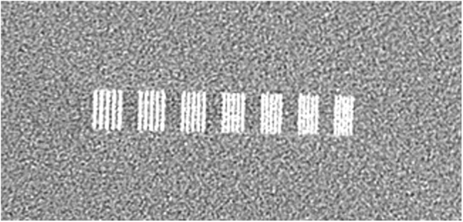
Example of a CBCT image of a line-pair phantom.

It is important to note, that this ideal system in which a line-pair would be represented by two pixels (one dark and one bright pixel) is not reality. As illustrated in Figure 3, in a real-world pixel-based system, a sharp edge is instead distributed over different neighbouring pixels. This is one effect that accounts for the entire resolution of the imaging system.

Figure 3.

An ideal imaging system (left image) using a discrete (pixel) sampling grid would display the metal edge as sharp dark–bright (e.g. black–white) discrimination between the two neighbouring pixels. However, a real-world pixel-based system (right image) distributes the edge over several neighbouring pixels and shades of grey thereby introducing blur (reduced spatial resolution) in the image. This effect is termed “edge spread function”.

Obviously, the ability to discriminate the lines against the background is also a function of the contrast between the line and background. This observation in digital radiography resulted in the development of a technical measure, the modulation transfer function (MTF).⁸ It represents the fundamental metric for the objective measurement of spatial resolution in X-ray-based tomographic modalities.⁹ Thus, it provides a more accurate measure of spatial resolution than that of simple visual assessment and has also been suggested for application in maxillofacial and dental CBCT, for example, in the new German quality assurance standard.¹⁰ Commonly, the spatial frequency at 10% contrast (modulation) is presented as the limiting frequency of a system¹¹ because observers can barely differentiate contrast <10%. To compare MTF with visual assessment, commonly the cycles per millimetre are translated into line-pairs per millimetre. This is formally not completely correct; however, one can think of a black–white sequence (line-pair) as a “cycle” (sinusoidal signal) and thus the equivalent of the two units of measurements is legitimate.

Resolution of the two-dimensional detector

Regarding spatial resolution of CBCT images, the physical resolution of the two-dimensional detector used for acquisition of the multiple projection radiographs and the resulting resolution in the 3D volume reconstructed with different algorithms must be clearly discriminated. Today, the projections acquired by a CBCT machine are commonly acquired by flat panel detectors. In the early days of CBCT, the devices generally used image intensifiers, which, among other shortcomings, provided a smaller dynamic range and also lower spatial resolution than that of today's flat panel detectors.¹² Generally, the projection images have a higher actual resolution than that of the reconstructed volumes. The signal acquired by flat panel detectors is pre-processed and, subsequently, additionally processed by pixel binning and/or noise reduction.¹³ As digital images are always sampled in a discrete fashion caused by the segmentation of the image by means of small detector elements (pixels), there is always some undersampling in digital images.¹⁴ It is well known that the discrete sampling nature of digital detectors yields sampling (aliasing) artefacts in the MTF and may also result in a “false increase” in the MTF that does not correspond to a truly enhanced spatial resolution.¹⁵ Several methods have been described for the accurate calculation of sensor resolution via pre-sampled MTF.¹⁶ The MTF of the detector can be obtained by square-shaped stripe patterns (Figure 1) on the basis of noise response¹⁷ or the Fourier transform of a slanted edge or slit image¹⁸ via its line spread function (LSF). By using the Fourier transform of the LSF, the MTF can be computed. For digital imaging systems, a characteristic difficulty arises because of the sampling grid (pixel-grid) implemented in the detectors. Thus, the detector response to a signal pattern does not depend only on the imaging properties of the detector itself. The signal pattern and its location relative to the sampling grid (Figure 4) of the detector also affect the quality of the resulting image and thus the MTF.¹⁹ Therefore, the derived MTF is influenced by two distinct components and can be considered a two-step process consisting first of the transfer of the signal, described by the pre-sampled MTF, and second of the stage of sampling (post-sampled MTF).^16,20

Figure 4.

Different orientations of an object (the dark frame) relative to the pixel sampling grid of a two-dimensional image receptor (left vs right image) produces different sampling patterns, that is, the edges are represented in different patterns of dark vs bright pixels. Considering the additional blurring effect illustrated in Figure 3, it is obvious, that this effect also influences the measured modulation transfer function of the system.

Spatial resolution in the three-dimensional reconstruction

There are several steps during image acquisition, reconstruction and display of volumetric X-ray data sets. During that process, the data are subjected to discrete sampling measures. First, the detector samples the X-ray profile emerging from the patient at a pre-determined pixel pitch. Then, a discrete number of views (projections) are used, and the data are back projected by the reconstruction algorithm into a matrix of discrete pitch (voxels). In addition, the reconstructed data may be scaled to a displayed matrix to fit the display screen. The interpolation used here also has many implications with regard to the MTF.²¹ From the Nyquist²² theorem [Equation (1)] we know that reproduction of a continuous signal requires sampling of the signal at twice the frequency of the highest frequency component contained in the signal. In other words, a fine structure of 100 μm has to be sampled by pixels of ≤50 μm to be correctly reproduced. This fact alone clearly shows that pixel/voxel size does not equal spatial resolution, as often mistakenly assumed.^4–6 It is evident that voxel size is only a bad predictor of spatial resolution.²³

The underlying reconstruction principle of CT or CBCT volumes itself is termed back projection. Most implementations employ variations of the Feldkamp–Davis–Kress (FDK) algorithm⁷ for 3D filtered back projection. Other implementations ensure iterative reconstruction techniques and low-dose protocols.²⁴ It is generally accepted that reconstructions from circular orbits are insufficient for accurate reconstructions of the volume,^25,26 which is mathematically proven by violation of the Tuy condition,²⁷ which requires that every plane intersecting the object under study must intersect the focal trajectory.²⁷ The Feldkamp et al⁷ algorithm itself only approximates the line integrals of the basic principles of the Radon transform.²⁸ The Feldkamp algorithm applies a simple approximate weight to the projection values instead of using the actual computed distances that the measured rays could have travelled from source to detector. As mentioned above, the reconstruction quality degrades with increasing cone angles.⁷ All these factors in the measurement and reconstruction process introduce artefacts into the cone beam datasets.^12,29,30

The technique to determine the MTFs for CT or CBCT scanners resembles the technique used for X-ray detectors. Initially, a measurement must be performed to obtain either the point spread function or the LSF. The usual procedure is to interpolate grey levels between the measured points in slice images reconstructed by edge phantoms (using metallic spheres or tungsten wire) and to determine the Fourier transforms numerically to obtain the MTF of the system under evaluation. Usually, this must be performed multiple times to evaluate various reconstruction kernels and scan modalities resulting in a time consuming and mostly tedious process.³¹ Currently, the typical approach for MTF assessment is to acquire an image of a small diameter metal wire positioned parallel to the long axis of the scanner.^31–35 The point spread function produced in this manner is integrated over one of the matrix directions. Equal measures are used to calculate the LSF of an edge. The Fourier transformation of the point spread function or LSF and subsequent normalization procedures are then applied to compute the MTF data of the system under evaluation.³⁶

Influence of patient motion

A factor that is often neglected during the assessment of spatial resolution for dental CBCT is the long acquisition time that is commonly several seconds (>10 s). During this time, a living patient will very likely undergo slight movements, even when seated and on a chin rest. Unfortunately, to provide a smaller voxel size, some CBCT manufacturers use a considerably longer scan time (and higher exposure) to obtain more projections for reconstruction. It seems very likely that longer scan times increase the chances for (unwanted) patient movement. Some authors have investigated the issue of patient movement using different approaches.^37,38 Strongly supporting the movement assumption above, a study regarding the optical imaging method using young and healthy volunteers has demonstrated that the heart beat alone induces a slight but relevant movement of the patient's head. Measured at the volunteer's teeth, amplitudes of approximately 80 microns per heartbeat were observed.³⁹ As the volunteers had been seated and placed with their chin on a chin rest, the position very closely resembles a patient seated in a CBCT device. Why does patient movement then influence spatial resolution? The reason is based on the assumptions required for the back projection (3D reconstruction) process. As a fundamental prerequisite for this process, the imaging geometry for each and every projection used for the process has to be accurately known. The imaging geometry is defined as a spatial relationship between the three components consisting of the focal spot, object under study and imaging plane. If a patient moves during the scan by more than the voxel size, then from the projections acquired after the movement, grey values from neighbouring structures instead of the correct structure are back projected into the volume. This results in motion blur, that is, a reduced spatial resolution,^40,41 which is a well-known fact in CT imaging. Thus far, only a few authors have stated this negative effect for maxillofacial CBCT.^37,38 From de Kinkelder's³⁹ data and the above reasoning, one can conclude that heart beat alone induces reduced spatial resolution when compared with a non-living, steady object. Based on pure logic, it is clear that longer image acquisition times yield more patient movement. Many of the studies investigating spatial resolution in CBCT are experimental and based on phantoms; therefore, this important resolution-deteriorating factor is not being considered. We are not aware of any study involving real patients that has investigated the resulting spatial resolution. Hence, we should term technically measured spatial resolution in phantoms as “nominal spatial resolution” to clearly distinguish it from the actual (reduced) spatial resolution available in living patients. As a consequence of the above explained factors, it is extremely likely that patient CBCTs will not reach the maximum spatial resolution that the CBCT device could offer. This should be taken into account when deriving clinical consequences based on measurements of structures approaching the submillimetre scale.

Review of literature

Although a systematic review was out of the scope of this work, a thorough search in PubMed using the search terms (combined with “and”) “Cone Beam CT”, “dental”, “maxillofacial” and “spatial resolution” was carried out. The entries provided by PubMed were subsequently analysed based on the abstracts, and the articles that provided information on spatial resolution of CBCT machines (line-pairs per millimetre or MTF or both measures) used for dental or maxillofacial applications were selected and evaluated. This resulted in a final number of ten^9,42–50 articles that are summarized in Table 1. It should be noted that the values reported in studies by Watanabe et al^49,50 are identical because the second report⁵⁰ compares the values presented under a technical aspect in the first article⁴⁹ with those obtained from medical CT. Out of the ten articles,^9,42–50 nine measured line-pair resolution^9,43–50 in one way or another and only six^{9,42–45,49,50} assessed MTF. Altogether, the articles present quite similar results (Table 1). Spatial resolution assessed visually and expressed by discriminated line-pairs per millimetre ranged between 0.6 lp mm⁻¹ and a maximum of 2.8 lp mm⁻¹. From a combined analysis of the data, a median value of approximately 1.7 lp mm⁻¹ [or (cycles per millimetre)] is evident (Figure 5).

Table 1.

Spatial resolution of current CBCT scanners as published in recent literature

Publication	Type of phantom	Visual resolution (lp mm−1)		MTF at 10% modulation (cycles per millimetre)		Voxel size (range in millimetre)		CBCT device(s)
		Min	Max	Min	Max	Min	Max
Suomalainen et al42	Teflon® edge vs Perspex® background	na	na	0.10	0.80	0.120	0.360	3D Accuitomo
								PromaxH 3D scanner
								Scanora® 3D scanner
Xu et al43	Wire phantom	1.20	1.6	1.80	2.30	0.200	0.500	CS 9300
Ozaki et al44	Thin tungsten wire	1.70	2.8	1.80	2.60	0.080	0.160	3D Accuitomo FineCube v. 12
Bamba et al45	SEDENTEXCT, thin stainless steel vs air	1.00	2.8	0.60	1.25	0.080	0.125	CS 9300
								3D Accuitomo 80
								Veraviewepocs
Ballrick et al46	Line-pair phantom [C phantom (Phantom Laboratory, Salem, NY)]	0.60	0.8	na	na	0.200	0.400	i-CAT model 9140-0035-000C
Knörgen et al47	Edge PMMA vs air	0.70	1.7	na	na	0.125	0.250	3D Accuitomo 170
Pauwels et al48	SEDENTEXCT, line-pair insert (aluminium vs polymer)	na	<3.0	na	na	0.076	0.400	3D Accuitomo 170
								3D Accuitomo (image intensifier)
								Veraviewepocs
								Galileos Comfort
								i-CAT Next Generation
								CS 9000 3D
								CS 9500
								NewTom VGi
								Pax-Uni3D
								Picasso Trio
								ProMax® 3D
								Scanora 3D scanner
								SkyView®
Steiding et al9	Edge aluminium sphere vs foam	0.83	1.0	0.88	0.89	0.300	0.300	i-CAT Next Generation
Watanabe et al49	0.100-mm tungsten wire; MTF, 0.100-mm tungsten wire; visual, aluminium vs epoxy resin	1.90	2.1	1.75	2.64	0.125	0.125	3D Accuitomo (image intensifier)
Watanabe et al50	MTF, 0.100-mm tungsten wire; visual, aluminium vs epoxy resin	1.90	2.1	1.89	2.65	0.125	0.125	3D Accuitomo (image intensifier)

max, maximum; min, minimum; MTF, modulation transfer function; na, not available; PMMA, polymethylmethacrylate.

3D Accuitomo, Veraviewepocs and FineCube v. 12 obtained from J. Morita MFG Corp., Kyoto, Japan; PromaxH 3D scanner obtained from Planmeca Oy, Helsinki, Finland; Scanora^® 3D scanner obtained from Soredex, Tuusula, Finland; CS 9300, CS 9000 3D and CS 9500 obtained from Carestream Health, Rochester, NY; i-CAT model 9140-0035-000C obtained from Imaging Sciences International, Hatfield, PA; Galileos Comfort obtained from Sirona Dental Systems, Bensheim, Germany; NewTom VGi obtained from Quantitative Radiology (QR Srl), Verona, Italy; Pax-Uni3D and Picasso Trio obtained from Value Added Technologies (VATECH), Yongin, South Korea; SkyView obtained from Cefla Dental Group, Imola, Italy.

Figure 5.

Meta-analysis of the articles in Table 1, visually discernable line-pairs (lp) (left boxplot) vs modulation transfer function (MTF) data (right box).

Figure 5 indicates a larger variation between the values for the MTF (range, 0.5–2.3 cycles per millimetre; median, 2.1 cycles per millimetre) data when compared with the visual line-pair assessment. However, the data presented in Table 1 and Figure 5 also indicate a fair agreement between visually discernible line-pairs per millimetre and the frequency at 10% modulation (Table 1, Figure 5). Pauwels et al⁴⁸ from the SEDENTEXCT-project observed a general limit of <3 lp mm⁻¹ in their assessment of 13 different CBCT devices and scan protocols. With respect to MTF, the objective technical measure, the reports ranged from 0.1 cycle per millimetre⁴² to a maximum of 2.65 cycles per millimetre.⁵⁰ While the higher resolutions reported seem to reflect a “best possible” scenario, it is interesting that the authors attribute the lowest reported values⁴² to a realistic scattering and attenuation environment applied in their experiments. The authors had used a head-sized phantom intentionally designed to resemble the absorption conditions of the human head.⁴² For the visual line-pair assessment, a mean (± standard deviation) of 1.54 (±0.57) lp mm⁻¹ was computed (median, 1.65 lp mm⁻¹). The MTF at 10% modulation revealed a mean of 1.60 (±0.83) cycles per millimetre with a median value of 2.05 lp mm⁻¹ (Table 1).

For illustration purposes, we computed an exemplary MTF curve from our own device (3DExam, i-CAT^® Next Generation; Imaging Sciences International, Hatfield, PA) for a pre-selected voxel size of 0.3 mm that is shown in Figure 6. This smoothened graph reveals an approximate spatial resolution of 1.4 cycles per millimetre at 10% modulation, which conforms to the data reported in the literature.

Figure 6.

Exemplary (smoothed) modulation transfer function plot for the 3DExam device (i-CAT^® Next Generation; Imaging Sciences International, Hatfield, PA) for a voxel size of 0.3 mm.

As a consequence, a general article addressing the CBCT performance issues suggested a spatial resolution of ≥1 lp mm⁻¹ in high-resolution mode⁵¹ to qualify as dental CBCT.

Discussion

Spatial resolution refers to the ability of an imaging system to depict fine details contained in the object under study. It represents one of many essential image properties describing the quality of an imaging system. As an “objective” measure, the MTF represents the fundamental metric for the objective measurement of spatial resolution in X-ray-based tomographic modalities.⁹ Interestingly, in the studies on spatial resolution in CBCT,^9,42–50 we found a larger variance between the MTF values when comparing them to the visually assessed line-pair per millimetre. Neitzel et al⁵² have demonstrated that an MTF assessment at the edge is very dependent on the physical absorption parameters and the amount of noise at that edge. Certainly, this also holds true for other assessment methods, such as thin wires or edges between other materials, as applied in some of the articles assessed in this review.^42,47 As explicitly stated by Suomalainen et al,⁴² the authors attribute their low MTF values to the head phantom resembling a “natural” scatter environment.

Owing to inevitable errors in the imaging chain and the requirements from the fundamental Nyquist theorem, actual available spatial resolution will always be considerably less than the physical voxel size. This can be clearly seen from the MTF plots,^9,49 in which the modulation (the contrast) at Nyquist frequency is around zero. Thus, as also stated by other authors, a voxel is only a very crude predictor of available spatial resolution.²³ Owing to the mechanical construction of CBCT machines, which require a relatively slow trajectory of the source–image detector unit around the patient's head, a slight patient movement seems almost inevitable. Given the small voxel sizes applied in the machines, a slight movement of more than voxel size will induce errors in the reconstruction. As a result, motion blur, which is very well known in medical CT,⁴⁰ will occur thereby further negatively affecting the available spatial resolution.

The analysis of the articles used for this review indicates a theoretically available spatial resolution in a “best possible” experimental scenario of <3 lp mm⁻¹ with a median value of approximately 2 lp mm⁻¹. A real-world CBCT scan of a small volume will always suffer from the scatter of tissues around the small field of view. As explained above, this will reduce the available resolution.⁴² Unavoidable slight movement of the living patient will have the same effect. Considering the data from this review and these effects in real-world CBCT images, one could estimate a truly available spatial resolution of slightly >1 lp mm⁻¹. This would translate to a realistic detail size of 500 microns that could be visualized in a high-quality CBCT of a “visually steady” (i.e. only moving owing to heart beat) patient. These error margins should be kept in mind whenever planning is based on CBCT images that require assessment/estimation at the submillimetre dimension. It seems quite obvious that the latter is hard to achieve.

It is important to note here that spatial resolution of intraoral radiography is around one order of magnitude higher, that is, around >10 lp mm⁻¹ at 10% contrast.⁵³ In other words, a truly high-resolution image is only available in two-dimensional radiographic images. Unfortunately, there is no technical solution at this time to improve this parameter significantly in 3D because it would require even longer scan times and redundant data sampling as performed in micro-CT for non-living objects. However, apart from the obvious dose increase, a longer acquisition time would result in even more patient movement thereby reducing effective spatial resolution.

In conclusion, our review of measured spatial resolution in an experimental set-up reveals a range of approximately 1–2 lp mm⁻¹. These data have been acquired in experimental situations using phantoms and represent what we term “nominal spatial resolution”. Owing to the Nyquist theorem and other image degrading factors, the latter is considerably lower than predicted based on voxel size. Patient movement in magnitudes exceeding voxel size will further reduce available spatial resolution. As a clinical consequence, it is important to not overestimate spatial resolution in CBCT volumes. The minimum value of approximately 1 lp mm⁻¹ that was suggested in the study by Horner et al⁵¹ to qualify as dental CBCT yields a resulting visibility of details of only 500 microns, i.e. 0.5 mm. Hence, during a clinical application, one cannot expect higher accuracy than in the range of half a millimetre at best. If in doubt, the user should avoid submillimetre accuracy and preferably add some margin of error to his/her planning.

References

- 1.Mozzo P, Procacci C, Tacconi A, Martini PT, Andreis IA. A new volumetric CT machine for dental imaging based on the cone-beam technique: preliminary results. Eur Radiol 1998; 8: 1558–64. [DOI] [PubMed] [Google Scholar]
- 2.Ralph WJ, Jefferies JR. The minimal width of the periodontal space. J Oral Rehabil 1984; 11: 415–18. [DOI] [PubMed] [Google Scholar]
- 3.Nemtoi A, Czink C, Haba D, Gahleitner A. Cone beam CT: a current overview of devices. Dentomaxillofac Radiol 2013; 42: 20120443. doi: 10.1259/dmfr.20120443 [DOI] [PMC free article] [PubMed] [Google Scholar]
- 4.Kamburoğlu K, Kursun S. A comparison of the diagnostic accuracy of CBCT images of different voxel resolutions used to detect simulated small internal resorption cavities. Int Endod J 2010; 43: 798–807. doi: 10.1111/j.1365-2591.2010.01749.x. [DOI] [PubMed] [Google Scholar]
- 5.Tyndall DA, Kohltfarber H. Application of cone beam volumetric tomography in endodontics. Aust Dent J 2012; 1: 72–81. [DOI] [PubMed] [Google Scholar]
- 6.Michetti J, Maret D, Mallet JP, Diemer F. Validation of cone beam computed tomography as a tool to explore root canal anatomy. J Endod 2010; 36: 1187–90. [DOI] [PubMed] [Google Scholar]
- 7.Feldkamp LA, Davis LC, Kress JW. Practical cone-beam algorithm. J Opt Soc Am 1984; 1: 612–19. [Google Scholar]
- 8.Fujita H, Tsai DY, Itoh T, Doi K, Morishita J, Ueda K, et al. A simple method for determining the modulation transfer function in digital radiography. IEEE Trans Med Imaging 1992; 11: 34–9. [DOI] [PubMed] [Google Scholar]
- 9.Steiding C, Kolditz D, Kalender WA. A quality assurance framework for the fully automated and objective evaluation of image quality in cone-beam computed tomography. Med Phys 2014; 41: 031901. doi: 10.1118/1.4863507 [DOI] [PubMed] [Google Scholar]
- 10.Deutsches Institut für Normung DIN. Sicherung der Bildqualität in röntgendiagnostischen Betrieben—Teil 161: Abnahmeprüfung nach RöV an zahnmedizinischen Röntgeneinrichtungen zur digitalen Volumentomographie; Beuth Verlag GmbH: Berlin Januar 2013 (6868–161).
- 11.Allisy-Roberts P, Williams J. Farr's physics for medical imaging. 2nd edn. St Louis, MO: Saunders; 2007. [Google Scholar]
- 12.Kalender WA, Kyriakou Y. Flat-detector computed tomography (FD-CT). Eur Radiol 2007; 17: 2767–79. [DOI] [PMC free article] [PubMed] [Google Scholar]
- 13.Brüllmann DD, d'Hoedt B. The modulation transfer function and signal-to-noise ratio of different digital filters: a technical approach. Dentomaxillofac Radiol 2011; 40: 222–9. [DOI] [PMC free article] [PubMed] [Google Scholar]
- 14.Dobbins JT, 3rd. Effects of undersampling on the proper interpretation of modulation transfer function, noise power spectra, and noise equivalent quanta of digital imaging systems. Med Phys 1995; 22: 171–81. [DOI] [PubMed] [Google Scholar]
- 15.Giger ML, Doi K. Investigation of basic imaging properties in digital radiography. I. Modulation transfer function. Med Phys 1984; 11: 287–95. [DOI] [PubMed] [Google Scholar]
- 16.Buhr E, Günther-Kohfahl S, Neitzel U. Accuracy of a simple method for deriving the presampled modulation transfer function of a digital radiographic system from an edge image. Med Phys 2003; 30: 2323–31. [DOI] [PubMed] [Google Scholar]
- 17.Kuhls-Gilcrist A, Jain A, Bednarek DR, Hoffmann KR, Rudin S. Accurate MTF measurement in digital radiography using noise response. Med Phys 2010; 37: 724–35. [DOI] [PMC free article] [PubMed] [Google Scholar]
- 18.Friedman SN, Cunningham IA. Normalization of the modulation transfer function: the open-field approach. Med Phys 2008; 35: 4443–9. [DOI] [PubMed] [Google Scholar]
- 19.Hadar O, Dogariu A, Boreman GD. Angular dependence of sampling modulation transfer function. Appl Opt 1997; 36: 7210–16. [DOI] [PubMed] [Google Scholar]
- 20.Pratt WK. Digital image processing. New York, NY: John Wiley & Sons, Inc.; 1991. [Google Scholar]
- 21.Boone JM. Determination of the presampled MTF in computed tomography. Med Phys 2001; 28: 356–60. [DOI] [PubMed] [Google Scholar]
- 22.Nyquist H. Certain topics in telegraph transmission theory. Trans Am Inst Elec Eng 1928; 47: 617–44. [Google Scholar]
- 23.Pauwels R, Stamatakis H, Manousaridis G, Walker A, Michielsen K, Bosmans H, et al. Development and applicability of a quality control phantom for dental cone-beam CT. J Appl Clin Med Phys 2011; 12: 3478. doi: 10.1120/jacmp.v12i4.3478 [DOI] [PMC free article] [PubMed] [Google Scholar]
- 24.Hara AK, Paden RG, Silva AC, Kujak JL, Lawder HJ, Pavlicek W. Iterative reconstruction technique for reducing body radiation dose at CT: feasibility study. AJR Am J Roentgenol 2009; 193: 764–71. doi: 10.2214/AJR.09.2397 [DOI] [PubMed] [Google Scholar]
- 25.Mueller K. Fast and accurate three-dimensional reconstruction from cone-beam projection data using algebraic methods. Columbus, OH: The Ohio State University; 1998. [Google Scholar]
- 26.Yu L, Pan X, Peliizari CA. Image reconstruction with a shift-variant filtration in circular cone-beam CT. Int J Imaging Syst Technol 2005; 14: 213–21. doi: 10.1002/ima.20026 [DOI] [Google Scholar]
- 27.Tuy HK, Siam J. An inversion formula for cone-beam reconstruction. Appl Math 1983; 43: 546–52. [Google Scholar]
- 28.Schulze R, Heil U, Gross D, Bruellmann D, Dranischnikow E, Schwanecke U, et al. Artefacts in CBCT: a review. Dentomaxillofac Radiol 2011; 40: 265–73. doi: 10.1259/dmfr/30642039 [DOI] [PMC free article] [PubMed] [Google Scholar]
- 29.Sharp GC, Kanasamy N, Singh H, Folkert M. GPU-based streaming architectures for fast cone-beam CT image reconstruction and demons deformable registration. Phys Med Biol 2007; 52: 5771–83. [DOI] [PubMed] [Google Scholar]
- 30.Zhang Y, Zhang L, Zhu XR, Lee AK, Chambers M, Dong L. Reducing metal artifacts in cone-beam CT images by preprocessing projection data. Int J Radiat Oncol Biol Phys 2007; 67: 924–32. [DOI] [PubMed] [Google Scholar]
- 31.Nickoloff EL, Riley R. A simplified approach for modulation transfer function determinations in computed tomography. Med Phys 1985; 12: 437–42. [DOI] [PubMed] [Google Scholar]
- 32.Droege RT, Morin RL. A simplified approach for modulation transfer function determinations in computed tomography. Med Phys 1982; 9: 758–60. [DOI] [PubMed] [Google Scholar]
- 33.Bischof CJ, Ehrhardt JC. Modulation transfer function of the EMI CT head scanner. Med Phys 1977; 4: 163–7. [DOI] [PubMed] [Google Scholar]
- 34.Judy PF. The line spread function and modulation transfer function of a computed tomographic scanner. Med Phys 1976; 3: 233–6. [DOI] [PubMed] [Google Scholar]
- 35.Durand EP, Rüegsegger P. High-contrast resolution of CT images for bone structure analysis. Med Phys 1992; 19: 569–73. [DOI] [PubMed] [Google Scholar]
- 36.Dainty JC, Shaw R, eds. Image science: principles, analysis and evaluation of photographic-type imaging processes. London, UK: Academic Press Inc.; 1974. [Google Scholar]
- 37.Hanzelka T, Dusek J, Ocasek F, Kucera J, Sedy J, Benes J, et al. Movement of the patient and the cone beam computed tomography scanner: objectives and possible solutions. Oral Surg Oral Med Oral Pathol Oral Radiol 2013; 116: 769–73. doi: 10.1016/j.oooo.2013.08.010 [DOI] [PubMed] [Google Scholar]
- 38.Spin-Neto R, Mudrak J, Matzen LH, Christensen J, Gotfredsen E, Wenzel A. Cone beam CT image artefacts related to head motion simulated by a robot skull: visual characteristics and impact on image quality. Dentomaxillofac Radiol 2013; 42: 32310645. doi: 10.1259/dmfr/32310645 [DOI] [PMC free article] [PubMed] [Google Scholar]
- 39.de Kinkelder R, Kalkman J, Faber DJ, Schraa O, Kok PH, Verbraak FD, et al. Heartbeat-induced axial motion artifacts in optical coherence tomography measurements of the retina. Invest Ophthalmol Vis Sci 2011; 52: 3908–13. doi: 10.1167/iovs.10-6738 [DOI] [PubMed] [Google Scholar]
- 40.Bergner F, Berkus T, Oelhafen M, Kunz P, Pa T, Grimmer R, et al. An investigation of 4D cone-beam CT algorithms for slowly rotating scanners. Med Phys 2010; 37: 5044–53. [DOI] [PubMed] [Google Scholar]
- 41.Zhang K, Li M, Dai J, Wang S. Image quality of cone beam CT on respiratory motion. Nucl Sci Tech 2011; 22: 111–17. [Google Scholar]
- 42.Suomalainen A, Kiljunen T, Käser Y, Peltola J, Kortesniemi M. Dosimetry and image quality of four dental cone beam computed tomography scanners compared with multislice computed tomography scanners. Dentomaxillofac Radiol 2009; 38: 367–78. doi: 10.1259/dmfr/15779208 [DOI] [PubMed] [Google Scholar]
- 43.Xu J, Reh DD, Carey JP, Mahesh M, Siewerdsen JH. Technical assessment of a cone-beam CT scanner for otolaryngology imaging: image quality, dose, and technique protocols. Med Phys 2012; 39: 4932–42. doi: 10.1118/1.4736805 [DOI] [PubMed] [Google Scholar]
- 44.Ozaki Y, Watanabe H, Nomura Y, Honda E, Sumi Y, Kurabayashi T. Location dependency of the spatial resolution of cone beam computed tomography for dental use. Oral Surg Oral Med Oral Pathol Oral Radiol 2013; 116: 648–55. doi: 10.1016/j.oooo.2013.07.009 [DOI] [PubMed] [Google Scholar]
- 45.Bamba J, Araki K, Endo A, Okano T. Image quality assessment of three cone beam CT machines using the SEDENTEXCT CT phantom. Dentomaxillofac Radiol 2013; 42: 20120445. doi: 10.1259/dmfr.20120445 [DOI] [PMC free article] [PubMed] [Google Scholar]
- 46.Ballrick JW, Palomo JM, Ruch E, Amberman BD, Hans MG. Image distortion and spatial resolution of a commercially available cone-beam computed tomography machine. Am J Orthod Dentofacial Orthop 2008; 134: 573–82. doi: 10.1016/j.ajodo.2007.11.025 [DOI] [PubMed] [Google Scholar]
- 47.Knörgen M, Brandt S, Kösling S. Comparison of quality on digital X-ray devices with 3D-capability for ENT-clinical objectives in imaging of temporal bone and paranasal sinuses. [In German.] Rofo 2012; 184: 1153–60. doi: 10.1055/s-0032-1325343 [DOI] [PubMed] [Google Scholar]
- 48.Pauwels R, Beinsberger J, Stamatakis H, Tsiklakis K, Walker A, Bosmans H, et al. Comparison of spatial and contrast resolution for cone-beam computed tomography scanners. Oral Surg Oral Med Oral Pathol Oral Radiol 2012; 114: 127–35. [DOI] [PubMed] [Google Scholar]
- 49.Watanabe H, Honda E, Kurabayashi T. Modulation transfer function evaluation of cone beam computed tomography for dental use with the oversampling method. Dentomaxillofac Radiol 2010; 39: 28–32. doi: 10.1259/dmfr/27069629 [DOI] [PMC free article] [PubMed] [Google Scholar]
- 50.Watanabe H, Honda E, Tetsumura A, Kurabayashi T. Modulation transfer function evaluation of cone beam computed tomography for dental use with the oversampling method. Eur J Radiol 2011; 39: 28–32. doi: 10.1259/dmfr/27069629 [DOI] [PMC free article] [PubMed] [Google Scholar]
- 51.Horner K, Jacobs R, Schulze R. Dental CBCT equipment and performance issues. Radiat Prot Dosimetry 2013; 153: 212–18. doi: 10.1093/rpd/ncs289 [DOI] [PubMed] [Google Scholar]
- 52.Neitzel U, Buhr E, Hilgers G, Granfors PR. Determination of the modulation transfer function using the edge method: influence of scattered radiation. Med Phys 2004; 31: 3485–91. [DOI] [PubMed] [Google Scholar]
- 53.Brüllmann DD, Kempkes B, d'Hoedt B, Schulze R. Contrast curves of five different intraoral X-ray sensors: a technical note. Oral Surg Oral Med Oral Pathol Oral Radiol 2013: 115: e55–61. doi: 10.1016/j.oooo.2013.03.007 [DOI] [PubMed] [Google Scholar]